


Abstract
We present a detailed high spectral resolution (R ∼ 40 000) study of five high-z damped Lyman α systems (DLAs) and one sub- DLA detected along four QSO sightlines. Four of these DLAs are very metal poor with [Fe/H] ≤ −2. One of them, at zabs = 4.202 87 towards J0953−0504, is the most metal-poor DLA at z > 4 known till date. This system shows no enhancement of C over Fe and O, and standard Population II star yields can explain its relative abundance pattern. The DLA at zabs = 2.340 06 towards J0035−0918 has been claimed to be the most carbon-enhanced metal-poor DLA. However, we show that thermal broadening is dominant in this system and, when this effect is taken into account, the measured carbon enhancement ([C/Fe] = 0.45 ± 0.19) becomes ∼10 times less than what was reported previously. The gas temperature in this DLA is estimated to be in the range of 5000–8000 K, consistent with a warm neutral medium phase. From photoionization modelling of two of the DLAs showing C ii* absorption, we find that the metagalactic background radiation alone is not sufficient to explain the observed C ii* cooling rate, and local heating sources, probably produced by in situ star formation, are needed. Cosmic ray heating is found to contribute ≳60 per cent to the total heating in these systems. Using a sample of metal-poor DLAs with C ii* measurements, we conclude that the cosmic ray ionization rate is equal to or greater than that seen in the Milky Way in ∼33 per cent of the systems with C ii* detections.
1 INTRODUCTION
Understanding the formation and evolution of the first generation of stars would help in fathoming the initial chemical conditions and evolution of the Universe (Bromm & Larson 2004). In addition, it is believed that the radiation from such Population III stars may have played an important role in the reionization of the Universe. These massive stars emit 1047–10|$^{48} \,\rm{H\,{\small I}}$| and |$\rm{He\,{\small I}}$| ionizing photons per second per solar mass of formed stars, where the lower value holds for stars of ∼20 M⊙ and the upper value applies to stars with ≳100 M⊙ (see Tumlinson & Shull 2000; Bromm, Kudritzki & Loeb 2001). However, their lifetimes are short (∼3 × 10⁶ yr), and hence, it would be very difficult to observe them directly. Nevertheless, we can try to infer signatures of Population III stars in the most metal-poor environments detected in nature. Recently, there have also been indications of Population III star formation in the Universe, even as late as z ∼ 3, possibly due to inefficient transport of heavy elements and/or poor mixing that leaves pockets of pristine gas (Jimenez & Haiman 2006; Tornatore, Ferrara & Schneider 2007; Inoue et al. 2011; Cassata et al. 2013).
The metal-poor stars in the halo of the Milky Way are being studied in an effort to understand the chemical composition and hence the nature of star formation at very early epochs (see Akerman et al. 2004; Cayrel et al. 2004; Beers & Christlieb 2005; Frebel 2010). Such studies can also be used to infer the chemical evolution in the Universe, if most galaxies follow the chemical history of the Milky Way. However, the measurement of abundances in stellar atmospheres is hampered by having to take into account non-local thermodynamic equilibrium effects as well as three-dimensional effects in one-dimensional stellar atmosphere models (Asplund 2005). In addition, the presence of convection or accretion of material from a companion can affect the photospheric abundance measurements. Hence, these measurements may not always trace well the chemical evolution history of the Galaxy.
These issues are not present when one studies damped Lyα systems (DLAs), which are by definition, clouds of neutral gas with neutral hydrogen column density N(|$\rm{H\,{\small I}}$|) > 2 × 10|$^{20} \,\rm{H\,{\small I}}$| atoms cm−2 (see Wolfe, Gawiser & Prochaska 2005 for a review). The high N(|$\rm{H\,{\small I}}$|) self-shields the gas from the ultraviolet (UV) background radiation of quasars (QSOs) and galaxies. Due to this, abundance measurements require negligible ionization corrections, i.e. hydrogen gas in DLAs is mostly neutral and most of the heavy elements are either neutral or singly ionized (Pettini et al. 2002; Prochaska et al. 2002; Centurión et al. 2003; Ledoux, Petitjean & Srianand 2003). Even then, line saturation and presence of dust may hinder abundance measurements in DLAs. However, when the metallicity of the DLAs happens to be ≲10−2 Z⊙ (i.e. in so-called metal-poor DLAs), these issues are also mitigated (for e.g. Akerman et al. 2005), especially for the estimation of C, N and O abundances. Moreover, high-z metal-poor DLAs are believed to probe gas in or around protogalaxies, and hence contain pieces of evidence of the earliest star formation and retain signatures of the initial chemical enrichment. The relative abundances of C, N, O, Fe, etc. in low-metallicity DLAs can give insights into the type of stars (specifically the stellar initial mass function, IMF) that led to their production, and hence shed light on our understanding of galactic nucleosynthesis and chemical evolution (Petitjean, Ledoux & Srianand 2008; Pettini et al. 2008; Penprase et al. 2010; Cooke et al. 2011b). In view of this, we undertake a study of five DLAs (pre-selected as candidate low-metallicity DLAs), and their elemental abundances, and compare our results with the existing measurements of low-metallicity DLAs and stars in the Galactic halo.
There is an ongoing interest in detecting and studying the properties of metal-poor DLAs. Pettini et al. (2008) studied a sample of four metal-poor DLAs (defined as those with [Fe/H] ≤ −2.0) using high-resolution spectra (R ∼ 40 000) from Keck and Very Large Telescope (VLT). They found that the C/O ratio trend at low metallicity in high-redshift DLAs matches that of halo stars in the Galaxy (Akerman et al. 2004; Spite et al. 2005), and the ratio shows higher values that cannot be explained by nucleosynthesis models based on Population II stars. Their results also suggested that the N/O ratio at low metallicities may show a minimum value. Penprase et al. (2010) used medium-resolution spectra (R ∼ 5000) to study a sample of 35 DLAs pre-selected as metal-poor from the Sloan Digital Sky Survey (SDSS) DR5 data base. However, while medium-resolution spectra are sufficient to detect metal-poor DLAs, one needs to be cautious about employing them to measure accurate abundances in the most metal-poor systems, which typically have line widths ≲10 km s−1.
Measurements of seven new metal-poor DLAs observed with high-resolution spectrograph were reported by Cooke et al. (2011b), who have also compiled a sample of all the (22) metal-poor DLAs known in the literature. Using this sample and taking oxygen as the reference element, they have defined the typical abundance pattern of a very metal poor (VMP) DLA by determining the mean 〈X/O〉 ratio for each available element X, and then referring this mean value to the adopted solar scale. On comparing this with the yields of both Population II and III stars, it is found that, while a standard model of Population III stars (a top-heavy IMF where the stars explode as core-collapse supernovae) gives reasonable agreement with the observed abundance pattern of a typical VMP DLA, the possibility that Population II stars may account for the observed abundances cannot be discarded. To distinguish between these two nucleosynthesis models, the [C/Fe] ratio is useful, as current models of Population II stars cannot explain an enhanced [C/Fe] ratio (along with [N/Fe] ≲ 0). An enhanced [O/Fe] ratio (≳0.4) will also be an useful discriminatory tool, since enhanced [C/Fe] is likely to lead to enhanced [O/Fe]. There are only two examples of carbon enhancement in metal-poor DLAs (Cooke et al. 2011a; Cooke, Pettini & Murphy 2012), which are likely to be the outcome of nucleosynthesis in massive stars. Understanding the abundance pattern in these carbon-enhanced metal-poor (CEMP) DLAs and increasing their number is important for understanding the true metal yields from very massive stars.
In addition, since DLAs are the main reservoirs of neutral gas at high-z (Prochaska, Herbert-Fort & Wolfe 2005; Noterdaeme et al. 2009b), studying their star formation properties is important, as they could contribute significantly to the global star formation rate (SFR) density at high-z (for e.g. Wolfe et al. 2008; Rahmani et al. 2010). Detection of H2 or |$\rm{C\,{\small II}}$|* absorption in DLAs can allow us to study the physical conditions in the absorbing gas, and also in principle to infer the SFR (see Wolfe, Prochaska & Gawiser 2003a; Srianand et al. 2005). In the present sample, we have observed |$\rm{C\,{\small II}}$|* absorption associated with two of the DLAs. The |$\rm{C\,{\small II}}$|* λ1335 column density has been used to measure the [|$\rm{C\,{\small II}}$|] λ158 μm cooling rate in the neutral gas. We simulate the physical conditions in these two DLAs, and try to match the model predictions with the observations in order to infer the ambient radiation field and cosmic ray (CR) ionization rate in these DLAs. Further, we look at all the detections of |$\rm{C\,{\small II}}$|* in metal-poor DLAs reported till date and try to relate the |$\rm{C\,{\small II}}$|* absorption to the metallicity and N(|$\rm{H\,{\small I}}$|), in order to understand the physical conditions in such DLAs.
This paper is organized as follows. In Section 2, we give details of the observations and data reduction process. How the analysis of the data was carried out is explained is Section 3. Section 4 gives description of the individual absorption systems. In Section 5, we discuss the trends observed in abundance ratios of elements in metal-poor DLAs. We discuss the detection of |$\rm{C\,{\small II}}$|* in metal-poor DLAs and its implications in Section 6. Lastly, we summarize our results and present the conclusions in Section 7.
2 OBSERVATIONS AND DATA REDUCTION
The spectra of the objects studied in this project have been obtained with European Southern Observatory's (ESO) Ultraviolet and Visual Echelle Spectrograph (UVES) on the VLT [Programme ID: 086.A-0204 and 383.A-0272, PI: P. Petitjean]. For two objects, J0953−0504 and J0035−0918, we also use the Keck High Resolution Echelle Spectrometer (HIRES) spectra that are available in the online archive.1 One of the objects (J0953−0504) was selected from the sample of DLAs gathered during the H2 molecules survey (see Noterdaeme et al. 2008), by checking by eye those DLAs with reported [Fe/H] ≤ −2.0. The other systems were selected from the SDSS DR7 DLA catalogue (Noterdaeme et al. 2009a), based on the weakness/absence of strong metal absorption lines in DLAs with large neutral hydrogen column densities. The targets were chosen after checking by eye those DLAs without detectable metal lines or very weak |$\rm{C\,{\small II}}$| lines (which always remain visible in careful eye-checking). This is a justified method of selecting metal-poor DLAs for further study, since the strongest metal lines should remain undetected at the low resolution and signal-to-noise ratio (S/N) of the SDSS spectra, for the system to be a metal-poor DLA. However, the lack of detection does not guarantee low metallicity since it could be a consequence of lines with very low-velocity width (Δv ≲ 10 km s−1) being washed out by low resolution. Note that from the correlation found by Ledoux et al. (2006) we expect systems with narrow metal lines to have low metallicity. In any case, to get accurate estimate of the metallicities, we need to use the high-resolution spectra.
In Table 1, we present details of the observations. All the UVES spectra were reduced using the Common Pipeline Library data reduction pipeline using an optimal extraction method. All the spectra, after applying barycentric correction, were brought to their vacuum values using the formula given in Edlen (1966). For the co-addition, we interpolated the individual spectra and their errors to a common wavelength array, and then computed the weighted mean using the weights estimated from the error in each pixel. In the case of Keck/HIRES spectra, we use the pipeline calibrated data available in the Keck archive. The wavelength range covered, spectral resolution and average S/N for each QSO are also given in Table 1. In total, we have five DLAs and one sub-DLA along the four QSO sightlines considered here.
Details of observations.
| QSO | zem | zabs | Telescope/ | Wavelength | Resolution | S/Nb | Integration |
|---|---|---|---|---|---|---|---|
| instrument | range (Å)a | (km s−1) | time (s) | ||||
| J003501.88−091817.6 | 2.413 | 2.340 06 | VLT/UVES | 3760–9460 | 6.0 | 13 | 2 × 3000 |
| KECK/HIRES | 3500–6000 | 7.0 | 16 | 6 × 2700 | |||
| J023408.97−075107.6 | 2.540 | 2.318 15 | VLT/UVES | 3760–9460 | 6.0 | 19 | 5 × 3000 |
| J095355.69−050418.5 | 4.369 | 4.202 87 | VLT/UVES | 4780–6810 | 6.0 | 28 | 4 × 7740 |
| KECK/HIRES | 6030–8390 | 7.0 | 12 | 1 × 7200, 1 × 9000 | |||
| J100428.43+001825.6 | 3.045 | 2.539 70 | VLT/UVES | 4160–6210 | 6.0 | 26 | 6 × 3004 |
| 2.685 37 | |||||||
| 2.745 75 |
aWith some wavelength gaps.
bS/N per pixel measured at ∼5000 Å (or ∼7000 Å for J0953-0504 HIRES spectrum).
3 DATA ANALYSIS
The metal absorption lines of the DLAs are modelled by Voigt profile using the vpfit software package (version 9.5).2vpfit employs χ2 minimization to simultaneously fit Voigt profiles to a set of absorption lines, governed by three free parameters: (1) absorption redshift (zabs); (2) Doppler parameter (b in km s−1); and (3) column density (N). The number of components to fit was initially decided by the profiles of the unsaturated metal transitions in the system. We then tried to obtain a good fit by maintaining the |$\chi ^{2}_{\rm red}$| close to 1.0, and the errors on the fitted parameters reasonable. We assumed that all the neutral and first ions (e.g. |$\rm{C\,{\small II}}$|, |$\rm{N\,{\small I}}$|, |$\rm{O\,{\small I}}$|, |$\rm{Si\,{\small II}}$|, |$\rm{S\,{\small II}}$|, |$\rm{Fe\,{\small II}}$|) are kinematically associated with the same gas cloud. Hence, the redshift and b parameter for each absorption component are tied to be the same for each of the ions, i.e. basically considering only the turbulent component of the broadening. However, in cases where we observe that the metal lines are very narrow, we leave both the turbulent velocity bturb and the temperature T as free variables during the fitting procedure, to check if there is any significant contribution from the thermal broadening. vpfit calculates the errors on each of the fitted parameters, and the errors in ion column densities quoted here are those provided by vpfit. The neutral hydrogen column densities of the DLAs were determined by fitting the damping wings of the Lyα line (which are very sensitive to N(|$\rm{H\,{\small I}}$|)). The error in N(|$\rm{H\,{\small I}}$|) measurement was estimated by trying different continua near the Lyα line profile. For a given continuum, the statistical fitting error from vpfit is small (∼0.03 dex) and the error is dominated by continuum placement uncertainties.
The abundances of elements were deduced by assuming that each element resides in a single dominant ionization stage in the neutral gas. This assumption is valid in DLAs as they are self-shielded from metagalactic ionizing radiation as well as local radiation fields (for E > 13.6 eV), due to the high N(|$\rm{H\,{\small I}}$|). While absorption of metals are seen in several components, we measure |$\rm{H\,{\small I}}$| as one component. Hence, abundance of an element X is determined by taking the ratio of the total column density (sum of column densities in all detected individual components) of its dominant ion to that of |$\rm{H\,{\small I}}$|, and referring it to the solar scale as, [X/H] ≡ log (N(X)/N(|$\rm{H\,{\small I}}$|)) − log(N(X)/N(|$\rm{H\,{\small I}}$|))⊙. The Asplund et al. (2009) solar scale has been used. Ionization corrections are known to be small (≲0.1 dex) for the typical neutral hydrogen column densities expected for DLAs (see Petitjean, Bergeron & Puget 1992; Vladilo et al. 2001; Péroux et al. 2007; Cooke et al. 2011b). In the present study, we did not apply any ionization correction to the abundance measurements.
4 INDIVIDUAL SYSTEMS
4.1 zabs = 2.340 06 towards J0035−0918
We identified this DLA as metal-poor by the lack of strong metal lines in its SDSS spectrum. It was subsequently observed by UVES on VLT on 2010 December 28 and 29. Meanwhile, this VMP DLA has also been studied by Cooke et al. (2011a) using Keck/HIRES spectrum, and they found it to be the most carbon-enhanced ([C/Fe] = 1.53) metal-poor DLA ([Fe/H] ≃ −3) detected till date. The wavelength range covered by our UVES spectrum (3760–9640 Å) differs from that of the spectrum used by Cooke et al. (2011a) (3100–6000 Å). Our spectrum covers more |$\rm{Fe\,{\small II}}$| transitions than that used by Cooke et al. (2011a), enabling us to get a better constrained measurement of |$\rm{Fe\,{\small II}}$| abundance and contribution of thermal broadening to the line profiles. We also use the archival Keck/HIRES spectrum (3500–6000 Å) to get measurements of a few metal lines not covered by our spectra. Unfortunately, our UVES spectrum covers only one |$\rm{C\,{\small II}}$| line (λ1334) and |$\rm{O\,{\small I}}$| line (λ1302), both of which are nearly saturated. As we do not have access to the part of the Keck spectrum covering the other |$\rm{O\,{\small I}}$| and |$\rm{C\,{\small II}}$| transitions, as well as a few other transitions of interest, we adopt the measurements of equivalent widths of these lines from Cooke et al. (2011a). In Table 2, we give details of the metal lines and their equivalent widths.
Equivalent widths of metal lines in the DLA at zabs = 2.340 06 towards J0035−0918.
| Ion | Wavelengtha | f a | W0b | δW0c | Ref. |
|---|---|---|---|---|---|
| (Å) | (Å) | (Å) | |||
| |$\rm{C\,{\small II}}$| | 1036.3367 | 0.1180 | 0.0390 | 0.0020 | 3 |
| |$\rm{C\,{\small II}}$| | 1334.5323 | 0.1278 | 0.0540 | 0.0020 | 3 |
| |$\rm{N\,{\small I}}$| | 1134.1653 | 0.0146 | <0.0053 | – | 3 |
| |$\rm{N\,{\small I}}$| | 1134.4149 | 0.0278 | 0.0073 | 0.0019 | 2 |
| |$\rm{N\,{\small I}}$| | 1134.9803 | 0.0416 | 0.0087 | 0.0020 | 2 |
| |$\rm{N\,{\small I}}$| | 1199.5496 | 0.1320 | 0.0215 | 0.0017 | 2 |
| |$\rm{N\,{\small I}}$| | 1200.2233 | 0.0869 | 0.0234 | 0.0017 | 2 |
| |$\rm{N\,{\small I}}$| | 1200.7098 | 0.0432 | 0.0135 | 0.0015 | 2 |
| |$\rm{O\,{\small I}}$| | 971.7382 | 0.0116 | 0.0240 | 0.0030 | 3 |
| |$\rm{O\,{\small I}}$| | 988.5778 | 0.000 553 | <0.0060 | – | 3 |
| |$\rm{O\,{\small I}}$| | 988.6549 | 0.0083 | 0.0230 | 0.0020 | 3 |
| |$\rm{O\,{\small I}}$| | 988.7734 | 0.0465 | 0.0380 | 0.0030 | 3 |
| |$\rm{O\,{\small I}}$| | 1039.2304 | 0.009 07 | 0.0230 | 0.0020 | 3 |
| |$\rm{O\,{\small I}}$| | 1302.1685 | 0.0480 | 0.0420 | 0.0020 | 3 |
| |$\rm{Al\,{\small II}}$| | 1670.7886 | 1.7400 | 0.0134 | 0.0022 | 2 |
| |$\rm{Si\,{\small II}}$| | 989.8731 | 0.1710 | 0.0150 | 0.0020 | 3 |
| |$\rm{Si\,{\small II}}$| | 1193.2897 | 0.5820 | 0.0363 | 0.0038 | 1 |
| |$\rm{Si\,{\small II}}$| | 1260.4221 | 1.1800 | 0.0355 | 0.0016 | 1 |
| |$\rm{Si\,{\small II}}$| | 1304.3702 | 0.0863 | 0.0157 | 0.0023 | 1 |
| |$\rm{Si\,{\small II}}$| | 1526.7070 | 0.1330 | 0.0319 | 0.0003 | 2 |
| |$\rm{S\,{\small II}}$| | 1259.5180 | 0.0166 | <0.0030 | – | 1 |
| |$\rm{Fe\,{\small II}}$| | 1063.1764 | 0.0547 | 0.0061 | 0.0013 | 2 |
| |$\rm{Fe\,{\small II}}$| | 1144.9379 | 0.0830 | 0.0088 | 0.0027 | 1 |
| |$\rm{Fe\,{\small II}}$| | 1608.4509 | 0.0577 | 0.0121 | 0.0019 | 2 |
| |$\rm{Fe\,{\small II}}$| | 2344.2130 | 0.1140 | 0.0279 | 0.0022 | 1 |
| |$\rm{Fe\,{\small II}}$| | 2374.4603 | 0.0313 | 0.0132 | 0.0024 | 1 |
| |$\rm{Fe\,{\small II}}$| | 2382.7642 | 0.3200 | 0.0441 | 0.0023 | 1 |
| |$\rm{Fe\,{\small II}}$| | 2586.6496 | 0.0691 | 0.0248 | 0.0030 | 1 |
| |$\rm{Fe\,{\small II}}$| | 2600.1725 | 0.2390 | 0.0356 | 0.0027 | 1 |
Since all the metal lines show single-component structure and are unblended, we first carry out a curve of growth analysis for this system. We have written an Interactive Data Language (idl) code using the mpfit routine (Markwardt 2009), to estimate the b parameter and column density, which best fit the observed equivalent widths of different lines of an ion. The code treats the quantity W0/λN as function of f λ (W0: rest-frame equivalent width, λ: wavelength, f: oscillator strength), and estimates the combination of the parameters N and b which gives the best-fitting curve of growth. Using this we first calculate the b and N for |$\rm{Fe\,{\small II}}$|, for which we can get a robust estimate, since we have eight transitions covering a wide range of f λ (> 1 dex) values. We find that we get b(|$\rm{Fe\,{\small II}}$|) = 1.51 ± 0.12 km s−1 and log[N(|$\rm{Fe\,{\small II}}$|)(cm−2)] = 13.07 ± 0.06. We also fit all the |$\rm{Fe\,{\small II}}$| lines covered in our UVES spectrum using vpfit and get similar values [b(|$\rm{Fe\,{\small II}}$|) = 1.63 ± 0.11 km s−1 and log[N(|$\rm{Fe\,{\small II}}$|)(cm−2)] = 13.10 ± 0.05]. Then, we go on similarly to calculate the b and N values for |$\rm{O\,{\small I}}$|, |$\rm{Si\,{\small II}}$| and |$\rm{N\,{\small I}}$|. We plot the curves of growth using the best estimated b parameters in Fig. 1. From this figure, we can clearly see that different metal lines require different b values, indicating that the thermal contribution to the b parameter is significant. We also show in the same plot, the expected curves of growth for |$\rm{O\,{\small I}}$|, |$\rm{N\,{\small I}}$| and |$\rm{Si\,{\small II}}$| with b parameters estimated from b(|$\rm{Fe\,{\small II}}$|) assuming only thermal broadening. These seem to almost match within errors with the curves obtained using the b from our idl code, showing that thermal broadening is dominant. It is difficult to get a proper estimate of N(|$\rm{C\,{\small II}}$|) even from the Keck spectrum used by Cooke et al. (2011a), since it covers two transitions of |$\rm{C\,{\small II}}$| (λ1036 and λ1334), with similar values of f λ, which fall on the flat part of the curve of growth. Here, we calculate b(|$\rm{C\,{\small II}}$|) = 3.25 ± 0.12 km s−1 from b(|$\rm{Fe\,{\small II}}$|) assuming only thermal broadening. From this we estimate log[N(|$\rm{C\,{\small II}}$|)(cm−2)] = 14.36 ± 0.15, by requiring that the observed equivalent widths of the two transitions are satisfied by the resultant curve of growth (see Fig. 2).
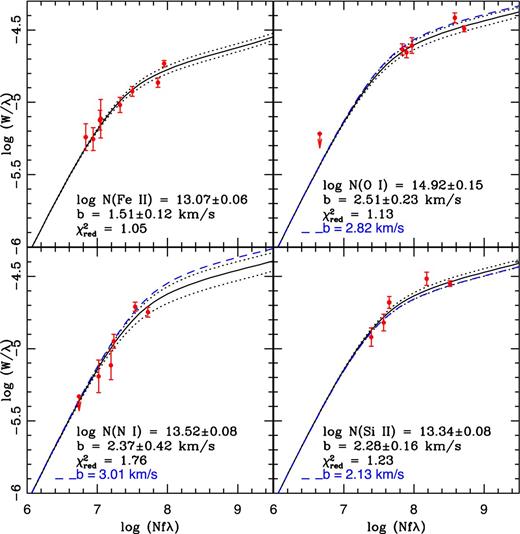
Curves of growth for the ions detected in the DLA at zabs = 2.340 06 towards J0035−0918. The black solid curves are obtained using the b estimated from our idl code, and the dotted lines show the 1σ error range. The blue dashed curves are obtained from b(|$\rm{Fe\,{\small II}}$|) under the condition of pure thermal broadening. The red points mark the observed rest-frame equivalent widths and the column densities calculated by our idl code.
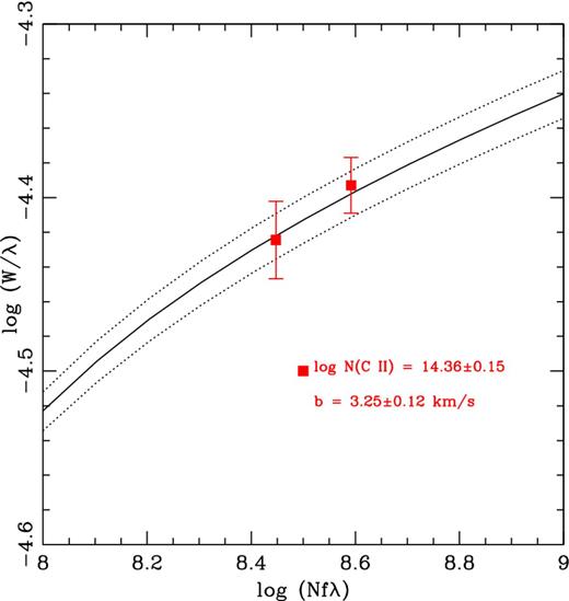
Curve of growth for |$\rm{C\,{\small II}}$| in the DLA at zabs = 2.340 06 towards J0035−0918, obtained from b(|$\rm{Fe\,{\small II}}$|). The dotted lines show the 1σ error range. The red points mark the rest-frame equivalent widths of the two |$\rm{C\,{\small II}}$| transitions. The b value used is from b(|$\rm{Fe\,{\small II}}$|) under assumption of pure thermal broadening.
Additionally, to check the results from the curve of growth method, we use vpfit to fit the metal lines covered in our UVES spectrum. First, we find that if we constrain the b parameter to be the same for all the ions (i.e. neglect the thermal broadening), a single-component cloud model with b = 2.00 ± 0.05 km s−1 fits the observed line profiles. Next, we fit the metal lines using bturb and T as independent variables for two ions of different mass (|$\rm{Fe\,{\small II}}$| and |$\rm{N\,{\small I}}$|) at the same redshift simultaneously. The chi-square for this fit is better than that for the fit considering only turbulent broadening. The best-fitting values obtained are bturb = 0.7 ± 0.5 km s−1 and T = (7.6 ± 1.9) × 103 K. These values indicate that in this case, the line widths are mainly determined by thermal broadening. In Table 3, we provide comparison of the ion column densities obtained from the two different vpfit fits and also those obtained from the curve of growth technique. The large errors in bturb, T, N(|$\rm{O\,{\small I}}$|) and N(|$\rm{C\,{\small II}}$|) that we get from vpfit are likely to be due to the low S/N of the UVES spectrum and the fact that all the |$\rm{O\,{\small I}}$| and |$\rm{C\,{\small II}}$| lines are not available to us for fitting. The values from the fit which considers both thermal and turbulent components of the Doppler parameter can be seen to agree well with those obtained from the curve of growth analysis. We find that the greatest variation in column densities, obtained by the above two methods and from the turbulence-only fit, occurs for |$\rm{O\,{\small I}}$| (∼1 dex) and |$\rm{C\,{\small II}}$| (∼2 dex). This is expected as both our |$\rm{O\,{\small I}}$| and |$\rm{C\,{\small II}}$| lines fall on the saturated part of the curve of growth, where the column density depends critically on the assumed broadening mechanism. The most important result from the comparison given in Table 3 is that the enhancement of carbon over iron (and also over oxygen) reduces drastically if we consider thermal broadening as the dominant broadening mechanism instead of turbulence. Using the curve of growth results, we get [C/Fe] = 0.36 ± 0.16, and from the best-fitting model using vpfit we obtain [C/Fe] = 0.45 ± 0.19. The C enhancement is then ∼3 times instead of ∼30 times as reported by Cooke et al. (2011a). Indeed, Carswell et al. (2012) also note the same and they report [C/Fe] = 0.51 ± 0.10 for a thermal fit to the system using vpfit, without giving any details. They obtain T = (7.66 ± 0.57) × 103 K, similar to our values; however, they get a smaller error. Here, we have carried out a detailed analysis using both curve of growth and vpfit, using more transitions of |$\rm{Fe\,{\small II}}$|. We come to the conclusion that the metal lines are most likely to be thermally broadened, and while the [C/Fe] ratio may be slightly above the range seen in metal-poor DLAs (−0.1 to 0.4) (Cooke et al. 2011b), C abundance is not more than ∼3 times that of Fe.
Column densities of ions in the DLA at zabs = 2.340 06 towards J0035−0918.
| Ion | log N (cm−2) | ||
|---|---|---|---|
| vpfit 1a | vpfit 2b | COGc | |
| |$\rm{C\,{\small II}}$| | 16.18 (0.11) | 14.45 (0.19) | 14.36 (0.15) |
| |$\rm{N\,{\small I}}$| | 13.60 (0.04) | 13.48 (0.03) | 13.52 (0.08) |
| |$\rm{O\,{\small I}}$| | 15.68 (0.18) | 14.55 (0.14) | 14.92 (0.15) |
| |$\rm{Si\,{\small II}}$| | 13.50 (0.07) | 13.37 (0.06) | 13.34 (0.08) |
| |$\rm{Fe\,{\small II}}$| | 13.01 (0.03) | 13.07 (0.04) | 13.07 (0.06) |
ab = 2.00 ± 0.05 km s−1; χ2/d.o.f. = 1010/859
bbturb = 0.89 ± 0.41 km s−1 and T = (7.3 ± 1.7) × 103 K; χ2/d.o.f. = 999/858
cCurve of growth analysis.
A value of log[N(|$\rm{H\,{\small I}}$|)(cm−2)] = 20.55 ± 0.10 is obtained for this DLA using our UVES spectrum, which is consistent with the value of Cooke et al. (2011a), and also Jorgenson, Murphy & Thompson (2013; see Fig. 3 for the fit to the DLA profile). We have derived the 3σ limiting rest-frame equivalent width for |$\rm{S\,{\small II}}$| using the strongest undetected transition (λ1259), over the full width at half-maximum obtained from our best-fitting vpfit model. We use it to calculate the upper limit to the |$\rm{S\,{\small II}}$| column density in the optically thin limit approximation (N = 1.13 × 10²⁰ W0/λ2f). Our spectrum also covers the |$\rm{Mg\,{\small II}}$| doublet λλ 2796, 2803 (see Fig. 4 for a selection of the metal line profiles). However, these lines are affected by the atmospheric absorption lines, so we can only estimate an upper limit to the column density as, log[N(|$\rm{Mg\,{\small II}}$|)(cm−2)] ≤ 13.44. We have modified the continua near the |$\rm{Si\,{\small II}}\,\lambda$|1193 and λ1260 profiles for fitting purposes. In Table 5, we present the measured column densities of some selected ions and the abundance measurements are given in Table 6. Note that the fits to the metal lines and their column densities and metallicities that we present are those from the thermal fit using vpfit.
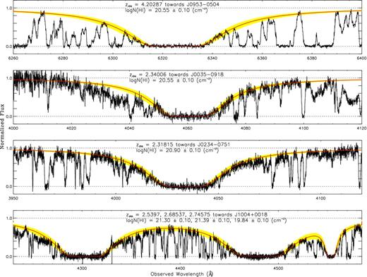
The normalized DLA profiles overplotted with the model fit to the damped Lyα absorption lines in red. The yellow shaded regions show the 1σ error in the fits. In each panel, QSO name, absorption redshift and the measured log N(|$\rm{H\,{\small I}}$|) are also quoted.
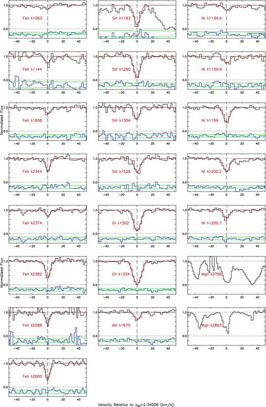
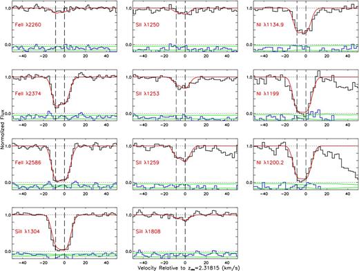
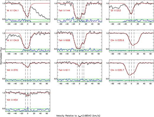
A selection of metal lines associated with the DLA at zabs = 2.340 06 towards J0035−0918. Best-fitting Voigt profiles are overplotted in red. The dashed vertical lines show the component positions. The errors in flux and residuals from the fit are shown at the bottom as green lines and blue histograms, respectively. No fit is performed for the |$\rm{Mg\,{\small II}}$| lines as these wavelength ranges are contaminated by atmospheric absorption.
From our curve of growth analysis for |$\rm{Fe\,{\small II}}$|, we get a temperature of 7600 ± 1200 K, assuming only thermal broadening. If we consider |$\rm{Fe\,{\small II}}$| and |$\rm{O\,{\small I}}$| as reference ions to solve for both temperature and bturb, we obtain T ∼ 5500 K and bturb ∼ 0.80 km s−1. These values are consistent with what is estimated by vpfit. Hence, we can conclude that for this system, the bturb is < 1.0 km s−1 and temperature lies in the range 5000 ∼ 8000 K. The temperature range is comparable to that expected in the warm neutral medium (WNM) (5000 ∼ 10 000 K) (Wolfe et al. 2003a). The high temperature is also consistent with the non-detection of |$\rm{C\,{\small II}}$|* in this system, which is most likely to arise in the cold neutral medium (CNM; Wolfe et al. 2003a; Wolfe, Gawiser & Prochaska 2003b). From the 3σ limiting rest-frame equivalent width of the |$\rm{C\,{\small II}}$|* λ 1335.71 line, we estimate log[N(|$\rm{C\,{\small II}}$|*)(cm−2)] ≤ 12.30. Since we have an estimate of temperature for this system, we model it using the photoionization software cloudy (version 07.02.02; developed by Ferland et al. 1998), as a plane-parallel slab of gas exposed to the metagalactic UV background radiation field given by Haardt & Madau (2001). In the left-hand panel of Fig. 5, we plot the temperatures estimated for different values of the neutral hydrogen density. From this figure, we can see that for temperatures ranging from 5000 to 8000 K, the density ranges from 0.8 to 0.02 cm−3, which gives length scale of the cloud between ∼4 kpc and ∼100 pc. The column density of |$\rm{C\,{\small II}}$|* predicted by the cloudy model is consistent with the upper limit estimated. We also plot the phase diagram (i.e. gas pressure versus neutral hydrogen density) predicted by the cloudy model in the right-hand panel of Fig. 5. It is clear from this figure that the observed temperature range and the inferred density range correspond to the WNM phase. Temperature estimate based on the line widths in DLAs is difficult due to blending of the velocity components, and measurements based on narrow absorption components is likely to correspond to the CNM. We note that this DLA is among the few DLAs where temperature estimation is possible and the temperature obtained from the inferred line widths is as expected in the WNM (see Carswell et al. 2012; Noterdaeme et al. 2012).
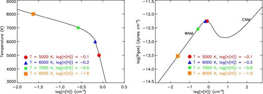
Results of photoionization calculations using N(|$\rm{H\,{\small I}}$|) and metallicity similar to the observed values for the zabs = 2.340 06 system towards J0035−0918. For the ionizing field similar to that of UV background at z ∼ zabs, the left-hand panel shows the gas temperature as a function of hydrogen density. The corresponding phase diagram is shown in the right-hand panel.
4.2 zabs = 2.318 15 towards J0234−0751
This source was picked from the SDSS data base based on the absence of strong metal lines in the spectrum. We obtain a value of log[N(|$\rm{H\,{\small I}}$|)(cm−2)] = 20.90 ± 0.06 (see Fig. 3 for the fit to DLA profile) for this system. This DLA qualifies as metal poor with [Fe/H] ∼ −2.23. The |$\rm{Fe\,{\small II}}$| abundance is well constrained by the unsaturated transitions of λ2260 and λ2374. However, the transitions of |$\rm{O\,{\small I}}\,\lambda$|1302 and |$\rm{C\,{\small II}}\,\lambda$|1334 (the only |$\rm{O\,{\small I}}$| and |$\rm{C\,{\small II}}$| lines covered by our spectrum) are both saturated. We estimate lower limits to their column densities using the optically thin limit approximation as given in Section 4.1. We notice from table 1 of Wolfe et al. (2008) that log[N(|$\rm{H\,{\small I}}$|)(cm−2)] = 20.95 ± 0.15, [M/H] = −2.74 ± 0.14 and [Fe/H] = −3.14 ± 0.04 was reported for this system without details, while table 1 of Jorgenson et al. (2013) gives log[N(|$\rm{H\,{\small I}}$|)(cm−2)] = 20.85 ± 0.10, [Si/H] = −2.46 ± 0.10 and [Fe/H] = −2.56 ± 0.04 for this system, from medium-resolution spectra, without details. While our N(|$\rm{H\,{\small I}}$|) measurement matches with that of these two cases, we disagree with their metallicity estimates.
A two component cloud model (with b parameters of 2.71 ± 0.33 and 4.29 ± 0.38 km s−1 separated by ∼8.5 km s−1) is found to fit well with the observed ion profiles (see Fig. 6 for a selection of the metal profiles). Since the metal lines are narrow, we also did a fit using bturb and T of two ions of different mass (|$\rm{Fe\,{\small II}}$| and |$\rm{N\,{\small I}}$|) as independent variables, in order to check whether there is any significant contribution from thermal broadening. However, the resulting fit was poor and the chi-square (|$\chi ^{2}_{\rm red}$| = 2.0) higher than that obtained for our best-fitting model (|$\chi ^{2}_{\rm red}$| = 1.4). Hence, we use our best-fitting result which assumes that the thermal broadening is negligible in comparison to the turbulent broadening. The details of selected ion column densities and abundances are provided in Tables 5 and 6 respectively.
Same as in Fig. 4 for a selection of metal lines associated with the DLA at zabs = 2.318 15 towards J0234−0751.
4.3 zabs = 4.202 87 towards J0953−0504
This system (also known as Q0951−0450) is part of a DLA sample used by Noterdaeme et al. (2008) to search for H2 in DLAs. For this particular sightline, we have both VLT/UVES spectrum (4780–6810 Å) and Keck/HIRES spectrum (6030–8390 Å). Almost all our lines of interest fall in the wavelength range covered by the UVES spectrum. For two transitions not covered by the UVES spectrum (|$\rm{Si\,{\small II}}\,\lambda$|1526 & |$\rm{Fe\,{\small II}}\,\lambda$|1608), we use the HIRES spectrum to fit the profiles. We derive log[N(|$\rm{H\,{\small I}}$|)(cm−2)] = 20.55 ± 0.10 for this system, which is consistent with the measurement of Noterdaeme et al. (2008). Fig. 3 shows the best-fitting Voigt profile overplotted on the Lyα profile. A two-component cloud model (with b parameters of 4.43 ± 0.28 and 5.33 ± 0.60 km s−1 separated by ∼7.5 km s−1) is found to give a good fit to the observed metal line profiles (see Fig. 7 for a selection of the metal lines). From Table 4, we can see that the component with b ∼ 4 km s−1, contains about 60 per cent of the |$\rm{C\,{\small II}}$| and |$\rm{O\,{\small I}}$|, and about 70 per cent of the |$\rm{Si\,{\small II}}$| and |$\rm{Fe\,{\small II}}$| present in the cloud.
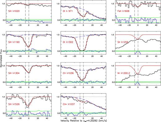
Same as in Fig. 4 for a selection of metal lines associated with the DLA at zabs = 4.202 87 towards J0953−0504. The dashed blue lines show the Lyα profiles which blend the lines of interest.
Component-wise distribution of column densities of ions in the DLA at zabs = 4.202 87 towards J0953−0504.
| Ion | log N (cm−2) | log N (cm−2) |
|---|---|---|
| Component 1 (b ∼ 4 km s−1) | Component 2 (b ∼ 5 km s−1) | |
| |$\rm{C\,{\small II}}$| | 13.68 (0.07) | 13.57 (0.09) |
| |$\rm{O\,{\small I}}$| | 14.50 (0.05) | 14.24 (0.10) |
| |$\rm{Si\,{\small II}}$| | 13.21 (0.04) | 12.80 (0.16) |
| |$\rm{Fe\,{\small II}}$| | 12.90 (0.29) | 12.60 (0.56) |
All the |$\rm{Fe\,{\small II}}$| lines except λ1608 are blended/undetected, and the error on |$\rm{Fe\,{\small II}}$| column density is relatively large since only one line in a low S/N region could be used for fitting. Even allowing for the maximum error (0.21 dex) in the metallicity measurement, this system is among one of the most metal-poor DLAs, and the most metal-poor DLA at z > 4 detected till date. However, most of the lines of interest fall in the Lyα forest and hence are blended, making identification and fitting of line profiles not straightforward. There is also another DLA along this line of sight (at zabs = 3.8567), whose metal lines sometimes contaminate our lines of interest. For the system at zabs = 4.202 87, our spectrum covers one unsaturated line each of |$\rm{O\,{\small I}}$| (λ971) and |$\rm{C\,{\small II}}$| (λ1036) (see Fig. 7). These lines allow us to derive reliable abundance measurements of O and C, respectively. The |$\rm{O\,{\small I}}\,\lambda$|971 line is in the wing of a Lyα absorption, and we fit it along with the Lyα line. We also overplot the best-fitting profile over the saturated |$\rm{O\,{\small I}}\,\lambda$|1302 line and find it to be consistent. The |$\rm{C\,{\small II}}\,\lambda$|1036 line is blended, and we fit it by assuming the contamination to be a broad Lyα. We obtain an upper limit to the |$\rm{C\,{\small II}}$|* column density by fitting the λ1037 line profile along with a Lyα profile. All the Lyα profiles which blend our lines of interest are shown in dotted blue lines in Fig. 7. Since all the |$\rm{S\,{\small II}}$| and |$\rm{N\,{\small I}}$| profiles are blended, we estimate upper limits to their column densities by overplotting profiles, obtained using the parameters from the best-fitting model, on the strongest unsaturated transition profiles (|$\rm{S\,{\small II}}\,\lambda$|1259 & |$\rm{N\,{\small I}}\,\lambda$|1200.2), and adjusting the column densities till the maximum limit. We show the absorption profiles with maximum column densities in Fig. 7. The details of selected ion column densities are presented in Table 5 and abundances are presented in Table 6.
Total column densities of selected ions in the DLAs.
| QSO | zabs | log N(|$\rm{H\,{\small I}}$|) | log N(|$\rm{C\,{\small II}}$|) | log N(|$\rm{N\,{\small I}}$|) | log N(|$\rm{O\,{\small I}}$|) | log N(|$\rm{Si\,{\small II}}$|) | log N(|$\rm{S\,{\small II}}$|) | log N(|$\rm{Fe\,{\small II}}$|) |
|---|---|---|---|---|---|---|---|---|
| (cm−2) | (cm−2) | (cm−2) | (cm−2) | (cm−2) | (cm−2) | (cm−2) | ||
| J0035−0918 | 2.340 06 | 20.55 (0.10) | 14.45 (0.19) | 13.48 (0.03) | 14.55 (0.14) | 13.37 (0.06) | ≤ 13.13 | 13.07 (0.04) |
| J0234−0751 | 2.318 15 | 20.90 (0.10) | ≥ 13.80 | 14.23 (0.03) | ≥ 14.25 | 14.32 (0.09) | 14.18 (0.03) | 14.18 (0.03) |
| J0953−0504 | 4.202 87 | 20.55 (0.10) | 13.93 (0.02) | ≤ 13.54 | 14.69 (0.02) | 13.35 (0.02) | ≤ 13.89 | 13.07 (0.19) |
| J1004+0018 | 2.539 70 | 21.30 (0.10) | ≥ 14.54 | 14.73 (0.04) | ≥ 14.91 | ≥ 14.33 | 15.09 (0.01) | 15.13 (0.02) |
| J1004+0018 | 2.685 37 | 21.39 (0.10) | ≥ 14.02 | 14.86 (0.02) | ≥ 14.54 | ≥ 13.87 | 14.70 (0.02) | 14.71 (0.04) |
| J1004+0018 | 2.745 75 | 19.84 (0.10) | ≥ 13.74 | 13.35 (0.07) | ≥ 14.25 | 13.67 (0.01) | ≤ 13.40 | 13.31 (0.02) |
Abundance measurements of selected elements in the DLAs.
| QSO | zabs | log N(|$\rm{H\,{\small I}}$|) | [C/H] | [N/H] | [O/H] | [Si/H] | [S/H] | [Fe/H] |
|---|---|---|---|---|---|---|---|---|
| (cm−2) | ||||||||
| J0035−0918 | 2.340 06 | 20.55 (0.10) | −2.53 (0.21) | −2.90 (0.10) | −2.69 (0.17) | −2.69 (0.12) | ≤−2.54 | −2.98 (0.10) |
| J0234−0751 | 2.318 15 | 20.90 (0.10) | ≥−3.53 | −2.50 (0.10) | ≥−3.34 | −2.09 (0.13) | −1.84 (0.10) | −2.22 (0.10) |
| J0953−0504 | 4.202 87 | 20.55 (0.10) | −3.05 (0.10) | ≤−2.84 | −2.55 (0.10) | −2.70 (0.10) | ≤−1.78 | −2.98 (0.21) |
| J1004+0018 | 2.539 70 | 21.30 (0.10) | ≥−3.19 | −2.40 (0.11) | ≥−3.08 | ≥−2.48 | −1.33 (0.10) | −1.67 (0.10) |
| J1004+0018 | 2.685 37 | 21.39 (0.10) | ≥−3.80 | −2.36 (0.10) | ≥−3.54 | ≥−3.03 | −1.81 (0.10) | −2.18 (0.11) |
| J1004+0018 | 2.745 75 | 19.84 (0.10) | ≥−2.53 | −2.32 (0.12) | ≥−2.28 | −1.68 (0.10) | ≤−1.56 | −2.03 (0.10) |
With [Fe/H] ≃ −3.0, this system is the only known extremely metal-poor DLA detected till date at z > 4. The relative abundance pattern of elements in this DLA is found to be similar to that of a typical metal-poor DLA (see Cooke et al. 2011b), as shown in Fig. 11. We find no enhancement of C over Fe as such ([C/Fe] = −0.07 ± 0.19). Also, C is not enhanced with respect to O ([C/O] = −0.5 ± 0.03). So like most metal-poor DLAs, typical Population II star yields will explain the abundance pattern seen in this DLA. Oxygen is found to be enhanced with respect to iron, [O/Fe] = 0.43 ± 0.20. While the present measurement is consistent with [〈O/Fe〉] = 0.35 ± 0.09 found in DLAs with −3 ≤ [Fe/H] ≤ −2 (see Cooke et al. 2011b), it is slightly lower than the mean [〈O/Fe〉] = 0.69 ± 0.14 measured for three [Fe/H] <−3 DLAs in the sample of Cooke et al. (2011b). Therefore, a possible trend of increasing [O/Fe] at [Fe/H] <−3 as suggested by Cooke et al. (2011b), requires confirmation with more measurements of these metallicities. Using the upper limit on N(|$\rm{N\,{\small I}}$|) obtained as described previously, we find that [N/O] ≤ −0.27. This lies above the primary plateau (see Section 5.2 for more details), and unfortunately we cannot come to any definite conclusions regarding the production of nitrogen in this system. Wolfe et al. (2008) have reported log[N(|$\rm{C\,{\small II}}$|*)(cm−2)] = 13.37 ± 0.08 for this system, without showing the spectrum. Our spectrum covers only the |$\rm{C\,{\small II}}$|* λ1037 line. This line is blended with a nearby Lyα absorption and our fits suggest log[N(|$\rm{C\,{\small II}}$|*)(cm−2)] ≤ 12.95 (see Fig. 7).
4.4 zabs = 2.5397, 2.685 37, 2.745 75 towards J1004+0018
This sightline contains two DLAs and one sub-DLA. They were selected on the basis of the weakness of metal lines in the SDSS spectrum. It is interesting to note that within a redshift range of ∼0.2 (Δv ∼ 17 000 km s−1) of the three systems, the [Fe/H] of the systems varies by ∼0.43 dex. The configuration of three closely spaced systems seen here is similar to the few rare cases known in the literature (Ledoux et al. 2003; Lopez & Ellison 2003; Srianand et al. 2010). It has been observed that one of the DLAs in such a configuration happens to be metal poor, which seems to be the case here as well.
We derive log[N(|$\rm{H\,{\small I}}$|)(cm−2)] = 21.30 ± 0.10 for the DLA at |$z_{\text{abs}}$| = 2.5397 (see Fig. 3). The best-fitting cloud model consists of eight components, not all present in every ion, with b parameters ranging from ∼4 to ∼12 km s−1. The metal lines show a more complex and extended component structure than that of any other systems in the present sample (see Fig. 8). Moreover, with [Fe/H] ∼ −1.7, this is the only DLA in the current study not satisfying our definition of metal poor. The presence of relatively high metallicity as well as larger velocity width of the line profiles is consistent with the velocity–metallicity relation in DLAs as observed by Ledoux et al. (2006). This being a relatively metal-rich DLA, all the transitions of |$\rm{O\,{\small I}}$|, |$\rm{C\,{\small II}}$| and |$\rm{Si\,{\small II}}$| are heavily saturated. The lower limits to their column densities have been estimated as described in Section 4.2. We also detect many transitions of |$\rm{Ni\,{\small II}}$| in this system, which are shown in Fig. 8. From our best fit, we get log[N(|$\rm{Ni\,{\small II}}$|)(cm−2)] = 13.91 ± 0.01. We give the column densities of selected ions in Table 5 and abundances in Table 6. Jorgenson et al. (2013) reports log[N(|$\rm{H\,{\small I}}$|)(cm−2)] = 21.10 ± 0.10 and [Fe/H] = −1.23 ± 0.03 for this system without details. While our N(|$\rm{H\,{\small I}}$|) measurements are consistent within errors, our metallicity estimates differ, due most likely to the medium-resolution spectrum used by Jorgenson et al. (2013).
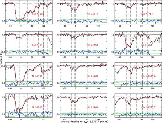
Same as in Fig. 4 for a selection of metal lines associated with the DLA at zabs = 2.5397 towards J1004+0018.
The system at |$z_{\text{abs}}$| = 2.685 37 is the second DLA along this line of sight. It has the highest neutral hydrogen column density in the present sample, with log[N(|$\rm{H\,{\small I}}$|)(cm−2)] = 21.39 ± 0.10 (see Fig. 3). Even though this is a low-metallicity system, with [Fe/H] ∼ −2.13, the strong transitions of |$\rm{O\,{\small I}}$|, |$\rm{C\,{\small II}}$| and |$\rm{Si\,{\small II}}$| covered by our spectrum are saturated. The metal line profiles are best fitted by a three-component cloud model (with b parameters between ∼4 and ∼8 km s−1), though a fourth component is required to fit the Fe profiles (see Fig. 9). |$\rm{Ni\,{\small II}}$| is detected in this system, and we obtain log[N(|$\rm{Ni\,{\small II}}$|)(cm−2)] = 13.39 ± 0.02 from our fit. The column densities (or lower limits in the case of saturated profiles) of the relevant ions are given in Table 5, while the metallicities are presented in Table 6. For this system also, the N(|$\rm{H\,{\small I}}$|) measurement reported by Jorgenson et al. (2013) (log[N(|$\rm{H\,{\small I}}$|)(cm−2)] = 21.25 ± 0.10), using medium-resolution spectrum, match with ours within errors, while their abundance measurement ([Fe/H] = −1.73 ± 0.06) differs from that obtained by us. The systems at zabs = 2.5397 and 2.685 37 are the two in our sample that clearly show |$\rm{C\,{\small II}}$|* absorption. We discuss the implications of the |$\rm{C\,{\small II}}$|* detections in Section 6.
Same as in Fig. 4 for a selection of metal lines associated with the DLA at zabs = 2.685 37 towards J1004+0018.
The sub-DLA at |$z_{\text{abs}}$| = 2.745 75 along this sightline, with [Fe/H] ∼ −2, is also a low-metallicity system. We deduce log[N(|$\rm{H\,{\small I}}$|)(cm−2)] = 19.84 ± 0.10 (see Fig. 3), and fit a two-component cloud model (with b parameters of 4.11 ± 0.48 and 5.29 ± 0.34 km s−1 separated by ∼9.3 km s−1) to the metal lines (see Fig. 10). The gas in sub-DLAs may be partially ionized; however, ionization corrections may not be very important at lower metallicities (Péroux et al. 2007). Here, we have not applied any ionization corrections while deriving the abundances. In this system also, the |$\rm{O\,{\small I}}\,\lambda$|1302 and |$\rm{C\,{\small II}}\,\lambda$|1334 lines are saturated and blended, and hence, we provide only lower limits to their column densities. We also compute the 3σ upper limit to the |$\rm{S\,{\small II}}$| column density using the strongest undetected transition (λ1259), as per the method described in Section 4.1. Table 5 lists the column densities of the relevant ions and Table 6 the respective abundances.
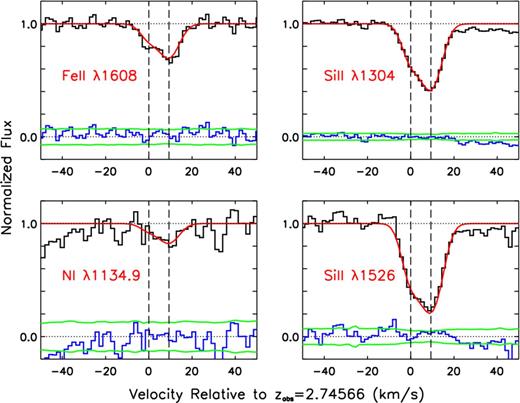
Same as in Fig. 4 for a selection of metal lines associated with the sub-DLA at zabs = 2.745 75 towards J1004+0018.
5 ELEMENTAL ABUNDANCES IN METAL-POOR DLAs
Typically, metal-poor DLAs seem to roughly follow a similar abundance pattern. Deviations in the abundance pattern are seen for CEMP DLAs, which are usually understood as enrichment by core-collapse supernovae of massive primordial stars (Kobayashi, Tominaga & Nomoto 2011). In our sample, except for the CEMP DLA towards J0035−0918, all the systems with [Fe/H] ≤ −2 seem to follow the typical relative abundance pattern of elements in a metal-poor DLA, indicating that the elemental abundances in such DLAs arise from similar population of stars. In Table 6, we list the abundances of the relevant elements in our sample, and in Fig. 11, we present a graphical comparison of the abundances measured in our systems (solid boxes) with those of a typical VMP DLA as defined by Cooke et al. (2011b, dashed boxes). We also compare the measured abundances with that of typical metal-poor stars, which we obtain by taking the average of the abundances in metal-poor stars in the halo of the Galaxy (with [Fe/H] ranging between −2.0 and −3.5), as given by Cayrel et al. (2004) and Beers & Christlieb (2005). We find that the abundance pattern of metal-poor stars (shown as stars) shows greater enhancement of C, N and O with respect to Fe than that seen till now in metal-poor DLAs, in particular, the abundance of N is more than a magnitude higher in such stars than seen in metal-poor DLAs (see Fig. 11). The top-right panel of Fig. 11 also shows the comparison of the elemental abundances in the DLA at zabs = 2.340 06 towards J0035−0918, obtained by us with that by Cooke et al. (2011a, dotted boxes). Our results are found to be consistent with theirs, except for that of carbon and oxygen. As discussed in Section 4.1, this is because while Cooke et al. (2011a) consider turbulence as the broadening mechanism behind the line widths (which is equal to assuming T = 0 K), we adopt the results obtained from thermal broadening (T ∼ 8000 K).
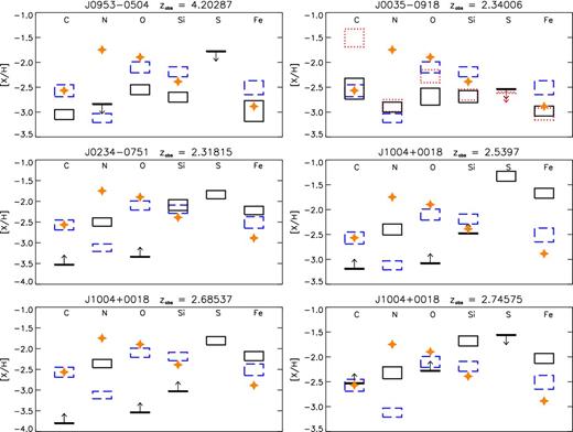
Elemental abundances in the DLAs. The height of each box represents the uncertainty in each elemental abundance. Upper and lower limits are indicated by bar and arrow. The black boxes show the abundances measured for our sample; the dashed blue boxes represent the abundance pattern of a typical VMP DLA (Cooke et al. 2011b); the dotted red boxes in the upper-right panel show the abundances of the CEMP DLA at zabs = 2.340 06 towards J0035−0918 as reported by Cooke et al. (2011a); the stars show the typical abundance pattern of metal-poor halo stars obtained from Cayrel et al. (2004) and Beers & Christlieb (2005). QSO names and absorption redshifts are provided in each panel.
In the following sections, we discuss the abundances of C, N, O in metal-poor DLAs and the overall trend of their abundance ratios as a function of metallicity, by combining our sample with that present in the literature. These elements play the most important role in the nucleosynthesis of stars, and hence studying their relative abundance patterns at low metallicity is crucial to understand the composition and yields of the first few generations of stars.
5.1 The O/Fe ratio
Oxygen is mainly produced by massive stars that undergo Type II supernova explosions (SNe II), whereas, iron is mostly (i.e. 2/3|$\text{rd}$|) produced by Type Ia supernova explosions (SNe Ia) of low- and intermediate-mass stars. Since low- and intermediate-mass stars take longer time to evolve than massive stars, SNe Ia occur ∼1 Gyr later than SNe II. Therefore, initially at low metallicity, oxygen is expected to be enhanced relative to iron. Later, when the delayed contribution to iron by SNe Ia starts, the O/Fe ratio is expected to decrease. Thus, the relative abundance of O and Fe is a good indicator of the relative contribution of SNe Ia and SNe II yields towards chemical enrichment, as well as the time delay between them. Additionally, at low metallicity the O/Fe ratio can serve as a measure of the relative production of α to iron-peak elements by the early generations of high-mass stars.
The measurement of oxygen abundance in DLAs is usually an issue, since the stronger |$\rm{O\,{\small I}}$| lines are mostly saturated and the weaker ones are often blended within the Lyα forest. As can be seen from Table 6, we have direct measurement of the oxygen abundance for only two DLAs. For the DLA at zabs = 2.340 06 towards J0035−0918, we get [O/Fe] = 0.29 ± 0.15, while for the other DLA at zabs = 4.202 87 towards J0953−0504, we find [O/Fe] = 0.43 ± 0.20. These are among the four measurements of oxygen in DLAs with [Fe/H] ≤ −2.9. Our values do not seem to imply an upward trend of [O/Fe] at [Fe/H] < −3.0, as hinted at by Cooke et al. (2011b); however, more data are required to reach any definite conclusions. For remaining systems, we use S (or Si) as proxy to O abundance measurements using solar abundances (abundances of S and Si follow that of O, all being α-capture elements). The average [〈O/Fe〉] for the five systems in our sample with [Fe/H] ≤ −2.0 is 0.36 ± 0.26. This is consistent with the average [〈O/Fe〉] = 0.35 ± 0.09 found in DLAs with −3 ≤ [Fe/H] ≤ −2, as well as the [〈O/Fe〉] ∼ 0.4 seen in metal-poor stars with −3.5 ≤ [Fe/H] ≤ −1 (Cooke et al. 2011b). The [O/Fe] ratios for our sample are shown in the top-right panel of Fig. 12, along with those for VMP DLAs in the literature, as well as for metal-poor halo stars as given in Cooke et al. (2011b), for comparison. It has been shown that DLAs typically exhibit minimal dust depletion when [Fe/H] ≲ −2.0 (Ledoux et al. 2003; Vladilo 2004; Akerman et al. 2005). Cayrel et al. (2004) find constant [Si/Fe] ∼ 0.37 from the measurements of metal-poor stars in the halo of the Galaxy, indicating that at lower metallicities the intrinsic nucleosynthetic Si/Fe ratio is almost independent of the metallicity. For our present sample, we find that [〈Si/Fe〉] ∼ 0.34, consistent with that found by Cayrel et al. (2004).
![Top right: the [O/Fe] ratio versus [Fe/H] in our DLAs compared with that of VMP DLAs and metal-poor stars as compiled by Cooke et al. (2011b). Top left: the [N/O] ratio versus [O/H] in our DLAs compared with that of DLAs and local measurements as given by Petitjean et al. (2008) and Cooke et al. (2011b) and sources cited by them. Bottom: the [C/O] ratio versus [O/H] in our DLAs compared with that of VMP DLAs and metal-poor stars as compiled by Cooke et al. (2011b).](https://oup.silverchair-cdn.com/oup/backfile/Content_public/Journal/mnras/440/1/10.1093_mnras_stu260/2/m_stu260fig12.jpeg?Expires=1716405829&Signature=31h8OM6D6KxH-z~4kClIkeApspPyv4Nl351duVHA4KijiHaHnmu0rk5s~eQu4CcstnPNwzxmK4e4c~0tlOzlbs1Zp0YXNSNtOdnR9urBKY6fuvRz6nWR7oAMAXXBxdRKXCNkza6xgMZlybKWCQYuCIOPRc7kflgiO5laGe5ld6FzAC1rH6Lp19j1L~vuzAfTCGhE3k7OqEad2k61EMLB6UProDxyLq-kxUJeUjLSeA9gts6nbShM-9nzurRum9p1S-1IZNbInhikRBcFx5hPot2eBuxJGZvtui-XACnl9ReeRkpZeJGLyXfAoDsPflJw5i0WN0zWzi4etvJFJz6SXw__&Key-Pair-Id=APKAIE5G5CRDK6RD3PGA)
Top right: the [O/Fe] ratio versus [Fe/H] in our DLAs compared with that of VMP DLAs and metal-poor stars as compiled by Cooke et al. (2011b). Top left: the [N/O] ratio versus [O/H] in our DLAs compared with that of DLAs and local measurements as given by Petitjean et al. (2008) and Cooke et al. (2011b) and sources cited by them. Bottom: the [C/O] ratio versus [O/H] in our DLAs compared with that of VMP DLAs and metal-poor stars as compiled by Cooke et al. (2011b).
5.2 The N/O Ratio
Nitrogen is mainly produced through the CNO cycle in hydrogen burning layers of stars. It is believed to be of both primary and secondary origin, depending on whether the seed C and O are produced by the star itself during helium burning (primary), or whether they are leftovers from earlier generations of stars and hence already present in the interstellar medium (ISM) from which the star formed (secondary). Primary N is thought to be generated by intermediate-mass stars on the asymptotic giant branch (AGB). Secondary N is produced by all stars as C and O are present in their H burning layers. In |$\rm{H\,{\small II}}$| regions of nearby galaxies, it has been observed that the N/O ratio rises steeply with increasing oxygen abundance for [O/H] ≳ −0.4; this is the secondary regime. At lower metallicity, for [O/H] ≲ −0.7, the N/O ratio remains constant; this is the primary regime where N abundance tracks that of O.
The measurement of N/O ratio in DLAs is again complicated by the fact that the |$\rm{O\,{\small I}}$| absorption lines are either saturated or blended, while the |$\rm{N\,{\small I}}$| lines may be blended in the Lyα forest. Here, we adopt the standard practice of replacing O abundance by that of another α element S (or Si), whenever measurement of O is not available. In upper-right panel of Fig. 12, we plot the [N/O] ratio versus O abundance for our sample, as well as values reported by Petitjean et al. (2008) and Cooke et al. (2011b). We also show the location of the local primary plateau ([N/O] between −0.57 and −0.74) and secondary production region (extrapolated from local measurements), as given by Petitjean et al. (2008). Most of the DLA values lie within these two regions, which may imply that the DLAs are in the transition period following a burst of star formation, when the ISM has been enriched by O released from SNe II, but lower mass stars have yet to release their primary N. To this group belongs the system at zabs = 2.5397 towards J1004+0018 studied here. In one of the two cases (zabs = 4.202 87 towards J0953−0504) where we have O measurement, we could only get upper limit on N(|$\rm{N\,{\small I}}$|). This suggests [N/O] ≤ −0.29, which is above the primary plateau. So nothing definitive can be said about the relative enrichment of N and O in this system. For the system at zabs = 2.340 06 towards J0035−0918, we get [N/O] = −0.21 ± 0.14. This lies above the local primary plateau, i.e. the amount of nitrogen relative to oxygen in this system is higher than what is seen in typical DLAs. Note that this is the CEMP VMP DLA whose abundance pattern shows deviations from that of a typical VMP DLA (see Fig. 11). The [N/O] ratio for three of the remaining systems (where we have used S or Si as proxy for O) falls along the primary plateau. The high N/O ratios in these systems indicate that the release of primary N by intermediate-mass AGB stars into the ISM has caught up with that of O by massive stars.
5.3 The C/O ratio
The evolution of the [C/O] ratio with O abundance has been studied by Akerman et al. (2004) for halo stars, who found that [C/O] rises from ∼−0.5 to solar when [O/H] ≳ −1. This is interpreted as the additional contribution to C, from massive stars whose mass-loss rates increase with metallicity, and less importantly, from low- and intermediate-mass stars that take longer to evolve than massive stars. More interestingly, Akerman et al. (2004) found an increasing trend of [C/O] with decreasing metallicity when [O/H] ≲ −1, suggesting that [C/O] may reach near-solar values when [O/H] ≲ −3. This trend of rising [C/O] with decreasing O abundance has also been observed in low-metallicity DLAs by Pettini et al. (2008), Penprase et al. (2010) and Cooke et al. (2011b), indicating the enhancement of C over O in this regime may have a universal origin. Models of Population II nucleosynthesis predict that below [O/H] ∼ −1, [C/O] decreases (or perhaps flattens) with decreasing metallicity (due to time lag in C production relative to O), in contrast to the observed trend.
The upward trend in [C/O] with decreasing metallicity can be explained either as signatures of high carbon production by the first generation Population III stars, or as increased carbon yield from rapidly rotating low-metallicity Population II stars. Fig. 12 (bottom panel) shows the [C/O] ratio versus [O/H] for metal-poor stars and DLAs as given in Cooke et al. (2011b). Oxygen and carbon both have very strong transitions which are usually saturated in DLAs. In the present study, we have reliable abundance measurement of O and C in only two systems, which we show in Fig. 12. For the DLA at zabs = 4.202 87 towards J0953−0504, the abundance of O is low ([O/H] ≲ −2.5); however, C is not enhanced with respect to O ([C/O] = −0.5 ± 0.03). At least in this system, abundances of C and O are not following what is expected in the case of chemical evolution dominated by Population III stars. No DLA has been observed with super-solar [C/O], apart from the system (towards J0035−0918) reported by Cooke et al. (2011a) and also analysed here. However, as discussed in Section 4.1, the [C/O] ratio obtained by us is 0.16 ± 0.25, about four times less than 0.77 ± 0.17 obtained by Cooke et al. (2011a). While the amount of enhancement that we find is smaller compared to that reported by Cooke et al. (2011a), the enhancement of C still indicates that the gas in this system may have been enriched by yields of Population III stars.
6 |$\rm{C\,{\small II}}$|* IN METAL-POOR DLAs
We observe |$\rm{C\,{\small II}}$|* λ1335 absorption in two of our systems, along the sightline J1004+0018: log[N(|$\rm{C\,{\small II}}$|*)(cm−2)] = 13.63 ± 0.02 in the DLA at zabs = 2.5397 (hereafter DLA1); and log[N(|$\rm{C\,{\small II}}$|*)(cm−2)] = 13.94 ± 0.03 in the DLA at zabs = 2.685 37 (hereafter DLA2). For DLA1, we compute log(|$l_{\text{c}}$|) to be −27.19 ± 0.10 ergs s−1 H−1, while it is −26.97 ± 0.10 for DLA2 (see Table 7). These values fall in the trough of the bimodal distribution of |$l_{\text{c}}$| in DLAs as reported by Wolfe et al. (2008). They propose two separate populations of DLAs: ‘low cool’ DLAs with |$l_{\text{c}} \le l_{\text{c}}^{\text{crit}}$| and ‘high cool’ DLAs with |$l_{\text{c}} > l_{\text{c}}^{\rm crit}$| (|$l_{\text{c}}^{\rm crit} \simeq$| 10−27 ergs s−1 H−1). Both these populations need local radiation in excess of the UV background. While ‘low cool’ DLAs are consistent with gas embedded in a region with in situ star formation, ‘high cool’ DLA gas may be related to the outskirts of star-forming galaxies.
It is well known, for the range of densities seen in the neutral ISM, dust photoelectric heating, CR heating, X-ray heating and heating by |$\rm{C\,{\small I}}$| ionization are the dominant heating processes (Wolfire et al. 1995). Wolfe et al. (2003a) have shown that for the N(|$\rm{H\,{\small I}}$|) typically seen in DLAs, the X-ray heating is sub-dominant compared to the grain photoelectric heating and the CR heating. To understand the importance of these physical processes in the present low-metallicity systems, we construct photoionization models using cloudy.
We model the DLAs as plane-parallel slabs of gas of constant density exposed to different radiation fields: metagalactic UV background radiation given by Haardt & Madau (2001) and the ISM radiation field in-built in cloudy (i.e. spectral energy distribution given in ‘Table ISM’). We consider a range of local ionizing radiation by scaling the ISM radiation with a scale factor (with the strength of unscaled ISM radiation field G0 corresponding to a flux of 1.6 × 10⁻³ erg cm−2s−1). In Fig. 13, we show the two ionizing spectra used in our models. Note when we scale the ISM field, the UV as well as X-ray background scales by the same factor. Inclusion of CRs is very important as they are known to influence the ionization and chemical state of high-density ISM. We also include the CR background (as seen in the Galaxy) that corresponds to an H0 ionization rate of 2.5 × 10⁻¹⁷ s−1. For simplicity, we scale the CR background by the same amount as UV background in our models. In the case of models with Haardt & Madau background, we include the CR background that is 1/10|$\text{th}$| of the Galactic CR background. Note that, we use the extinguish command of cloudy to take into account extinction due to photoelectric absorption by a cold neutral slab with N(|$\rm{H\,{\small I}}$|) = 1021 cm−2. This is the standard procedure used to model ISM sightlines (Shaw et al. 2006). The cosmic microwave background at any particular redshift is also included.
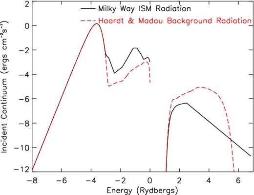
The incident continuum spectra used in our photoionization models.
For most of the results of photoionization models presented below, we consider radiation field to be impinging on one side of the cloud and our line of sight to be perpendicular to the slab (i.e. N(|$\rm{H\,{\small I}})^{\perp }$| = N(|$\rm{H\,{\small I}}$|) observed). However, in the end we discuss the results of relaxing these conditions. We also discuss what happens if we assume the absorbing gas to be a parallel slab with constant pressure.
6.1 Photoionization model for two systems with |$\rm{C\,{\small II}}$|* detections
We construct the phase diagrams for the DLAs (gas pressure versus hydrogen number density n(H); see panels a of Figs 14 and 15), by varying the n(H) and stopping the simulations when N(|$\rm{H\,{\small I}}$|) becomes equal to that observed in the DLAs. Results for Haardt & Madau radiation field as well as the local radiation field scaled by different scale factors are also plotted. We put constraints on n(H) of the DLAs using the observed |$\rm{C\,{\small II}}$|* cooling rate and N(|$\rm{C\,{\small II}}$|*)/N(|$\rm{S\,{\small II}}$|) (panels b and c of Figs 14 and 15, respectively). We use the 3σ upper limit of N(|$\rm{C\,{\small I}}$|) as consistency checks on our models (panels d of Figs 14 and 15). From the results of the simulations, we observe that:
For both systems, the extragalactic UV background radiation alone is not sufficient to produce the observed amount of |$\rm{C\,{\small II}}$|*, and a local radiation field (due to active star formation) is required to produce the |$\rm{C\,{\small II}}$|* observations (consistent with that found by Wolfe et al. 2003a, 2008).
The observed |$l_{\text{c}}$| and N(|$\rm{C\,{\small II}}$|*)/N(|$\rm{S\,{\small II}}$|) are reproduced with the ISM radiation field scaled by factor between 1–2 and log n(H) (cm−3) = 0.7 ± 0.3 for DLA1, and the ISM field scaled by factor between 2–4 and log n(H) (cm−3) = 1.50 ± 0.20 for DLA2. As can be seen from the panels (a) of Figs 14 and 15, such conditions satisfy a stable CNM phase. Note that in typical VMP DLAs, C is slightly underabundant with respect to Si ([C/Si] ∼ −0.2; see Fig. 11), while cloudy assumes solar composition. To account for this, we have included 0.2 dex in the upper bound on the observed N(|$\rm{C\,{\small II}}$|*)/N(|$\rm{S\,{\small II}}$|) for the DLA2 which is a low-metallicity DLA.
We note that the above solutions are consistent with the observed upper limits of N(|$\rm{C\,{\small I}}$|)/N(|$\rm{C\,{\small II}}$|*) (see panels d Figs 14 and 15). The constraints could be better if we had high enough resolution to detect |$\rm{C\,{\small I}}$|. Furthermore, we checked that our models do not produce any |$\rm{C\,{\small iv}}$| and |$\rm{Si\,{\small iv}}$|. While we do detect these high ions in our systems, they are shifted in velocity space with respect to the first ions and neutral species, indicating that they are most probably associated with a distinct phase (Fox et al. 2007). Our models also do not produce any |$\rm{Si\,{\small III}}$| and |$\rm{Al\,{\small III}}$|. |$\rm{Si\,{\small III}}$| line is heavily blended in both the DLAs, and hence not an useful constraint. Our spectrum does not cover |$\rm{Al\,{\small III}}$| line for both the DLAs. Note that the presence of |$\rm{Al\,{\small III}}$| along with the absence of |$\rm{C\,{\small I}}$| would be inconsistent with |$\rm{C\,{\small II}}$|* absorption originating from the CNM (Srianand et al. 2005). Hence, detection of |$\rm{Al\,{\small III}}$| in these systems would imply that the |$\rm{C\,{\small II}}$|* absorption is arising from the warm/partially ionized gas.
For both the above stable CNM solutions, heating due to CRs dominates the total heating rate. This is demonstrated in Fig. 16. In the top panel, we show heating & cooling rates from the best-fitting photoionization model for the DLA1. It is clear from this figure that, in the density range constrained by the observations, |$\rm{C\,{\small II}}$|* dominates the net cooling rate and CR heating accounts for ∼60 per cent of the total heating rate. This is the case also for DLA2 (see the bottom panel in Fig. 16). The additional heating one sees for log n(H) ≥ 2 is due to heating by collisional deexcitations of vibrationally excited H2 molecules that are present in our models. This process cannot be dominant in our systems as H2 molecules are not detected. In summary, the observed |$\rm{C\,{\small II}}$|* in two DLAs in our sample are consistent with the gas being CNM, heated mainly by CRs.
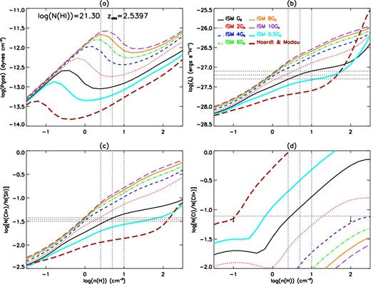
(a) Phase diagrams, (b) |$\rm{C\,{\small II}}$|* cooling rates, (c) N(|$\rm{C\,{\small II}}$|*)/N(|$\rm{S\,{\small II}}$|) and (d) N(|$\rm{C\,{\small I}}$|)/N(|$\rm{C\,{\small II}}$|*) from cloudy for the DLA at zabs = 2.5397 towards J1004+0018, for various ionizing backgrounds. The horizontal dashed lines indicate the observed values (upper limit in d) along with the errors. The vertical dashed lines indicate the expected n(H) along with errors for a CNM solution obtained from the observed |$l_{\text{c}}$| and N(|$\rm{C\,{\small II}}$|*)/N(|$\rm{S\,{\small II}}$|).
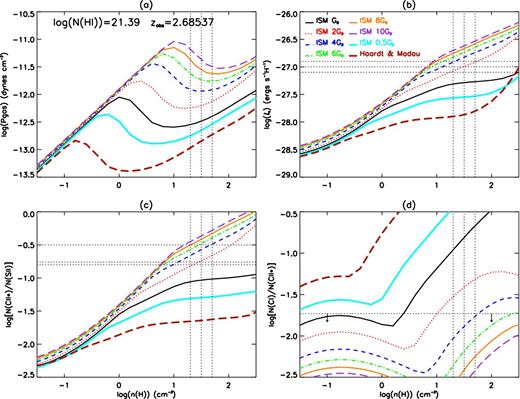
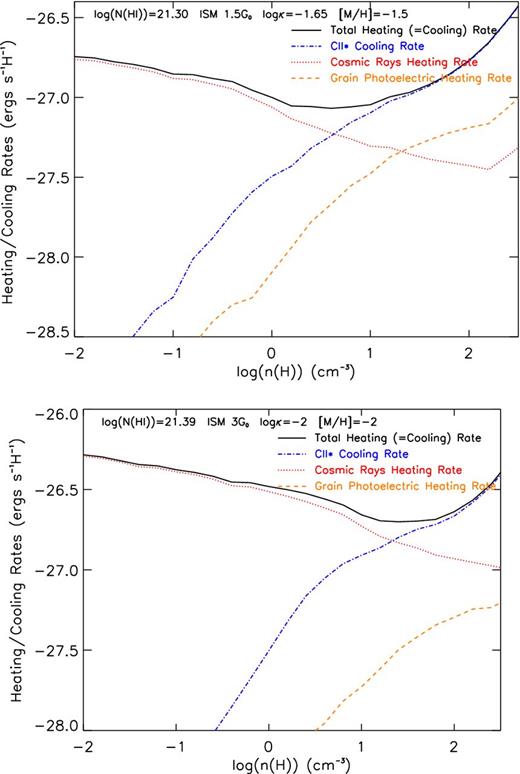
Heating and cooling rates from our photoionization models for the DLAs at zabs = 2.5397 (top) and 2.685 37 (bottom) towards J1004+0018.
Higher radiation field is required to produce the observed |$\rm{C\,{\small II}}$|* absorption in DLA2 (having lower metallicity and dust-to-gas ratio) than in DLA1. However, converting this UV field into a SFR is not straightforward as UV field not only depends on SFR but also on the mean ISM opacity. In the low-metallicity, low-dust case, we expect the mean free path for dust scattering to be larger and hence a higher UV radiation field even when the SFR is low. However, we find that the main heating source in these DLAs are CRs. We require the CR background 1–2 times and 2–4 times that of what is seen in the Milky Way for DLA1 and DLA2, respectively.
The CR heating rate can be taken as proportional to the supernova rate, since CRs are accelerated in supernova shock fronts, and hence related to the SFR (see equation 9 of Wolfe et al. 2003a). If we follow this argument, then we can conclude that the present SFR in DLA1 and DLA2 are 1–2 times and 2–4 times that of the Milky Way, respectively. Therefore, despite the gas phase metallicity being low in these systems, the required heating rate suggests that there is ongoing star formation activity in these systems.
Note that the cloudy models presented above assume one-sided illumination. We also ran test models assuming illumination from both the sides (using ‘double’ command of cloudy) to check for differences. We find that that N(|$\rm{C\,{\small II}}$|*)/N(|$\rm{S\,{\small II}}$|) and |$l_{\text{c}}$| are slightly higher in the latter case, but the differences are ≲0.1 dex and within the errors of the observed values of N(|$\rm{C\,{\small II}}$|*)/N(|$\rm{S\,{\small II}}$|) and |$l_{\text{c}}$| used to constrain the models. Hence, the n(H) values and radiation field that we obtained from our best-fitting models hold true in the latter case also.
All our models assume constant density throughout the absorbing cloud. As a check, we also ran constant pressure models for a few cases. We find that the hydrogen density and temperature profiles do not change much (≲0.1 dex) throughout the structure of the cloud, for initial n(H) corresponding to the WNM and the CNM. However, for initial n(H) corresponding to the unstable phase, the density and temperature drop by ∼1 dex across the cloud. As shown earlier, the observed quantities in the DLAs are well reproduced by stable CNM models. Then for initial n(H) corresponding to the average n(H) of the CNM models, there are no significant changes in the results of the constant pressure models from that of the constant density models.
Note that in all our model predictions, the column densities are obtained assuming our line of sight is perpendicular to the plane-parallel slab. To check for inclination effects, we ran models assuming that the absorbing slab is tilted with respect to the sightline (i.e. N(|$\rm{H\,{\small I}})^{\perp }$| = |$\text{cos}(\theta ) \;\times$|N(|$\rm{H\,{\small I}}$|) observed, with θ being the inclination angle). In order to consider this, we took the stopping N(|$\rm{H\,{\small I}}$|) of the slab as the observed value multiplied by the average value of cosine (i.e. 0.5). We find that this reduction in N(|$\rm{H\,{\small I}}$|) has no effect on the results of the models, and CRs are still the dominant heating agents required to explain the observed quantities in the DLAs.
6.2 |$\rm{C\,{\small II}}$|* in low-metallicity DLAs
In Table 7, we give the limits or in case of detection, the values of column densities and cooling rates of |$\rm{C\,{\small II}}$|* measured for the DLAs in our sample. We found a total 39 DLAs in the literature with [Fe/H] ≤ −2.0 for which the column density of |$\rm{C\,{\small II}}$|* or an upper limit to it has been measured (Wolfe et al. 2003a, 2008; Srianand et al. 2005; Noterdaeme et al. 2008; Cooke et al. 2011b). In 26 systems, |$\rm{C\,{\small II}}$|* is not detected, and we summarize the basic properties of the remaining 13 systems in Table 8. We notice that there is no difference in the distribution of metallicity between the systems with and without |$\rm{C\,{\small II}}$|*. However, systems with |$\rm{C\,{\small II}}$|* detections tend to have higher N(H i) (with a median value of log[N(H i)(cm−2)] = 20.9), compared to those without |$\rm{C\,{\small II}}$|* detection (with a median value of log[N(H i)(cm−2)] = 20.5).
Measurements of |$\rm{C\,{\small II}}$|* and cooling rates in DLAs in our sample.
| QSO | zabs | log N(|$\rm{H\,{\small I}}$|) | log N(|$\rm{C\,{\small II}}$|*) | log |$l_{\text{c}}$| | [Fe/H] | [M/Fe] | M |
|---|---|---|---|---|---|---|---|
| (cm−2) | (cm−2) | (ergs s−1 H−1) | |||||
| J0035−0918 | 2.340 06 | 20.55 (0.10) | ≤ 12.30 | ≤−27.77 | −2.98 (0.10) | 0.29 (0.09) | Si |
| J0234−0751 | 2.318 15 | 20.90 (0.10) | ≤ 12.37 | ≤−28.05 | −2.22 (0.10) | 0.38 (0.06) | S |
| J0953−0504 | 4.202 87 | 20.55 (0.10) | ≤ 12.95 | ≤−27.12 | −2.98 (0.21) | 0.28 (0.19) | Si |
| J1004+0018 | 2.539 70 | 21.30 (0.10) | 13.63 (0.02) | −27.19 (0.10) | −1.67 (0.10) | 0.34 (0.02) | S |
| J1004+0018 | 2.685 37 | 21.39 (0.10) | 13.94 (0.03) | −26.97 (0.10) | −2.18 (0.11) | 0.37 (0.03) | S |
| J1004+0018 | 2.745 75 | 19.84 (0.10) | ≤ 12.28 | ≤−27.08 | −2.03 (0.10) | 0.35 (0.02) | Si |
List of metal-poor DLAs in the literature with |$\rm{C\,{\small II}}$|* detection.
| QSO | zabs | log N(|$\rm{H\,{\small I}}$|) | log N(|$\rm{C\,{\small II}}$|*) | log |$l_{\text{c}}$| | [Fe/H] | [M/Fe] | log N(|$\rm{C\,{\small II}}$|*)/N(|$\rm{S\,{\small II}}$|) | Ref. |
|---|---|---|---|---|---|---|---|---|
| (cm−2) | (cm−2) | (ergs s−1 H−1) | ||||||
| J001328.21+13582 | 3.2811 | 21.55 (0.15) | 13.67 (0.04) | −27.40 (0.16) | −2.72 (0.02) | 0.62 (0.16) | −0.90 (0.07) | 1 |
| SDSS0127−00 | 3.7274 | 21.15 (0.10) | 13.20 (0.06) | −27.47 (0.12) | −2.90 (0.02) | 0.50 (0.10) | ≤−0.72 | 1 |
| PSS0133+0400 | 3.6919 | 20.70 (0.10) | 12.95 (0.03) | −27.27 (0.11) | −2.74 (0.05) | 0.40 (0.16) | ≤−0.92 | 1 |
| J0255+00 | 3.9146 | 21.30 (0.05) | 13.44 (0.04) | −27.38 (0.06) | −2.05 (0.09) | 0.27 (0.09) | −1.28 (0.04) | 1 |
| J0311−1722 | 3.7340 | 20.30 (0.06) | 13.55 (0.06) | −26.27 (0.08) | ≤−2.01 | ≥−0.49 | 0.63 (0.09) | 2 |
| FJ0747+2739 | 3.9000 | 20.50 (0.10) | 13.35 (0.07) | −26.67 (0.12) | −2.45 (0.03) | 0.44 (0.03) | −0.29 (0.07) | 1 |
| PC0953+47 | 4.2442 | 20.90 (0.15) | 13.60 (0.10) | −26.82 (0.18) | −2.52 (0.08) | 0.33 (0.09) | −0.25 (0.10) | 1 |
| J120802.65+63032 | 2.4439 | 20.70 (0.15) | 13.55 (0.03) | −26.67 (0.15) | −2.55 (0.01) | 0.23 (0.15) | 0.05 (0.04) | 1 |
| Q1337+11 | 2.7959 | 20.95 (0.10) | 13.11 (0.10) | −27.36 (0.14) | −2.03 (0.08) | 0.31 (0.14) | −1.16 (0.11) | 1 |
| J1340+1106 | 2.7958 | 21.00 (0.06) | 12.99 (0.04) | −27.53 (0.07) | −2.15 (0.06) | 0.32 (0.09) | −1.30 (0.04) | 2 |
| BRI1346−03 | 3.7358 | 20.72 (0.10) | 12.55 (0.11) | −27.69 (0.15) | −2.63 (0.02) | 0.30 (0.02) | −1.01 (0.11) | 1 |
| J203642.29−05530 | 2.2805 | 21.20 (0.15) | 13.36 (0.08) | −27.36 (0.17) | −2.24 (0.02) | 0.53 (0.17) | −1.25 (0.11) | 1 |
| J231543.56+14560 | 3.2729 | 20.30 (0.15) | 13.55 (0.08) | −26.27 (0.17) | −2.03 (0.03) | 0.25 (0.15) | −0.09 (0.09) | 1 |
From Table 8, we note that 8 of the 13 DLAs from the literature sample, and all the systems in our sample (within errors) fall in the ‘low cool’ category of the bimodal distribution as defined by Wolfe et al. (2008). The fraction of ‘low cool’ DLAs we find among the |$\rm{C\,{\small II}}$|* detections is much higher than that seen in the DLA sample of Wolfe et al. (2008). It is also clear from the table that the typical value of log N(C ii*)/N(S ii) is −1.0 and ≥−0.3, respectively, for the ‘low cool’ and ‘high cool’ DLAs, respectively.
To draw some broad conclusions, we construct photoionization models considering the median properties of the DLAs in Table 8. We use log N(H i) = 20.90, [M/H] = −2.2 and log κ = −2.4 in cloudy. The results for four values of the ionizing radiation are given in Fig. 17. In the bottom panel, we show the model predicted values of log N(C ii*)/N(S ii). It is clear from the figure that log N(C ii*)/N(S ii) ∼ −1 is obtained for radiation field (and CR ionization rate) similar to what is seen in the Galaxy with n(H i) ∼ 10 cm−3. For log N(C ii*)/N(S ii) ≥−0.3 as found in the case of ‘high cool’ metal-poor DLAs, one requires the radiation field (and CR ionization rate) to be at least more than four times that seen in the Galaxy and n(H i) ≥ 60 cm−3. We also find in all these cases that the CR heating dominates the gas heating rate. If we use a simple relation between SFR and CR ionization rate, then the SFR in these metal-poor DLAs are similar to or higher than what is seen in the Milky Way. In the models discussed above, we use [C/S] as in solar composition. From table 11 of Cooke et al. (2011b), we can see [C/Si] is ∼−0.20 in DLAs with carbon detection. If indeed C is slightly underabundant compared to S, then we will require higher density and higher CR ionization rate compared to what we derive above. Based on the observed high J excitations of H2 in DLAs, it has been inferred that UV radiation field similar to or higher than the mean Galactic UV background is required in these systems (Hirashita & Ferrara 2005; Srianand et al. 2005). However, these systems usually have at least an order of magnitude higher metallicity and dust compared to the low-metallicity DLAs (see for e.g. Petitjean et al. 2006). Hence, irrespective of the metallicity, it seems that the inferred background radiation is similar to or higher than that of the Galaxy, whenever one uses indirect tracers to study the physical conditions in DLAs. However, the most challenging task is to convert this background radiation to the SFR.
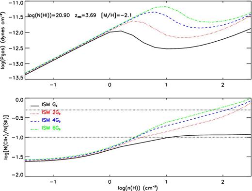
Results of photoionization model having the median property of the low-metallicity DLAs listed in Table 8. Top panel shows the phase diagram and in the bottom panel log N(C ii*)/N(S ii) is plotted against hydrogen density.
The requirement of ongoing star formation at a reasonable rate in a VMP DLA is similar to that required to explain the observations of the blue compact dwarf galaxy I Zw 18 in the local Universe (Annibali et al. 2013). In this case, it has been suggested that either the star formation is less efficient in populating the galaxy with metals or galactic winds have removed metals created in previous cycles of star formation. The same can be applicable to the high-z low metal DLAs showing signatures of ongoing star formation. Detecting the host galaxies of DLAs will be interesting to study the nature of star formation and magnetic fields (required for the generation and confinement of CRs) in VMP gas at high-z.
7 SUMMARY AND CONCLUSIONS
We have studied a sample of five DLAs and one sub-DLA and obtained their elemental abundances. Four of these DLAs and the sub-DLA turn out to be metal poor, with [Fe/H] ≲ −2.0, and among these DLAs, two are extremely metal poor, with [Fe/H] ≃ −3.0. One of the extremely metal-poor systems (zabs = 2.340 06 towards J0035−0918) studied here has also been analysed by Cooke et al. (2011a). This is also one of the two instances of CEMP DLAs that have been detected. However, we find that the extremely large enhancement of C in this system, as reported by Cooke et al. (2011a), is most probably due to the b parameter being constrained to be the same for both the high- and low-mass ions, or in other words neglecting the thermal broadening. From our curve of growth analysis and the best fit to the metal line profiles using vpfit, we come to the conclusion that the line widths are likely to be determined by thermal broadening. In this case, carbon is still enhanced over iron, but by about three times. We estimate the DLA to have temperature in the range of 5000–8000 K. Using this and from our cloudy model, we find that the physical conditions in this gas are consistent with a WNM in ionization equilibrium with the metagalactic UV radiation field dominated by the QSOs and galaxies.
The system at zabs = 4.202 87 towards J0953−0504 is the most metal-poor DLA at z > 4 studied till date. It shows no enhancement of carbon or oxygen and its relative elemental abundance pattern is similar to that of a typical metal-poor DLA, which may be explained by standard Population II nucleosynthesis results. The O/Fe, N/O and C/O ratios measured for our full sample conform to the observed trends seen in other metal-poor DLAs and stars.
In addition, we have studied the cooling and heating processes in two of the DLAs showing |$\rm{C\,{\small II}}$|* absorption using cloudy. The |$\rm{C\,{\small II}}$|* absorption is found to arise in the CNM phase and accounts for ≳80 per cent of the total cooling in the DLAs. For the CNM solution, heating by CRs is found to contribute ∼60 per cent to the total heating in the DLAs. Further, we find that an intergalactic background radiation field is not sufficient to produce the observed |$\rm{C\,{\small II}}$|* cooling in the DLAs, implying in situ star formation in the DLAs, which is the same conclusion as reached by Wolfe & Chen (2006) and Wolfe et al. (2008). We infer the radiation field (in particular the CR ionization rate) in the DLAs to be similar to the local ISM with amplitude scaled by some factor (G0 ranging from 1 to 4 times that of the Galaxy).
Lastly, we have assembled a sample of DLAs with [Fe/H] ≤ −2.0 and showing |$\rm{C\,{\small II}}$|* absorption from the literature. Using photoionization models, we argue that in such low-metal and low-dust systems, heating by grains is not as effective as in the Galactic ISM, and CRs are most probably responsible for the observed excitation of |$\rm{C\,{\small II}}$|*. The inferred CR ionization rate varies from same as (in the case of ‘low cool’ metal-poor DLAs) to more than four times (in the case of ‘high cool’ metal-poor DLAs) that seen in the Milky Way. Understanding this high CR-ionizing rate in the metal-poor DLAs will enable us to understand star formation history, role of infall/winds and magnetic fields in low-metallicity galaxies in the early Universe.
We thank the editor and the anonymous referee for their useful comments. Results presented in this work are based on observations carried out at the ESO under Programme ID. 383.A-0272 and 086.A-0204 (PI: P. Petitjean) with the UVES spectrograph installed on the VLT at Cerro Paranal, Chile. This research has made use of the Keck Observatory Archive (KOA), which is operated by the W. M. Keck Observatory and the NASA Exoplanet Science Institute (NExScI), under contract with the National Aeronautics and Space Administration. RS and PPJ gratefully acknowledge support from the Indo-French Centre for the Promotion of Advanced Research (Centre Franco-Indien pour la Promotion de la Recherche Avancée) under contract no. 4304-2.
Based on observations 383.A-0272 and 086.A-0204 (PI: P. Petitjean) made with the VLT/UVES, which is operated by the European Southern Observatory, and archival Keck/HIRES data Program ID. A185Hb (PI: Pettini) and Program ID. U39H (PI: A. Wolfe).
vpfit is available from http://www.ast.cam.ac.uk/∼rfc/vpfit.html.
