Abstract
The orbits in any central potential are described analytically and new expressions are derived for their periods and precession rates. A simple perturbation theory allows their delineation to any accuracy. Kepler's equation is generalized to such orbits and angle and action variables are given for them. A new property of orbits under inverse fifth power forces is found.
1 INTRODUCTION
My interest in the analytical description of central orbits was re-kindled by the discovery that that the marginally bound (quasi-parabolic) orbits in power-law potentials could be solved exactly. Indeed, if the potential is ψ =
Ar−α, then the substitution
u =
r−k, with
k = 2 − α, allows us to integrate the orbital equation (2.4) to obtain the solution in the form (
l/
r)
k = 1 + cos (
mϕ), with
m = 2 − α. If these highly eccentric orbits could be solved exactly and the nearly circular orbits too by well-known methods, then there ought to be a good interpolation between them. After our first development of this idea for power-law potentials in Lynden-Bell & Jin (
2008, hereafter
LBJ), we discovered that Struck had been developing the uses of the same form of orbits extending them from low to now high eccentricities (Struck
2006; Struck & Smith
2009; Struck, Dobbs & Hwang
2011; Struck, in preparation). I then saw how to apply these methods to orbits of any eccentricity in any central potential (Lynden-Bell
2010) not just power laws, and, with
k no longer directly related to
m or α, they could all be approximated in the form
We see from this formula that 2π/
m is the angle turned between apocentres and that
l is the radius to the point at which the angle
mϕ = π/2, i.e. half way around between pericentre and apocentre;
l is analogous to Kepler's semi-latus-rectum. However, the method given in Lynden-Bell (
2010) for determining
m was not the best. There, we chose to determine it off the depth of the potential at the mean value
|$\overline{u}$|, defined below. We improve this here by defining it from the slopes at the end points where the orbit is most sensitive and correcting the result to accommodate the potential depth at
|$\overline{u}$|. Whereas this is often good enough, we also develop a perturbation theory which works to all orders. The work of Lynden-Bell & Jin (
2008) was restricted to power-law and logarithmic potentials and set
k = 2 − α ab initio; that choice is only available for power laws in which α is defined.
LBJ found the best value of
q =
m/
k by trial and error stopping when the errors in
m were of the order of 0.5 per cent. However, there were more serious shape errors as seen in fig.
3 of
LBJ. These are largely due to the fixing of
k at 2 − α. The systematic method given here, without the perturbation theory, is at least as accurate, works for orbits in general central potentials and involves no empirical trial and error work. The periods derived are also more accurate.
There are three key ingredients in these developments for arbitrary potentials.
In place of regarding the energy, ε, and the angular momentum
h, (both per unit mass) as the primary variables defining the orbit, we choose instead the apocentric and pericentric distances
ra,
rp as our primary variables. Because
|$\dot{r}=0$| at these turning points, we have
from which the secondary variables energy and angular momentum are seen to be
In these expressions, we have written ψ
p for the potential at
rp etc. and our gravitational potentials are positive for α > 0 and would be
GM/
r for a point mass
M. The sign of
h does not affect the shape of the orbit and must be supplied independently of
rp,
ra when timing along the orbit is considered. Whereas equations (1.2) are thus easily solved for ε,
h2 when
rp,
ra are given, they are awkward to solve for general potentials when ε,
h2 are given and
rp,
ra are sought. Thus, there is a great advantage in our choice of primary variables.
The derivation of Kepler's orbits is simplified by using 1/r as the variable in place of r. We generalize this idea, showing that using u(r) as radial variable in place of r can bring the same simplification to more general orbits. Normally, we choose u = r−k where k is chosen appropriately for the orbit in question. We note that k = 1 for all Kepler orbits and that k = 2 for all orbits in Hooke's central harmonic potential. The attentive reader will have noted that k = m for both those and the marginally bound power-law ones; however, this is not generally true; e.g. for nearly circular orbits in the power-law potentials |$m=\sqrt{2-\alpha }$| whereas k = (4 − α)/3, so for them k = (m2 + 2)/3. Nevertheless, for most potentials of interest m is not far from k. We show below how k is determined in terms of the ratio of gravity to centrifugal force at the turning points. For inverse fourth power potentials and their generalization, we find that k → 0, u = ln r for all orbits.
For the timing of the orbits, we follow Kepler by introducing a (generalized) eccentric anomaly in place of the angle at the centre of force. This removes or ameliorates small divisors in integrands, thus giving greater accuracy to low-order approximations.
In Section 2, we give the basic orbital theory in slightly revised form, which renders the q = m/k of our earlier paper redundant, and shows how the radial period Tr = 2π/κ and the angle between apocentres 2π/m are best determined. We have chosen the power-law potentials for most of our examples because for them the orbits of a given eccentricity can be rescaled to any size. In other potentials, the results depend on both size and eccentricity so m0 becomes a function of both. Figs 3 and 4 would then require another dimension. However, in my 2010 paper (Lynden-Bell 2010), the isochrone (which is exact but not scale-free) was discussed so we use it to demonstrate the higher accuracy now achieved. In Section 3, we evaluate the radial action, introduce angle and action variables, and calculate the time to a given orbital point by a more accurate method than that used in Lynden-Bell (2012). In Section 4, we develop the perturbation theory to all orders.
2 PLANAR CENTRAL ORBITS
2.1 Orbit shapes
We use polar coordinates
r, ϕ in the orbital plane so for unit mass the angular momentum
|$h=r^2\dot{\phi }$| and the energy
|$\varepsilon ={\textstyle {\frac{1}{2} }}\dot{r}^2+{\textstyle {\frac{1}{2} }}h^2/r^2-\psi (r)$|. From these, we find
We now change to our new variable
u(
r) decreasing as
r increases and find
If
s(
u) were quadratic in
u, then the integral for ϕ could be easily performed. Our aim is to choose a simple
u(
r) that makes such a quadratic a good zero-order approximation to it. Notice that
s(
u) has the dimensions of
u2 and has zeroes at the end points where the first bracket becomes zero. Since the orbit goes between those points,
s(
u) must be positive in between. We may therefore write it in the form
where
up =
u(
rp),
ua =
u(
ra) and we regard
sq(
u) as the quadratic approximation to
s(
u). We call
w the wobble function as it gives corrections to the quadratic. We here express it as a function of
u. We now choose
u(
r) and
m0 so that
sq(
u) is a good approximation to
s(
u) with the aim of making the wobble function small. We notice that at the end points where the orbit hovers and is particularly sensitive
|$s_{\rm q}^{\prime }(u_{\rm a})=-s^{\prime }_{\rm q}(u_{\rm p})=m_0^2(u_{\rm p}-u_{\rm a})$|. We now make this true not only of
sq(
u) but also of
s(
u) itself. From equation (2.5), we see that the derivatives of
s(
u) at the end points can be found by just differentiating its first bracket since that vanishes at those points. Thus, using d/d
u = (d
u/d
r)
−1d/d
r we find
Evidently,
|${\cal R}(r)$| gives the ratio of gravity to centrifugal force, (which is negative). For simplicity, we choose
u(
r) =
r−k, (noting Kepler used
k = 1) and determine
k and
m0 from our equal and opposite gradient condition
|$s^{\prime }(u_{\rm a})=-s^{\prime }(u_{\rm p})=m_0^2(u_{\rm p}-u_{\rm a})$|. This gives
Thus, we must choose
We find it useful to define
X =
ra/
rp ≥ 1.
For example: for the power-law potentials ψ =
Ar−α, formula (2.9) yields
k → 2 − α, 2 > α for asymptotically bound orbits and for the other orbits
Thus,
k is a function of
X and α.
Returning to the general case, the derivatives of
sq(
u) and
s(
u) are now equal at each end point, so the wobble function
w(
u) must vanish there, we therefore write it in the form
|$w=(u_{\rm p}-u)(u-u_{\rm a})\bar{u}^{-2}W(u)$|. This form has been chosen so that
W is dimensionless. The integral for the orbit (equation 2.5) now simplifies with the substitution
where the mean
|$\bar{u}$| and our eccentricity
e are defined by
The integral becomes
For Kepler's orbits,
k = 1 so this eccentricity agrees with Euclid's as used by Kepler. When the force is not an inverse square law,
k normally differs from one, then
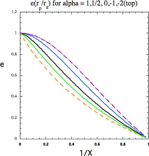
|$\frac{X^k-1}{X^k+1}=e$|. We plot
e as a function of
X for power laws with relevant values of α in Fig.
1.
Figure 1.
Our eccentricity e arises from the equation of the orbit. For power-law potentials, it is plotted as a function of the ratio rp/ra = 1/X for relevant values of α = 1, 1/2, 0, −1, −2 (top).
We have chosen our quadratic
sq(
u) so that it fits well at the ends, but in general a quadratic that fits at the ends with the right gradients there, will not fit so well in the middle. However, we now choose a constant
|$W={\textstyle {\frac{1}{2} }}W_0$| that corrects this,
|${\textstyle {\frac{1}{2} }}e^2 W_0=\sqrt{s_{\rm q}(\bar{u})/s(\bar{u})}-1$|. This constant
W approximation is often so good that further approximation is unnecessary. However, we give a full perturbation theory to all orders in Section 4. Performing the integration in equation (2.13), multiplying by
m and choosing the zero-point of both ϕ and η at the same pericentre, we find
The secular terms which contribute to
m are our main concern, as errors there would cause a gradual drift away in azimuth ϕ between the approximate orbit and the true one. This is seen in Fig.
2. By contrast, the periodic terms such as the sin (2η) term above cause only minor changes in the orbital shape that neither accumulate nor affect
rp,
ra, nor their orientation. If then that term is neglected and we return to our substitution (2.11) and write
|$\bar{u}=l^{-k}$|, the orbit is given by equation (1.1), i.e.
If the small shape changes are retained to first order in their amplitude, we get instead
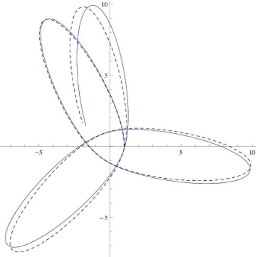
Figure 2.
A computed orbit (full line) and an approximating analytic orbit (dashed) calculated without the perturbation theory. The potential is logarithmic (α → 0) and the axis ratio X = 10 which gives k = 1.4168, e = 0.9262, m0 = 1.5208, m = 1.533. The perturbation theory up to W2 gives 1.544; the best fit is m = 1.542. With that m, the orbit fits the simple form (1.1).
We plot
k as a function of
X for various values of α in Fig.
3(a). Given that our primary variables are
rp,
ra, this determines
k in terms of them and the α that specifies the form of potential. Since both
k and
e occur in the orbital equation, it might seem more natural to plot
k(
e) as in Fig.
3(b) but the definition of
e involves
k so Fig.
3(b) can hardly be used to define
k, rather it is used to tell what values of
e are associated with a given
k(
X).
k is only weakly dependent on eccentricity which is mainly dependent on
X up to
e = 0.9 or even 0.95 but thereafter
k can change by as much as 25 per cent!
k is exactly constant for all
X in the three cases α = 4, 1, −2 with values 0, 1, 2, respectively. These correspond to the inverse fifth power force and the Newtonian and harmonic cases. Attractive power laws with α ≥ 2 give orbits that spiral into the origin. However, as shown in Appendix B, when
k is constant, we may add inverse cubic forces without changing
k. A repulsive
r−5 force coupled with an attractive
r−3 force gives orbits that have both pericentres and apocentres so both
k and
e are defined for them even though α > 2. Such orbits are exactly solvable in terms of elliptic functions. Inverse fifth power forces were discussed by Newton in Principia. He showed that a circle through the centre of attraction was a possible orbit and that this force law was self-dual under the transformation that took orbits in the inverse square law into harmonic orbits. (See Chandrasekhar
1995). Maxwell (
1867) used inverse fifth power repulsions between molecules in his work on the viscosity of gases. For the ψ = −
V2ln
r potential,
k is close to 4/3 for most eccentricities but above
e = 0.95 it increases rapidly to its asymptotic value of 2 for
X large.
LBJ's setting
k = 2 for all orbits was not a good choice! For power laws, equation (2.09) gives
m0 → 2 − α, 2 > α ≥ 0 as
X → ∞ and
|$m_0\rightarrow \sqrt{2-\alpha }, \alpha < 2$| as
X → 1. For all
X,
where,
m0 is plotted in Fig.
4 and the constant
W0 which corrects it to
m via equation (2.14) is plotted in Fig.
5. For the orbit of Fig.
2, α → 0,
X = 10,
k = 1.416 82,
e = 0.92623,
m0 = 1.520 88,
W0 = −0.037 34 so
m = 1.5332. A slow azimuthal drift is evident showing that the perturbation theory of Section
3 is necessary for its correction. The lowest order correction using
W2 gives
m = 1.544 while the best fit to the computed orbit is
m = 1.542. For those who prefer an empirical quick fix to such extra calculation, we have found that setting
m =
mc(1 + 6(|
mc −
m0|/
mc)
(3/2) with
|$m_c=m_0/(1+\textstyle {\frac{1}{4}} e^2W_0)$| works still better. Here, it gives
m = 1.5428 and it also works well for the isochrone orbits. We emphasize that we have chosen to illustrate an orbit with a strong eccentricity that lies in the region where the correction of
m0 to
m is significant (see Fig.
4) and in the logarithmic potential which is the most difficult of the power laws. For less eccentric orbits, the perturbation theory is not needed so the values of
k,
m0,
W0 and hence
m displayed graphically below are all that is needed for a good description.
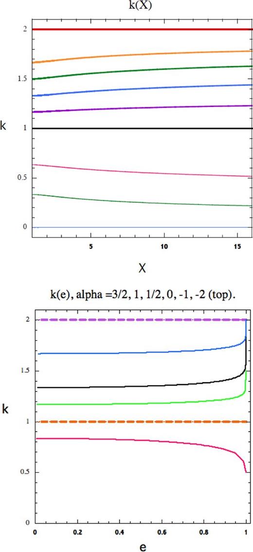
Figure 3.
(a) For power-law potentials ψ = Ar−α, we plot the power k to which 1/r is raised in the equation for the orbit. From bottom α = 4, 3, 2.1, 1, 1/2, 0.01, −1/2, −1, −2 (top). (b) k(e) for α = 1.5, 1, 1/2, 0, −1, −2 (top). k depends only weakly on X or e; except near e = 1.
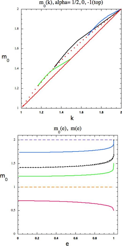
Figure 4.
The angle between apocentres is 2π/m. Above: m0(k) for α = 1/2, 0, −1. Dots and line show the relationships for e = 0, 1. Below: m0(e) for the power potentials α = 3/2, 1, 1/2, 0, −1, −2 (top). For α → 0, we overplot |$m=m_0/(1+\textstyle {\frac{1}{4}\!} e^2W_0)$| as squares. It differs little from the underlying m0 line.
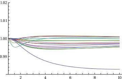
Figure 5.
(a) The Wobble constant W0 gives the small change, |$m =m_0/(1+ {\frac{1}{4}} e^2W_0).$| These changes maximize at 1.3 per cent. Curve order is |$\alpha =0,1/2,-1,(1\; \& \; -2)$| (top). (b) The second wobble constant w0 gives small changes to the radial period. |$T_{\rm r}=T_{\rm r}|_0 [1+\textstyle {\frac{1}{4}}w_0e^2(1-e^2\nu (\nu -1))].$| Here, the curve order has altered |$\alpha =-1,0,1/2,(1\; \& \; -2)$|(top).
2.2 Orbital periods
The time from pericentric passage to a given point at radius
r on the orbit is
The presence of the
u2/k term in the denominator shows that this integral more strongly emphasizes small
u than the integration of equation (2.18). If we look to Kepler's case for guidance, we find that to determine time he uses neither η nor ϕ but his eccentric anomaly χ. This is introduced if in his case we write not
|$u/\bar{u}=l/r=1+e\cos \eta$| but rather
r/
a = 1 −
e cos χ and use χ not η for the integration. This raises a general point concerning integrals involving quadratic surds such as
|$\sqrt{s_{\rm q}(u)}$|. One may write
|$U=u^{-1}=r^k; U_{{\rm a},{\rm p}}=u^{-1}_{{\rm a},{\rm p}}$|. Then,
so writing
|$U/\bar{U}=1-e\cos \chi , \bar{U}={\textstyle {\frac{1}{2} }\!} (r_{\rm a}^k+r_{\rm p}^k)$| and simplifying we have
where ν + 1 = 2/
k. Thus, ν = 1 for Kepler orbits and zero for the central harmonic oscillator. This conversion to χ has eliminated the small denominator that occurs in equation (2.19) for eccentricities near one. Formerly, we thought of
w as a function of
u but now it becomes useful to consider it as a function of χ. It still has to vanish at the end points and it is still symmetrical about pericentre χ = 0 so the zero-order term involves a second constant
w0 and
w is approximated by
|$w={\textstyle {\frac{1}{2} }}e^2w_0\sin ^2\chi$|. We evaluate this term by setting
|${\textstyle {\frac{1}{2} }} e^2 w_0=\sqrt{s_{\rm q}(u^*)/s(u^*)} -1; u^*=1/\bar{U}=2/(r_{\rm a}^k+r_{\rm p}^k)$| cf. equation (2.13). It is this difference in the point of evaluation that is important at high eccentricities. The relationship of η to χ is found by multiplying the expression for
|$U/\overline{U}$| above by equation (2.11) for
u,
This is the same relationship as Kepler found but now for general orbits. The indefinite integral in equation (2.20) is not tractable (but see next section) except for ν = 0, 1; however, the complete integral for the radial period from one apocentre to the next gives a Legendre function, which reduces to simple functions in the interesting range of ν. See Fig.
6.
Setting
|$z=1/(\sqrt{1-e^2})$| for the Legendre functions and taking
|$w={\textstyle {\frac{1}{2} }}e^2w_0\sin ^2\chi$| with
w0 constant as above
For
e ≤ 1,
w0 ≤ 0.1, the final
|$P^2_\nu /P_\nu$| term never contributes more than one part in 300 nevertheless that can be significant as errors in period build up over time. A sufficient approximation when this small term is needed is given by
|$P_\nu ^2/P_\nu =-\nu (\nu -1)(1-z)/(1+z)$|. In Appendix A, we show that
Fν(
z) =
zν/
Pν(
z) is never far from unity and is well approximated to within 0.5 per cent by
where for κ only the major correction term has been included. When the range is extended to −0.2 < ν < 1.8, the accuracy while less good is better than 2 per cent. In the range −0.2 ≤ ν < 1.4
F never differs from unity by more than 10.5 per cent. Notice that for all
z,
F0 = 1 =
F1 and that ν = 0, 1 correspond to the harmonic and Keplerian cases, respectively. Except in those cases there is not normally an exact circumferential period but, since ϕ increases by 2π/
m in time
Tr, the mean circumferential period is
mTr. Figs
7 and
8 show two orbits in the isochrone potential which is not self-similar together with the approximate orbits with the first-order perturbation theory. We have chosen orbits that span the region where the potential has a changing power-law dependence. At higher eccentricities, perturbation theory becomes increasingly necessary and more terms become needed in the perturbation series. Fig.
9 compares the radial period with the exact period for a sequence of orbits in the Isochrone with
rp = 0.3
b fixed and various
ra up to 33.3
b. The program used can have any potential as input but the isochrone has the advantage that exact values of
m and
Tr can be calculated analytically which removes the possibility of errors arising from the orbit integration. For those who prefer an empirical quick fix, the formula given earlier
m =
mc[1 + 6(|
mc −
m0|/
m0)
(3/2)] gives
m to better than 0.07 per cent throughout the sampled range
X ≤ 100/3
e ≤ 0.9828. The errors in
Tr without the perturbation theory are 0.35 per cent at
X = 6,
e = 0.8961, but reach 1.25 per cent at
X = 20,
e = 0.9712. With the perturbation theory, the errors reduce to 0.03 per cent
X = 6 and 0.14 per cent
X = 20. The empirical quick fix formula
Tr =
Tc[1 − (|
Tc −
T0|/
Tc)
(7/4)/0.43], where
Tc is the value without the perturbation theory, gives errors less than 0.05 per cent,
X ≤ 20 rising to 0.14 per cent,
X = 100/3 without the bother of perturbation theory.
Figure 6.
The expression z−νPν(z)Fν(z), which gives the ratio of the exact Legendre expression to our 1/F approximation to it, is plotted as a function of |$z=1/\sqrt{1-e^2}$|. Notice the scale is from 98 per cent to 1.02. The curves are for −0.2 ≤ ν ≤ 1.4. All curves asymptote to one including the deviant curve which is for ν = −0.2. The ν = −0.1 curve is among the others.
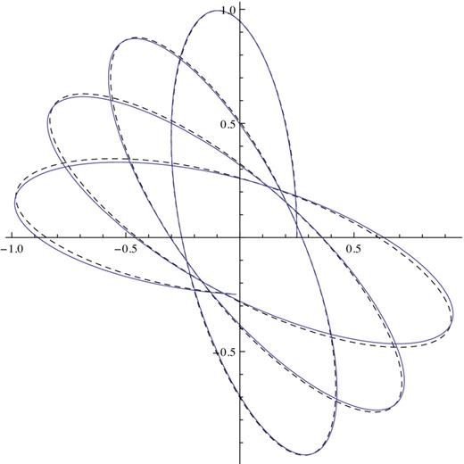
Figure 7.
The approximate orbit (represented by a dashed line) in the isochrone |$\psi =GM/(b+\sqrt{r^2+b^2}$| with ra = 1.2b, rp = 0.3b calculated with the first-order perturbation theory is compared with the computed orbit. The 0.13 per cent difference of the approximate m from the true one is visible after four radial periods.
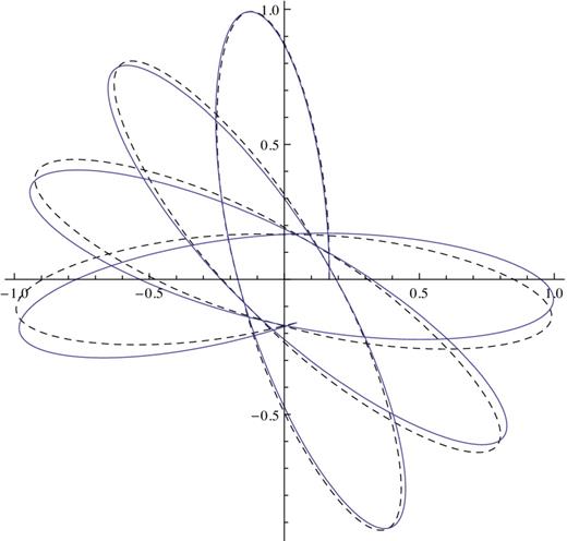
Figure 8.
The approximate orbit (represented by a dashed line) in the isochrone with ra = 1.8b, rp = 0.3b calculated with the first order perturbation theory is compared with the computed orbit. The 0.35 per cent difference of the approximate m from the true one is visible after two radial periods. More Gaussian quadrature points are needed to correct this.
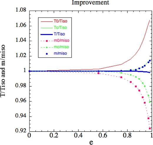
Figure 9.
We show Tr0/Tiso and m0/miso where ‘iso’ denotes exact values for the isochrone together with the improvements (suffix c) generated by using w0 (and W0) in the main theory and finally plotting T/Tiso and m/miso for the first-order perturbation theory that uses w2 (and W2). The orbits all have rp = 0.3b and various ra. For e < 0.8, perturbation theory is hardly needed.
3 ADIABATIC INVARIANTS, ANGLE AND ACTION VARIABLES
The exact expression for the radial action is
Note that the integral is dimensionless and again the
u2 in the denominator emphasises contributions at small
u. It is again appropriate to use
|$U=\bar{U}(1-e\cos \chi )$| rather than
u and convert to an integral over χ. It is also sensible to define a different wobble function,
|$\tilde{w}$| related to our former one by
|$1-\tilde{w}=1/(1+w)$|. If
w is so small that its square can be neglected, then these functions are the same but otherwise they are somewhat different. As the integrand is not symmetrical about χ = π/2, we take the first two terms
|$\tilde{w}=e^2\sin ^2\chi [{\textstyle {\frac{1}{2} }}\tilde{w}_0+\tilde{w_1}\cos \chi ]$| with
|$\tilde{w}_0$| and
|$\tilde{w}_1$| evaluated from
|$e^2 \tilde{w}_0=2[\sqrt{\frac{s(u^*_-)}{s_{\rm q}(u^*_-)}}+\sqrt{\frac{s(u^*_+)}{s_{\rm q}(u^*_+)}}-2], e^2 \tilde{w}_1=\sqrt{8}[\sqrt{\frac{s(u^*_-)}{s_{\rm q}(u^*_-)}}-\sqrt{\frac{s(u^*_+)}{s_{\rm q}(u^*_+)}}]$|, where
|$u^*_-=\frac{u^*}{(1-e/\sqrt{2})},\quad u^*_+=\frac{u^*}{(1+e/\sqrt{2})}$|.
The integrals
|${\cal I}_n=\frac{1}{2\pi }\int _0^{2\pi }\frac{e^{2n}{\rm sin}^{2n}\chi {\rm d}\chi }{(1-e\cos \chi )}$| give
If
m0 is set equal to
qk, the term in
|${\cal I}_1$| agrees with the result given in
LBJ. The correction terms in
|$\tilde{w}_0,\tilde{w}_1$| were not applied there.
Equation (3.27) gives an accurate value of Jr but we often want its derivatives with respect to ε or h. These we have already since ∂Jr/∂ε = Tr/(2π) and ∂Jr/∂h = −1/m.
Thus, we do not need to eliminate k, m0, e in Jr in favour of ε, h. However, if Jr(ε, h) is known either by Williams's method (see below) or e.g. for the isochrone then we can check these results.
3.1 Timing, Hamilton's action, and a generalized Kepler equation
If
|$H({\boldsymbol p},r)$| is the Hamiltonian in the plane of motion, the Hamilton–Jacobi equation
H(∂
S/∂
r, ∂
S/∂ϕ,
r) = ε is an equation for Hamilton's action
S.
It separates in the form
S =
Sr +
Sϕ, where
Here, I have inserted ε,
h as the separation constants. The radial action is
Jr = (2π)
− 1∮
pr d
r. The angle variables are
|$w_\phi =\mathrm{\partial} S/\mathrm{\partial} J_\phi =\phi +(\mathrm{\partial} S_r/\mathrm{\partial} h)_{J_r}$| and
wr = ∂
S/∂
Jr = (∂
S/∂ε)/∂(
Jr/∂ε) = 2π∂
S/∂ε/
Tr. These give the phases of the motion in ϕ and
r which advance uniformly in time.
When we want the time to a given point in the orbit, we differentiate Hamilton's action. 2π times the incomplete integrals for
Jr give us the radial part,
Sr(
r, ε,
h), of Hamilton's Principal Action from which the time to a given point in the orbit can be deduced. Because this involves differentiating an approximate expression, it is intrinsically less accurate than our direct evaluation of the radial period given above. For this reason, we only use the following calculation to evaluate the fraction of the radial period taken to a given point and multiply that fraction by our more accurate period. Evaluating the incomplete integral in equation (3.26) in terms of the integrals
|$I_n(\chi )=\int _0^\chi [e^{2n}\sin ^{2n}(\chi )/(1-e\cos \chi )]\,{\rm d}\chi$|It is easy see that the
In(2π) reduce to
|$2\pi {\cal I}_n$| as defined earlier. Since
|$S_r=\int _{r_{\rm p}}^r[\dot{r}]{\rm d}r=\int _{r_{\rm p}}^r \sqrt{2 \varepsilon +2\psi -h^2/r^2} {\rm d}r$|, we see that
|$\mathrm{\partial} S_r(\varepsilon ,h,r)/\mathrm{\partial} \varepsilon =\int _{r_{\rm p}}^r[1/\dot{r}]{\rm d}r=t$| so differentiation gives us the time to a given point. However, this differentiation is awkward because we have
Sr expressed in terms of different variables most of which depend on ε.
For orbits in power-law potentials or close to those, a good but very different method that eliminates this difficulty is described by Williams, Evans & Bowden (2014).
However, persisting with our general case and differentiating only the terms that vary significantly, we find for ∂
Sr/∂ε
To these, we can add on the right the smaller terms now omitting
|$\tilde{w}_1$| terms
whenever those are significant. Using the partial derivatives of
e and χ evaluated in Appendix B, equation (3.31) becomes
where the small terms in ∂ln
k/∂ε have been omitted from equation (3.32). Thus, the fraction of the total radial period is (2π)
− 1[χ − (
V2/
V1)
esin χ] and the time is
where
Tr is given by equation (2.23). Notice that for Kepler
V1 = 1 =
V2 so equation (3.33) becomes Kepler's equation while for the central harmonic oscillator
V1 = 1 −
e2,
V2 = 0, giving χ ∝
t. For both those cases, the small terms are identically zero. Thus, equation (3.33) is the generalization of Kepler's equation. Furthermore, for 1 ≤
k < 2,
V2/
V1 → 1 as
e → 1 so equation (3.33) then reduces to Kepler's equation.
Not uncommonly, one wants χ(t) rather than t(χ) as given by Kepler's equation. The problem of inverting Kepler's equation analytically has intrigued mathematicians and astronomers down the centuries. My recent analysis (Lynden-Bell 2015), designed for the general orbits above, is good to one part in ten thousand before any iterative procedure is used.
In Henon's isochrone potential |$\psi = GM/[b+\sqrt{r^2+b^2}]$|, the radial period is a function of energy but independent of angular momentum so ∂2Jr/∂ε∂h = 0, which implies that the angle between successive apocentres, 2π/m = −2π∂Jr/∂h is a function of angular momentum but not of energy. As many galactic potentials are not far from isochronal, it is often the case that m is only weakly dependent of energy and that Tr is only weakly dependent on angular momentum.
4 PERTURBATION THEORY
We show here how the theory can be developed to all orders so that the orbits can be found to any desired accuracy. In equation (2.6), we wrote
s(
u) =
sq(
u)/[1 +
w(
u)]
2 and we later showed that
w(
u) could be written as
|$s_{\rm q}(u)/[1+(u_{\rm p}-u)(u-u_{\rm a})\bar{u}^{-2}W(u)]^2$|. We now Fourier analyse the function
W(
u) over the range
ua to
up as a function of cos (η) writing
For general potentials, it may not be possible to perform the integration needed to find the Fourier coefficients
Wn but Gaussian integration allows us to evaluate them. If we want the series up to cos (
Nη), we evaluate the function on the left at the zeros of cos [(
N + 1)η] and from those values we find the
N coefficients. In particular, if we wish to stop at cos (2η), then we have to evaluate the
W[η] of equation (4.34) at η = π/6, π/2, 5π/6, the zeroes of cos (3η) and the coefficients are for
W[η] re-expressed as a function of η
Our earlier evaluation of
W0 is this same process applied to equation (4.34) when all
Wi,
i > 0 are neglected. However, when those higher terms are included, the evaluation as above supercedes the earlier one. In place of equation (2.15), the relationship of ϕ to η is now given by
m0ϕ = η + ∫
e2sin
2η
W[η]dη and from equation (4.34), the integration is simple with the secular term on the right being
|$\eta [1+\textstyle {\frac{1}{4}} e^2(W_0-W_2)]$|. Thus, none of the higher order terms contribute to the angle between apsides and the value of
m, which is exact in so far as the
W0 and
W2 are exact, is given by
When applied to the orbit of Fig.
2, we find
W[π/2] = −0.019,
W[π/6] = −0.008,
W[5π/6] = −0.129. These give
W0 −
W2 = −0.071,
m = 1.544 which slightly overshoots the best-fitting value
m = 1.542. We note that this is probably due to the relatively large value of
W[5π/6]; however, we felt going to more terms in the Gaussian quadrature to find
W0 −
W2 would add only tedium. Defining the new
|$\tilde{W_i}=(m/m_0)W_i$| and treating the
Wi as first-order quantities, we find that the orbital equation becomes
For the perturbed period, we expand in terms of χ rather than η because fewer terms then give the main contribution. Expanding
w/(
e2 sin
2χ) as a Fourier series in cos (
nχ), we have
|$w=e^2\sin ^2\chi ({\textstyle {\frac{1}{2} }}w_0+\sum _1^\infty w_n\cos (n\chi )=\textstyle {\frac{1}{4}} e^2[(w_0-w2)+\sum _1^\infty (-w_{n-2}+2w_n-w_{n+2})\cos (n\chi )]$| where
wn = 0 when
n < 0. Again the coefficients
wn can be evaluated analogously to equation (3.35) but now at the places where cos [(
N + 1)χ] = 0
where the
|$P_\nu ^n$| are all functions of
|$z=1/\sqrt{1-e^2}$|. These can be replaced by simple functions by following the work in Appendix A which shows that in the range of interest
expressions for the
|$P^n_\nu$| are also given there.
To get
Jr, we have to expand the
|$[1-\tilde{w}(u)]$| above (equation 3.26) in the form
|$\tilde{w}=e^2\sin ^2\chi [{\textstyle {\frac{1}{2} }} \tilde{w}_0+\sum _1^\infty (\tilde{w_n}\cos (n\chi )]$|, where
|$\tilde{w}_n=0$| for
n < 0.
Expressions for the
Kn can be found in Gradsteyn & Ryzbik (
2000).
I thank Curtis Struck for sending me his preprints prior to publication.
REFERENCES
. ,
Newton's Principia for the Common Reader
,
1995
Oxford
Oxford Univ. Press
, . ,
Tables of Integrals 6th edn (Formula 3.616,7)
,
2000
San Diego, CA
Academic Press
. ,
MNRAS
,
2010
, vol.
402
pg.
1937
. , , . ,
Galaxies and their Masks
,
2012
New York
Springer
pg.
233
. ,
MNRAS
,
2015
, vol.
447
pg.
363
, . ,
MNRAS
,
2008
, vol.
386
pg.
245
. ,
Phil. Trans. R. Soc.
,
1867
, vol.
157
pg.
49
. ,
AJ
,
2006
, vol.
131
pg.
1347
, . ,
MNRAS
,
2009
, vol.
389
pg.
1069
, , . ,
MNRAS
,
2011
, vol.
414
pg.
2498
, . ,
Modern Analysis, 4th edn. Cambridge Univ. Press, Cambridge
,
1927
, , . ,
MNRAS
,
2014
, vol.
442
pg.
1405
APPENDIX A: Approximating the Legendre function for periods
We now give the reasoning that leads to the formulae for
Tr,
Fν quoted above. Laplace's integral defines the Legendre function
|$P_\nu (z)=P_\nu ^0(z)$| and the associated
so the functions needed in equation (2.23) are
z− νPν and
|$z^{-\nu}P^2_\nu$| with
|$z=1/\sqrt{1-e^2}, \nu =(2/k)-1$|. However, though it may be reassuring to be told that we are dealing with named functions, that are not always a great help in knowing their behaviour and evaluating them. The formula (Whittaker & Watson
1927)
tells us that we need only to evaluate the Legendre functions themselves and the associated ones can then be derived from them. Kepler's orbits in the 1/
r potential have
k = 1 and therefore ν = 2/
k − 1 = 1. Simple harmonic orbits in the very different
r2 potential have
k = 2, ν = 0. Insofar as these correspond to the limits of a perfectly concentrated mass point and a uniform density system, we may feel that they give natural limits to the values of
k that we shall encounter. However, gravity is not the only force field so we shall extend the range of our interest to −0.2 < ν < 1.6 corresponding to 2.5 >
k > 0.77. The asymptotic form for
Pν at large
z is proportional to
zν with
The expression on the right is unity at ν = 1 and at ν = 0 and only varies by 10 per cent in between. After a little experimentation, we found it was well fitted by the expression
This formula gives better than 0.1 per cent accuracy in the range indicated and the accuracy only falls to 0.5 per cent when the range is extended to −0.2 < ν < 1.7. The gamma function diverges at ν = −0.5 so the accuracy falls away rapidly for ν < −0.2.
However, we are not merely interested in the asymptotic values but in all values of
z ≥ 1. At the lower limit,
z = 1 corresponding to
e = 0,
z−νPν = 1 for all values of ν. This is also true for all
z at ν = 0 and 1 so our function is 1 or nearly 1 on all sides of a box. This suggests that it may not be far from one even within the box and even a little way outside the box to smaller and larger values of ν. To get enlightenment as to what form our approximation should take, we first considered the case when ν is small. Then
|$z^{-\nu}P_{\nu}(z)=\int_{-\pi}^{\pi} \ln(1+e\cos\chi)d\chi$| is evaluated in tables so for ν small
|$F_{\nu}(z)=1-\nu\, \ln [{\textstyle {\frac{1}{2} }}(1+z^{-1})]$| asymptotically this gives 1 + ν ln (2). From this, we understood that the factor 11/4 = 2.75 in equation (A4) should really be 4 ln 2 = 2.7726. Since this only corrects the correction to one, it is no surprise that replacing the 11/4 by 4ln 2 fits just as well and of course more accurately for ν small. Expanding equation (A1) using the binomial theorem and comparison to our formula for the asymptotic form led us to the empirical formula
Within that range of ν, the error is less than 0.5 per cent for all
z ≥ 1.The error is greater with a maximum of 2 per cent if we extend the range to ν = −0.2. This may be seen from Fig.
6 where the ratio of the full Legendre-function-expression to our approximation is plotted for 16 values of ν and the relevant range of
z. All the curves asymptote to unity at large
z outside the range illustrated. Take heed of the much expanded scale on the left under which a 2 per cent deviation looks large. The one deviating curve is that for ν = −0.2. The ν = −0.1 curve is among the others. It is not good practice to differentiate an approximation especially if the whole is almost constant as that constant will not contribute to the differential which may have a much larger percentage error. To get the associated Legendre functions from the Legendre functions via equation (A1), we have to do that. But the Legendre functions that concern us are not constant but vary like
zν and when ν is small they give the exact result; furthermore they only occur as coefficients of the correction terms involving
w; a somewhat larger error can be tolerated in the coefficient of a small term. Finally to get
|$P_\nu ^2(z)$|, we need only differentiate once because by Legendre's equation
|$P_\nu ^2=(z^2-1){\rm d}^2P_\nu /{\rm d}z^2=[\nu (\nu -1)-2{\rm d}\ln (z^{-\nu }P_\nu )/{\rm d}\ln z]P_\nu (z)$|. We can thus use equations (A2) and (A5) for
|$P_\nu ^1\; \& \; P_\nu ^2$|.
APPENDIX B: PARTIAL DERIVATIVES. WHEN ARE k, m CONSTANT?
B1 Evaluation of |$\partial e/\partial \varepsilon$|
Since
k does not vary much, the derivatives of ln
k are often negligible. Also since
m,
m0 are mainly dependent on
h, their derivatives at constant
h are likewise small. Differentiating our definition of eccentricity (equation 2.13)
Differentiating equation (1.2) at constant
h and using equation (2.18)
Eliminating
rp,
ra in favour of
l,
e, we find the partial derivative of
e2.
where the final term is almost always small. We checked this expression for Keplerian and simple harmonic orbits.
B2 The partial derivative of χ
Differentiating logarithmically
|$r^k={\textstyle {\frac{1}{2} }}(r_{\rm a}^k+r_{\rm p}^k)(1-e\cos \chi )$| at constant
h and
r, we find after rearrangement
After evaluating the final two terms, this becomes
where the term
|$+\frac{\mathrm{\partial} \ln k}{\mathrm{\partial} \varepsilon }\ln [\frac{(1-e\cos \chi )}{\sqrt{1-e^2}}(\frac{1-e}{1+e})^{e/2}]$| should be added on the right when it is not negligible.
B3 The variation of k, a new property of r−5 forces
We have seen that
k = 1 for Kepler's orbits and
k = 2 for the central harmonic oscillator. Are there any other central potentials for which
k is exactly constant? To investigate this, we write
y =
r−2 so that
r3ψ
′ = −2 dψ/d
y and from equation (1.3)
h2 = 2Δψ/Δ
y, where Δ stands for the difference between pericentric and apocentric values. Then following equation (2.8)
Expanding to second order in
ya −
yp and no further, we find
So for
k to be constant at small radial amplitudes, we must have
where
K is constant.
Integrating this differential equation for ψ and omitting the irrelevant zero-point constant
Returning to equation (B6), it is evident that the
B term does not contribute to dψ/d
y − Δψ/Δ
z even at finite amplitude so it can be added to a potential which gives constant
k without changing
k. This was known to Newton and used in Principia to demonstrate the exactness of the inverse square from the lack of precession of the major axes of the planets. Evidently, generalized power laws with such
B terms added are the only candidates for giving constant
k but we must now consider them at ALL Δ
y not just small ones. We must have
where
x =
ya/
yp.
For K > 0, the terms in the higher powers come earlier in both numerator and denominator so on division by xK+1 we need K/xK+1 = 1/x2 = 1/(KxK + 1) so K = 1, k = 0 This gives the potential |$\psi ={\textstyle {\frac{1}{2} }}A z^2+B z={\textstyle {\frac{1}{2} }}Ar^{-4}+Br^{-2}$|. To get an orbit with two turning points, we need an attractive potential Br−2 with B positive and a repulsive |${\textstyle {\frac{1}{2} }}Ar^{-4}$| potential with A negative. It is at first off-putting that this case has k = 0 but when we use u = ln r, we find that indeed s′(up) = −s′(ua) as desired.
K = 0 is one of our special cases discussed later.
For 0 > K > −1, the leading term in the numerator is still −KxK + 1 but the next is now −1. The leading term in the denominator is now (K + 1)x and the next is −xK + 1 so we need −KxK/(K + 1) = 1/xK + 1 = −(K + 1)xK/K which is true only for |$K=-{\textstyle {\frac{1}{2} }}, k=1.$| This is Kepler's case, with Newton's generalization to include the B term.
K = −1 is the other special case discussed presently.
For K < −1, the leading terms in the numerator of equation (B11) are −1 and then −KxK + 1 while those in the denominator are (K + 1)x and then −K so we need −x−1/(K + 1) = xK + 1 = −(K + 1)/x. This holds only for K = −2, k = 2. This is the central harmonic oscillator with the possible addition of the inverse cubic force. |$\psi ={\textstyle {\frac{1}{2} }}Ar^2+B r^{-2}$|.
This leaves only the special cases K = 0, −1; however, when we inspect the ratio which is the central member of equation (B11) we find mixtures of y and ln y terms in both numerator and denominator that cannot cancel to leave a power of x. Thus, neither special case leads to a constant k system of orbits. In summary, we have added only the r−4 case and the B terms to those already discussed.
We now turn to equation (2.9) for the evaluation of ∂
k/∂ε in general
Hence, using equation (B2)
B4 Partial derivative of m0
In Kepler's elliptical orbits, the angle Φ subtended at the centre by successive apocentres is 2π. For a central harmonic oscillator, it is π. In general, the angle is 2π/
m but this varies from orbit to orbit. Henon discovered his isochrone from the condition that the radial period should depend on the energy of the orbit but be independent of its angular momentum. Thus for the isochrone, ∂
Jr/∂ε is independent of
h. But that same condition implies that ∂
Jr/∂
h = Φ/(2π) must be independent of ε. However, for the isochrone this is NOT independent of
h so we deduce that there are no potentials other than the above ones for which all orbits have the same precession angle Φ. However, when the potential is not far from isochronal we may expect that
m is mainly a function of angular momentum and only weakly dependent on energy. From differentiating equation (2.11) logarithmically
© 2015 The Author Published by Oxford University Press on behalf of the Royal Astronomical Society


![(a) The Wobble constant W0 gives the small change, $m =m_0/(1+ {\frac{1}{4}} e^2W_0).$ These changes maximize at 1.3 per cent. Curve order is $\alpha =0,1/2,-1,(1\; \& \; -2)$ (top). (b) The second wobble constant w0 gives small changes to the radial period. $T_{\rm r}=T_{\rm r}|_0 [1+\textstyle {\frac{1}{4}}w_0e^2(1-e^2\nu (\nu -1))].$ Here, the curve order has altered $\alpha =-1,0,1/2,(1\; \& \; -2)$(top).](https://oup.silverchair-cdn.com/oup/backfile/Content_public/Journal/mnras/447/2/10.1093_mnras_stu2485/2/m_stu2485fig5.jpeg?Expires=1716396871&Signature=ryArlKMZKwSEFkdGmYjvNBJrjmvSHhXE3iu3zaFt41cqGR9k-I68if01383cZCamXvFDFhYILwK9iOe-w8B9UczwberIs4eSWSTSnTTqe76yN2PmHq7ngvJGigxfXJpK-6b~SK4Sr1xWge4k8ZDr1FYaGxUwnXDj~BmMGf7sBCw~yAb4DxyfIwqGvvIkV4wFaIQw5rH~vgKaCK59tXmyRCNB8LVFtW4jBIcnYbL2uOWwjRunqK6stftuwRT79rZHrMZFa-VOhlqZOOBmaQSUP~HKmKY9SvaIvFujJkUoCMSB4QGFs3EGa1BQ0PHFYhA2-uVWzFGVB0pmN561m5CC~g__&Key-Pair-Id=APKAIE5G5CRDK6RD3PGA)
