


Abstract
Using the 2MASS near-infrared photometry and high-signal-to-noise H i 21-cm data from the Arecibo, Green Bank, Nancay, and Parkes telescopes, we calculate the redshift-independent distances and peculiar velocities of 2018 bright inclined spiral galaxies over the whole sky. This project is part of the 2MASS Tully-Fisher survey (2MTF), aiming to map the galaxy peculiar velocity field within 100 h−1 Mpc, with an all-sky coverage apart from Galactic latitudes |b| < 5°. A χ2 minimization method was adopted to analyse the Tully–Fisher peculiar velocity field in J, H, and K bands, using a Gaussian filter. We combine information from the three wavebands, to provide bulk flow measurements of 310.9 ± 33.9 , 280.8 ± 25.0, and 292.3 ± 27.8 km s−1 at depths of 20, 30, and 40 h−1 Mpc, respectively. Each of these bulk flow vectors points in a direction similar to those found by previous measurements. At each of the three depths, the bulk flow magnitude is consistent with predictions made by the Λ cold dark matter (ΛCDM) model at the 1σ level. The maximum likelihood and minimum variance method were also used to analyse the 2MTF samples, giving similar results.
INTRODUCTION
Galaxy redshifts exhibit deviations from Hubble's law known as ‘peculiar velocities’, which are induced by the gravitational attraction of all surrounding matter. Peculiar velocities thus provide a means to trace the overall matter density field and detect all gravitating matter (both visible and dark). Peculiar velocities can be measured using redshift-independent distance indicators. Several such indicators have been used, including Type Ia SNe (Phillips 1993), the Tully–Fisher relation (TF; Tully & Fisher 1977) and the Fundamental Plane relation (FP; Djorgovski & Davis 1987; Dressler et al. 1987). The largest peculiar velocity surveys make use of either the FP or TF relations. One limitation of these, and many other, redshift-independent distance indicators, however, is that they rely on optical photometry or spectroscopy. This means that the optical extinction effects of our Galaxy limit the sky coverage of such surveys in the so-called Zone of Avoidance (ZoA).
The 2MASS Tully-Fisher Survey (2MTF; Masters, Springob & Huchra 2008; Hong et al. 2013; Masters et al. 2014) is an all-sky TF survey aiming to measure the redshift-independent distances of nearby bright spiral galaxies. All galaxies in the 2MTF sample were selected from the 2MASS Redshift Survey (2MRS; Huchra et al. 2012), which is an extended redshift survey based on the 2 Micron All-Sky Survey Extended Source Catalog (Jarrett et al. 2000). By using the near-infrared (NIR) photometric data and high-quality 21-cm H i data from the Green Bank Telescope (GBT), Parkes radio telescope, Arecibo telescope, and other archival H i catalogues, 2MTF provides sky coverage down to Galactic latitude |b| = 5°, which significantly reduces the area of the ZoA relative to previous TF surveys.
One parameter of the peculiar velocity field that benefits from the improved sky coverage of 2MTF is the dipole, or ‘bulk flow’. In past measurements of the bulk flow of the local Universe, authors have largely agreed on the direction of the flow, but disagree on its amplitude (Hudson et al. 2004; Feldman, Watkins & Hudson 2010; Dai, Kinney & Stojkovic 2011; Ma, Branchini & Scott 2012; Ma & Scott 2013; Rathaus, Kovetz & Itzhaki 2013; Ma & Pan 2014). Watkins, Feldman & Hudson (2009) analysed a peculiar velocity sample of 4481 galaxies with a ‘Minimum Variance’ (MV) method, within a Gaussian window of radius 50 h−1 Mpc. They found a bulk flow with amplitude 407 ± 81 km s−1, which they claim is inconsistent with the Λ cold dark matter (ΛCDM) model at >98 per cent confidence level.
On the other hand, other studies have shown a bulk flow amplitude agreeing with the ΛCDM model. By estimating the bulk flow of the SFI++ TF sample (Masters et al. 2006; Springob et al. 2007), Nusser & Davis (2011) derived a bulk flow of 333 ± 38 km s−1 at a depth of 40 h−1 Mpc, which is consistent with the ΛCDM model. Turnbull et al. (2012) adopted the bulk flow estimation on a Type Ia SNe sample with 245 peculiar velocity measurements, finding a bulk flow of 249 ± 76 km s−1, which is also consistent with the expectation from ΛCDM.
In this paper, we use 2MTF data to measure the bulk flow in the local Universe. The relatively even sky coverage and uniform source selection criteria make 2MTF a good sample for bulk flow analysis. The data collection is described in Section 2. Section 3 introduces the calculations of TF distances and peculiar velocities. A χ2 minimization method was adopted to analyse the peculiar velocity field, which is presented in Section 4. We compared our measurements with the ΛCDM predictions and previous measurements in Section 5. A summary is provided in Section 6.
Throughout this paper, we adopt a spatially flat cosmology with Ωm = 0.27, |$\Omega _\Lambda = 0.73$|, ns = 0.96 (WMAP-7 yr; Larson et al. 2011). All distances in this paper are calculated and published in units of h−1 Mpc, where the Hubble constant is given by H0 = 100 h km s−1 Mpc−1. The observational results in this paper are independent of the actual value of h, though we compare with a ΛCDM model in Section 5 which assumes the WMAP-7 yr value of h = 0.71.
DATASETS
To build a high-quality peculiar velocity sample, all 2MTF target galaxies are selected from 2MRS using the following criteria: total K magnitudes K < 11.25 mag, cz < 10 000 km s−1, and axis ratio b/a < 0.5. There are ∼6000 galaxies that meet these criteria, but many of them are faint in H i, so observing the entire sample would be very expensive in terms of telescope time. We have combined archival H i data with observations from the Arecibo Legacy Fast ALFA survey (ALFALFA; Giovanelli et al. 2005) and new observations made with the GBT and Parkes radio telescope. The new observations preferentially targeted late-type spirals deemed likely to be H i rich, but the archival data includes all spiral subclasses. Accounting for galaxies eliminated from the sample because of confusion, marginal signal-to-noise ratio (SNR), non-detections, and other problematic cases, as well as cluster galaxies reserved for use in the 2MTF template (Masters et al. 2008), current peculiar velocity sample from 2MTF catalogue contains 2018 galaxies. As shown in Fig. 1, the catalogue provides uniform sky coverage down to Galactic latitude |b| = 5°, which makes it a good sample for bulk flow and large-scale structure analysis.
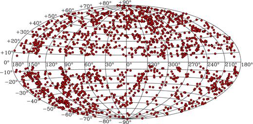
Sky coverage of the 2018 2MTF galaxies, in Galactic coordinates with an Aitoff projection.
We note that the sample of 2018 galaxies discussed here is separate from the 888 cluster galaxies used to fit the template relation for 2MTF in Masters et al. (2008). The relationship between that template sample and the field sample is discussed further in Section 3.1.
Photometric data
All 2MTF photometric data are obtained from the 2MRS catalogue. 2MRS is an all-sky redshift survey based on 2MASS. It provides more than 43 000 redshifts of 2MASS galaxies, with K < 11.75 mag and |b| ≥ 5°. The photometric quantities which are adopted for the TF calculations are the total magnitudes in J, H, and K bands, the 2MASS co-added axis ratio b/a (the axis ratio of J+H+K image at the 3σ isophote; for more details see Jarrett et al. 2000) and the morphological type code T.
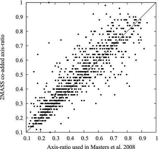
Masters et al. (2008) built the 2MTF TF template using the axis ratio in I band and J band. However, the I-band axis ratio are only available for a small fraction of the 2MTF non-template galaxies. Thus, to make the 2MTF non-template sample more uniform, we chose the 2MASS co-added axis ratio as our preferred data. As shown in Fig. 2, we took the 888 2MTF template galaxies as a comparison sample and compared the 2MASS co-added axis ratio with the axis ratio used in the 2MTF template. A dispersion was found between these two parameters (∼0.096), which we expect will introduce a small scatter into the final TF relation, but no significant bias was detected in this comparison.
Galaxy internal dust extinction and k-correction were done following Masters et al. (2008). The total magnitudes provided by the 2MRS catalogue have already been corrected for Galactic extinction, so no additional such correction was applied here.
H i rotation widths
Archival data
Before making our new H i observations, we collected high-quality H i width measurements from the literature. The primary source of 2MTF archival data is the Cornell H i digital archive (Springob et al. 2005). The Cornell H i digital archive provides about 9000 H i measurements in the local Universe (−200 < cz < 28 000 km s−1) observed by single-dish radio telescopes. When cross-matching this H i data set with the 2MRS catalogue, we include only the galaxies with quality codes suggesting suitability of the measured width for TF studies, G (Good) and F (Fair) in the nomenclature of Springob et al. (2005). (See section 4 of that paper for details.) 1038 well-measured galaxies in this data set which meet the 2MTF selection criteria were taken into the final 2MTF catalogue. The H i widths provided by Springob et al. (2005) were corrected for redshift stretch, instrumental effects and smoothing, we have added the turbulence correction and viewing angle correction to make the corrected widths suitable for the TF calculations.
Besides the Cornell H i digital archive, we also collected H i data from Theureau et al. (1998, 2005, 2007), Mathewson, Ford & Buchhorn (1992) and Nancay observed galaxies in table A.1 of Paturel et al. (2003). The raw observed widths taken from these sources were corrected for the aforementioned observational effects following Hong et al. (2013).
GBT and parkes observations
In addition to the archival H i data, new observations were conducted by the GBT and the Parkes radio telescope between 2006 and 2012.
1193 2MTF target galaxies in the region of δ > −40° were observed by the GBT (Masters et al. 2014) in position-switched mode, with the spectrometer set at nine level sampling with 8192 channels. After smoothing, the final velocity resolution was 5.15 km s−1. The H i line was detected in 727 galaxies, with 483 of them considered good enough to be included into the 2MTF catalogue.
The Parkes radio telescope was used to observe the targets in the declination range δ ≤ −40° (Hong et al. 2013). We observed 305 galaxies which did not already have high-quality H i measurements in the literature and obtained 152 well-detected H i widths (SNR > 5). Beam-switching mode with seven high-efficiency central beams was used in the Parkes observations. The multibeam correlator produced raw spectra with a velocity resolution Δv ∼ 1.6 km s−1, while we measured H i widths and other parameters on the Hanning-smoothed spectra with a velocity resolution of ∼3.3 km s−1.
All newly observed spectra from the GBT and Parkes telescope were measured by the same idl routine awv_fit.pro, which based on the algorithm used by Springob et al. (2005). H i line widths were measured by five different methods (see Hong et al. 2013, section 2.1.2). We chose WF50 as our preferred width algorithm. This fitting method can provide accurate width measurements for low-SNR spectra. It was adopted as the preferred method by the Cornell H i digital archive and the ALFALFA blind H i survey.
ALFALFA data
The GBT observations did not cover the entirety of the sky north of δ = −40°. 7000 deg2 of the northern (high Galactic latitude) sky were observed by the ALFALFA survey. In this region of the sky, we rely on the ALFALFA observations, rather than making our own GBT observations. In this region, ALFALFA is expected to detect more than 30 000 H i sources with H i mass between 106 and 1010.8 M⊙ out to z ∼ 0.06. The ALFALFA data set has not been fully released yet. Haynes et al. (2011) published the α.40 catalogue which covers about 40 per cent of the final ALFALFA sky. However, the ALFALFA team has provided us with an updated catalogue of H i widths, current as of 2013 October. The new catalogue covers about 66 per cent of the ALFALFA sky. From this data base, the 2MTF catalogue obtained 576 H i widths. When the final ALFALFA catalogue is released, we will correspondingly update the 2MTF catalogue, making use of the complete data set.
Data collecting limit of TF sample
The initial 2MTF catalogue includes 2708 galaxies. An additional cutoff was employed to improve the data quality. Only the well-measured galaxies were included in the 2MTF peculiar velocity sample. That is, we include those galaxies with cz ≥ 600 km s−1, relative H i width error |$\epsilon _\mathrm{w}/w_{\mathrm{H\,\small{I}}} \le 10$| per cent and H i spectrum SNR ≥ 5. 141 galaxies in the template sample of Masters et al. (2008) were excluded. The current 2MTF peculiar velocity sample has 2018 galaxies with good enough data quality for the TF distance calculations and further cosmological analysis. The sky coverage and redshift distribution of the 2MTF peculiar velocity sample are plotted in Figs 1 and 3, respectively.
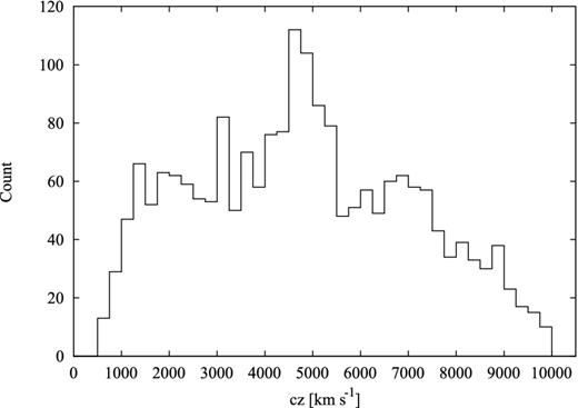
The redshift distribution of the 2MTF sample in the CMB frame.
DERIVATION OF TF DISTANCES AND PECULIAR VELOCITIES
Template relation
Using 888 spiral galaxies in 31 nearby clusters, Masters et al. (2008) built TF template relations in the 2MASS J, H, and K bands, following the approach taken by Masters et al. (2006) for SFI++, which in turn follows the approach of Giovanelli et al. (1997) for SCI. The authors found a dependence of the TF relation on galaxy morphology, with later spirals presenting a steeper slope and a dimmer zero-point on the relation than earlier type spirals. This morphological dependence occurs in all three 2MASS wavebands. The final template relations were corrected to the Sc type in the three bands, as was done for in the I-band relation examined by Masters et al. (2006).
TF distance and peculiar velocity calculations
As shown in Fig. 2, the difference between the two sources of inclination introduces a mean scatter of 0.096, so we adopted a uniform scatter σinc = 0.1 as the inclination error. The inclination uncertainty then introduces errors into the TF distances. For a galaxy with inclination b/a, we calculated the corrected H i width with b/a ± 0.1, and got the corrected widths Whigh and Wlow, respectively. Half of the difference between the two widths, Δwid, inc = 0.5(Whigh − Wlow), was then adopted as the error introduced by the inclination into the H i corrected width. Finally, the error introduced to the TF distances by inclination uncertainty, ϵinc, was calculated using the same approach undertaken to calculate the contribution from the HI width uncertainty, ϵwid.
The TF relations in the three bands are shown in Fig. 4, along with the template relations. We also show the observational errors for both the H i width and NIR magnitudes.
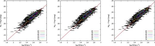
TF relations for 2MTF galaxies in the J, H, and K bands (left to right). The red solid lines are the TF template relations in the three bands. By making a 50 × 50 grid on the TF relation surface log W–M, we counted the number of galaxies falling in every grid point, and took these counts as the number density of the TF plot, which are indicated by the colour contours.
Member galaxies of galaxy groups
We cross-matched the 2MTF galaxies with the group list identified by Crook et al. (2007). 55 galaxy groups have more than one member in the 2MTF sample. We assume all member galaxies in a given group have the same redshift. That is, when doing the calculation in equation (2), all member galaxies in a group are assigned the group redshift czgroup, while the magnitude offset ΔM was still calculated separately for each galaxy.
Malmquist bias correction
The term ‘Malmquist bias’ describes a set of biases originating from the spatial distribution of objects. There are two types of biases that one may consider. Inhomogeneous Malmquist bias arises from local density variations along the line of sight, and is much more pronounced when one is working in real space. This is because, as explained by Strauss & Willick (1995), the large distance errors cause the observer to measure galaxy distances scattered away from overdense regions in real space. In contrast, the much smaller redshift errors mean that this effect is insignificant in redshift space. While some other TF catalogues, such as SFI++, included galaxy distances in real space, the fact that we operate in redshift space means that inhomogeneous Malmquist bias is negligible. However, we must account for the second type of Malmquist bias, homogeneous Malmquist bias.
Homogeneous Malmquist bias comes about as a consequence of the selection effects of the survey, which cause galaxies to be preferentially included or excluded from the survey, depending on their distance. Ideally, the survey selection function is a known analytical function, allowing for a relatively straightforward correction for selection effects. However, galaxy peculiar velocity surveys often have complex selection functions, requiring ad hoc approximations in the application of Malmquist bias corrections (e.g. Springob et al. 2007).
In the case of 2MTF, we used homogeneous criteria in determining which galaxies to observe. As explained in Section 2, all 2MRS galaxies with K < 11.25 mag, cz < 10 000 km s−1, and b/a < 0.5 that also met our morphological selection criteria were targeted for inclusion in the sample. However, many of the targeted galaxies were not included in the final sample, because there was no H i detection, the detection was marginal, or there was some other problem with the spectrum that prevented us from making an accurate TF distance estimate.
We thus adopt the following procedure for correcting for Malmquist bias (explained in more detail by Springob et al., in preparation).
Using the stepwise maximum likelihood method (Efstathiou, Ellis & Peterson 1988), we derive the K-band luminosity function for all galaxies in 2MRS that meet our K-band apparent magnitude, Galactic latitude, morphological, and axis ratio criteria. For this purpose, we include galaxies beyond the 10 000 km s−1 redshift limit, to simplify the implementation of the luminosity function derivation. For this sample, which we designate the ‘target sample’, we fit a Schechter function (Press & Schechter 1974), and find Mk* = −23.1 and α = −1.10. (The stepwise maximum likelihood method does not determine the normalization of the luminosity function, but that is irrelevant for our purposes anyway.) We note that this luminosity function has a steeper faint end slope than the 2MASS K-band luminosity function derived by Kochanek et al. (2001), who find α = −0.87.
We next assume that the ‘completeness’, which in this case we take to mean the fraction of the target sample that is included in our 2MTF peculiar velocity catalogue for a given apparent magnitude bin, is a simple function of apparent magnitude, which is the same across the sky in a given declination range. We compute this function, simply taking the ratio of observed galaxies to galaxies in the target sample for K-band apparent magnitude bins of width 0.25 mag, separately for two sections of the sky: north and south of δ = −40°. This divide in the completeness north and south of δ = −40° is due to the fact that the GBT's sky coverage only goes as far south as −40°, and the galaxies south of that declination were only observed by the somewhat smaller (and therefore less sensitive) Parkes telescope.
Finally, for every galaxy in the 2MTF peculiar velocity sample, we take the uncorrected log (dz/dTF*) value, and the error ϵd, and compute the initial probability distribution of log (dz/dTF) values, assuming that the errors follow a normal distribution in these logarithmic units. For each possible value of the logarithmic distance ratio log (dz/dTF, i) within 2σ of the measured log (dz/dTF*), we weight the probability by wi, where 1/wi is the completeness (as defined in Step 2) integrated across the entire K-band luminosity function (derived in Step 1), evaluated at the log (dz/dTF, i) in question. Note that this involves converting the completeness from a function of apparent magnitude to a function of absolute magnitude, using the appropriate distance modulus for the distance in question.
From these newly re-weighted probabilities, we calculate the mean probability-weighted log(distance), as well as the corrected logarithmic distance ratio error. This is our Malmquist bias-corrected logarithmic distance.
The histograms of the logarithmic distance ratios |$\log \frac{d_{cz}}{d_{\mathrm{TF}}}$| with the errors are shown in Figs 5 and 6, respectively. The TF distances plotted here are all Malmquist bias-corrected. A histogram of the relative errors of linear TF distances dTF is plotted in Fig. 7. The mean errors of the TF distances are around 22 per cent in all three bands.
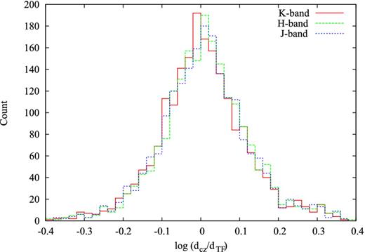
The histogram of logarithmic distance ratios |$\log \frac{d_{cz}}{d_{\mathrm{TF}}}$|. The K-band data is shown by the red solid line, H-band data by the green dashed line, and the J-band data by the blue dotted line.
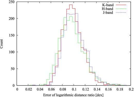
The histogram of the error of the logarithmic distance ratios, using the same colour scheme as in Fig. 5.
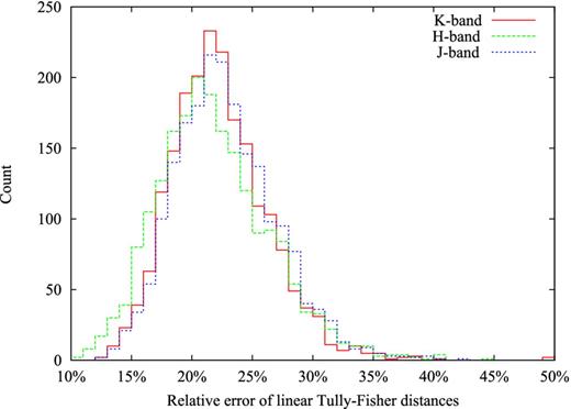
The histogram of the relative errors of linear TF distances, using the same colour scheme as in Fig. 5.
BULK FLOW FITTING AND THE RESULTS
χ2 minimization method
Since the 2MTF sample has a denser galaxy distribution in the sky north of δ = −40°, we introduced the weight |$w^d_i$| to correct the uneven number density in these two sky areas. The regions of the sky north and south of this line contain 1827 and 191 2MTF galaxies and subtend 33 885 and 7368 deg2, respectively. This yields a ratio of galaxy number density between the southern and northern regions of roughly 1:2.08. We therefore set |$w_i^d=2.08$| for the southern objects and |$w_i^d=1$| for the northern ones.
To reduce the effect of outliers, we applied two cuts during the fitting process. With each successive cut, we did the χ2 minimization first, and compared the difference between the bulk flow-corrected logarithmic distance ratio and the predicted Hubble flow logarithmic distance ratio: Δi = log (dz, i/dmodel, i) − log (dz, i/dTF, i). The outliers with Δi > 3σi were then removed. We did the clipping twice, then applied the third χ2 minimization, and report the result as the final bulk flow velocity. The total number of galaxies removed from the sample is around 60.
where N = 50 is the number of jackknife subsamples, |$V_{i}^{J}$| is the bulk flow for the ith jackknife subsample, and |$\overline{V}^J = \frac{1}{N} \sum ^{N}_{i=1} V_{i}^{J}$|. The velocity components in three directions (VX, VY, VZ) were estimated using equation (9).
To analyse the performance of the χ2 minimization method, we simulated 1000 mock catalogues and tested the method with these simulated data. We built the mock catalogues based on the real 2MTF data sample, with each catalogue containing 2018 mock galaxies. These galaxies have the same sky position and redshift as the real 2MTF galaxies. In each mock catalogue, we set the input bulk flow velocity equals to the same value as our measurement of the K-band data sample at the depth of RI = 30 h−1 Mpc, i.e. VX = 163.4 km s−1, VY = −308.3 km s−1, and VZ = 107.7 km s−1. We simulated distance errors by using a Gaussian random variable to induce mock scatter in the TF, with a variance equals to the total logarithmic distance error for that galaxy. The average value of this logarithmic distance error is 0.096, as in the real data.
We fit the bulk flow for each of the 1000 mock catalogues using the χ2 minimization method, and plot the histograms of differences between the input and output bulk flow components VX, VY, and VZ in Fig. 8. We then fit the histograms using Gaussian functions, and found the distribution of 1000 ‘observed’ bulk flow components centred around the input values with a scatter of σX ∼ 35 km s−1, σY ∼ 33 km s−1, and σZ ∼ 25 km s−1, respectively. The distributions present very small shifts of ∼ 2 km s−1 in three components. This is smaller than our quoted bulk flow error by roughly an order of magnitude, and shows that the χ2 minimization method provides an unbiased fit of the bulk flow motion.
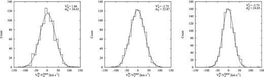
Histograms of the differences between the input and output bulk flow components VX, VY, and VZ for our 1000 mock samples. The solid lines show the best-fitting Gaussians to the distributions. The Gaussian centres are located at |$V_X^c = 1.86$|, |$V_Y^c=-1.75$|, and |$V_Z^c = -1.73$| km s−1 with standard deviations of σX = 34.63, σY = 32.87, and σZ = 24.65 km s−1, respectively.
The best-fitting χ2 bulk flow results are presented in Table 1, subdivided by wavelength and measuring depth RI. In all three bands with three different depths, we detected a non-zero bulk flow with a confidence level of at least 3σ.
Best-fitting χ2 measured bulk flow of the 2MTF sample in J, H, and K bands. The velocity components (VX, VY, VZ) are calculated in Galactic Cartesian coordinates.
| Amplitude | l | b | VX | VY | VZ | χ2/d.o.f. | |
|---|---|---|---|---|---|---|---|
| (km s−1) | (deg) | (deg) | (km s−1) | (km s−1) | (km s−1) | ||
| J band | |||||||
| RI = 20 h−1 Mpc | 303.5 ± 22.2 | 306.7 ± 7.3 | 11.9 ± 4.9 | 177.4 ± 29.2 | −238.2 ± 17.0 | 62.5 ± 22.2 | 0.98 |
| RI = 30 h−1 Mpc | 319.0 ± 28.0 | 297.5 ± 4.1 | 18.5 ± 4.6 | 139.6 ± 17.5 | −268.4 ± 27.9 | 101.1 ± 26.9 | 0.95 |
| RI = 40 h−1 Mpc | 319.4 ± 21.3 | 290.8 ± 4.2 | 11.4 ± 4.7 | 111.3 ± 20.9 | −292.7 ± 19.8 | 63.0 ± 25.6 | 0.95 |
| H band | |||||||
| RI = 20 h−1 Mpc | 345.7 ± 53.6 | 308.7 ± 7.8 | 18.1 ± 13.9 | 205.7 ± 54.4 | −256.3 ± 43.5 | 107.1 ± 82.2 | 1.07 |
| RI = 30 h−1 Mpc | 352.4 ± 34.4 | 296.9 ± 5.6 | 26.8 ± 11.6 | 142.4 ± 29.6 | −280.6 ± 31.7 | 158.7 ± 65.2 | 1.04 |
| RI = 40 h−1 Mpc | 319.1 ± 37.4 | 296.2 ± 8.3 | 5.1 ± 6.1 | 140.5 ± 51.1 | −285.0 ± 28.2 | 28.4 ± 33.6 | 1.00 |
| K band | |||||||
| RI = 20 h−1 Mpc | 301.3 ± 27.3 | 305.4 ± 8.2 | 8.5 ± 6.4 | 172.6 ± 42.1 | −243.0 ± 30.5 | 44.4 ± 39.6 | 1.00 |
| RI = 30 h−1 Mpc | 365.1 ± 36.2 | 297.9 ± 6.1 | 17.2 ± 5.5 | 163.4 ± 36.8 | −308.3 ± 44.5 | 107.7 ± 33.8 | 0.98 |
| RI = 40 h−1 Mpc | 331.1 ± 22.5 | 292.0 ± 3.4 | 11.8 ± 4.2 | 121.4 ± 25.0 | −300.5 ± 19.6 | 67.9 ± 20.8 | 0.96 |
| 3 bands combined | |||||||
| RI = 20 h−1 Mpc | 310.9 ± 33.9 | 287.9 ± 5.9 | 11.1 ± 3.4 | 93.7 ± 34.4 | −290.4 ± 28.9 | 59.8 ± 18.4 | 0.90 |
| RI = 30 h−1 Mpc | 280.8 ± 25.0 | 296.4 ± 16.1 | 19.3 ± 6.3 | 117.8 ± 68.3 | −237.4 ± 30.6 | 92.9 ± 29.4 | 0.93 |
| RI = 40 h−1 Mpc | 292.3 ± 27.8 | 296.5 ± 9.8 | 6.5 ± 9.2 | 129.6 ± 47.6 | −259.9 ± 37.6 | 33.0 ± 46.6 | 0.95 |
In addition to the bulk flow measurements for individual wavebands, we have also combined the data from all three wavebands into a composite measurement of the bulk flow. That is, each galaxy appears in this sample three times, but with different peculiar velocities as measured in each of the wavebands. But we have applied the χ2 minimization method so that each of the three peculiar velocity measurements for a given galaxy is counted separately in equation (6). We then compute the error using the same jackknife method. Though once a galaxy was removed from a subsample, all three peculiar velocities belonging to this galaxy were removed together. We report these composite measurements of the bulk flow as ‘3 bands combined’ in Table 1.
Additional bulk flow fitting methods
Maximum likelihood method
Minimum variance method
The resulting MLE and MV measurements of the bulk flow are presented in Table 2, and they largely agree with the χ2 minimization method. We discuss these results further in the following section.
MV and MLE bulk flow of the 2MTF sample in J, H, and K bands. The errors quoted are noise-only, with noise+cosmic variance in parentheses.
| Amplitude | l | b | VX | VY | VZ | |
|---|---|---|---|---|---|---|
| (km s−1) | (deg) | (deg) | (km s−1) | (km s−1) | (km s−1) | |
| J band | ||||||
| MV (RI = 20 h−1 Mpc) | 313 ± 33(150) | 295 ± 7 | 13 ± 6 | 129 ± 35(174) | −276 ± 33(173) | 71 ± 30(172) |
| MV (RI = 30 h−1 Mpc) | 328 ± 39(137) | 283 ± 7 | 12 ± 6 | 72 ± 39(151) | −313 ± 39(153) | 68 ± 36(150) |
| MV (RI = 40 h−1 Mpc) | 325 ± 49(132) | 275 ± 9 | 7 ± 8 | 27 ± 48(144) | −321 ± 50(147) | 41 ± 45(142) |
| MLE | 351 ± 28 | 295 ± 5 | 17 ± 4 | 143 ± 30 | −304 ± 28 | 100 ± 21 |
| H band | ||||||
| MV (RI = 20 h−1 Mpc) | 294 ± 33(149) | 294 ± 7 | 13 ± 6 | 177 ± 35(173) | −261 ± 33(172) | 67 ± 30(173) |
| MV (RI = 30 h−1 Mpc) | 317 ± 39(135) | 283 ± 7 | 14 ± 7 | 70 ± 39(151) | −300 ± 39(153) | 75 ± 36(150) |
| MV (RI = 40 h−1 Mpc) | 308 ± 48(132) | 275 ± 9 | 10 ± 8 | 29 ± 48(144) | −302 ± 49(147) | 55 ± 45(142) |
| MLE | 338 ± 28 | 294 ± 5 | 18 ± 4 | 133 ± 30 | −292 ± 28 | 104 ± 21 |
| K band | ||||||
| MV (RI = 20 h−1 Mpc) | 305 ± 33(149) | 292 ± 7 | 13 ± 6 | 109 ± 34(172) | −276 ± 33(174) | 71 ± 29(173) |
| MV (RI = 30 h−1 Mpc) | 313 ± 39(134) | 276 ± 7 | 13 ± 7 | 33 ± 39(151) | −303 ± 40(153) | 70 ± 36(149) |
| MV (RI = 40 h−1 Mpc) | 312 ± 49(132) | 270 ± 9 | 11 ± 8 | 1 ± 48(145) | −306 ± 50(147) | 59 ± 45(142) |
| MLE | 345 ± 27 | 295 ± 5 | 16 ± 4 | 141 ± 30 | −300 ± 28 | 95 ± 21 |
DISCUSSION
In Table 1, we list 12 χ2 minimization measured bulk flow velocities from the three 2MASS NIR wavebands and the ‘3 bands combined’ sample, each using three sample depths. To simplify the discussion here, we focus on our best measurements of the bulk flow at the three depths, which are the measurements taken from the combined sample.
Using the combined data with a depth R = 30 h−1 Mpc, we detected a bulk flow velocity in the direction of l = 296| $_{.}^{\circ}$|4 ± 16| $_{.}^{\circ}$|1, b = 19| $_{.}^{\circ}$|3 ± 6| $_{.}^{\circ}$|3. Our direction is consistent with that of most previous studies, but our result tends to have a higher galactic latitude.
We list our χ2 minimization measured bulk flow directions, along with the results from previous studies in Table 3. An Aitoff projection of bulk flow directions is also presented in Fig. 9.
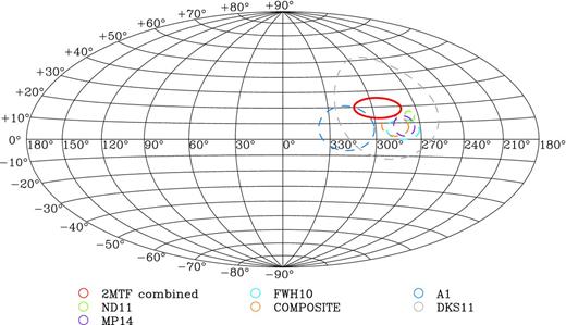
The direction of the measured bulk flow velocities, using an Aitoff projection and Galactic coordinates. The red circle shows the bulk flow direction estimated from ‘3 bands combined’ sample with depth RI = 30 h−1 Mpc. The size of the circles indicates the 1σ error of the direction. The bulk flow directions from several previous studies are also plotted for comparison. The references for these literature results are listed in Table 3.
Bulk flow directions from previous studies.
| l | b | Reference | |
|---|---|---|---|
| (deg) | (deg) | ||
| 2MTF | 296.4 ± 16.1 | 19.3 ± 6.3 | This work |
| COMPOSITE | 287 ± 9 | 8 ± 6 | Watkins et al. (2009) |
| FWH10 | 282 ± 11 | 6 ± 6 | Feldman et al. (2010) |
| ND11 | 276 ± 3 | 14 ± 3 | Nusser & Davis (2011) |
| DKS11 | |$290 ^{+39}_{-31}$| | |$20 ^{+32}_{-32}$| | Dai et al. (2011) |
| A1 | 319 ± 25 | 7 ± 13 | Turnbull et al. (2012) |
| MP14 | 281 ± 7 | |$8 ^{+6}_{-5}$| | Ma & Pan (2014) |
The expected amplitude of the bulk flow is strongly dependent on the characteristic depth of the galaxies being sampled (Li et al. 2012; Ma & Pan 2014). As survey geometry and source selection criteria vary greatly between surveys, one must account for this in comparing the bulk flow amplitude to cosmological expectations.
We show the 3 bands combined measurement of χ2 minimization method in Fig. 10 together with the model predicted curve. The 1σ variance of the bulk flow velocity is also plotted as a dashed line. Our results agree with the model predicted bulk flow amplitude at the 1σ level. Thus, our results support the conclusions reported by some previous studies (e.g. Dai et al. 2011; Nusser & Davis 2011; Turnbull et al. 2012; Kitaura et al. 2012; Rathaus et al. 2013; Ma & Pan 2014) that the bulk flow detected in the local Universe is consistent with the ΛCDM model.
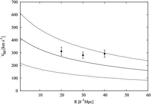
The comparison between the bulk flow velocity amplitude from the 2MTF sample and the ΛCDM prediction using the WMAP-7 yr parameters (Larson et al. 2011). The diamonds with error bars indicate the bulk flow velocity amplitude measured from the 2MTF ‘3 bands combined’ sample using the χ2 minimization method, with the depth RI = 20, 30, and 40 h−1 Mpc, respectively. The solid line shows the theoretical curve and the dashed lines indicate the sample variance at the 1σ level.
As a point of comparison, both the MV and MLE results are shown in Table 2. The MV calculation is performed for the same 20, 30, and 40 h−1 Mpc depths used for the χ2 minimization method, while the MLE method only samples one depth. The measurements largely agree with the χ2 minimization results in both amplitude and direction. A comparison of bulk flow measurements on 2MTF K-band sample is shown in Figs 11 and 12.
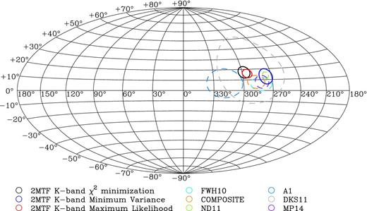
The direction of the measured bulk flow velocities, using an Aitoff projection and Galactic coordinates. The black, blue, and red circles show the bulk flow direction determined from the K-band sample by the χ2 minimization (RI = 30 h−1 Mpc), MV (RI = 30 h−1 Mpc), and maximum likelihood methods, respectively. The size of the circles indicates the 1σ error. The literature bulk flow directions are plotted by dashed circles.
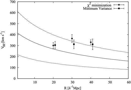
The comparison between the bulk flow amplitudes measured by χ2 minimization method (diamonds) and MV method (squares) on 2MTF K-band sample. The MV method results are shifted 1 h−1 Mpc right to make the comparison clear. The solid line shows the theoretical curve and the dashed lines indicate the variance at the 1σ level.
CONCLUSIONS
The bulk flow motion is the dipole component of the peculiar velocity field, thought to be induced by the gravitational attraction of large-scale structures. Therefore, its measurement can help to constrain cosmological models.
The 2MTF survey is an all-sky TF survey, using photometric data from the 2MASS catalogue and H i data from existing published works and new observations. Using this data set, we have derived peculiar velocities for 2018 galaxies in the local Universe (cz ≤ 10 000 km s−1). This sample covers all of the sky down to a Galactic latitude |b| = 5°, providing better sky-coverage than previous surveys.
We applied a χ2 minimization method to the peculiar velocity catalogue to estimate the bulk flow motion. We applied three Gaussian window functions located at three different depths (RI = 20, 30, and 40 h−1 Mpc) to the catalogues generated by three NIR bands (J, H, and K). Our tightest constraints came from combining the data in all three bands, which gave us bulk flow amplitudes of V = 310.9 ± 33.9, 280.8 ± 25.0, and 292.3 ± 27.8 km s−1 for RI = 20, 30 and 40 h−1 Mpc, respectively. Similar results are found when we apply the maximum likelihood and MV methods of Kaiser (1988) and Watkins et al. (2009), respectively. We find that these amplitudes all agree with the ΛCDM model prediction at the 1σ level. The directions of our estimated bulk flow are also consistent with previous probes.
We gratefully acknowledge Martha Haynes, Riccardo Giovanelli, and the ALFALFA team for supplying the latest ALFALFA survey data. We thank Yin-zhe Ma for useful comments and discussions.
We wish to acknowledge the contributions of John Huchra (1948–2010) to this work. The 2MTF survey was initiated while KLM was a post-doc working with John at Harvard, and its design owes much to his advice and insight. This work was partially supported by NSF grant AST- 0406906 to PI John Huchra.
Parts of this research were conducted by the Australian Research Council Centre of Excellence for All-sky Astrophysics (CAASTRO), through project number CE110001020. TH was supported by the National Natural Science Foundation (NNSF) of China (11103032 and 11303035) and the Young Researcher Grant of National Astronomical Observatories, Chinese Academy of Sciences.
REFERENCES
NEW INTRINSIC ERROR ESTIMATION
As described in Section 2.1, Masters et al. (2008) estimated the intrinsic errors of the TF relation using the 888-galaxy template sample with I-band axis ratio. However, we have adopted the 2MASS co-added axis ratio for the 2MTF sample. Thus, we must make a new estimate of the intrinsic scatter in the TF relation, appropriate for the co-added axis ratio. We have calculated the new intrinsic errors by subtracting the observed error components from the total scatter of the distribution.
The final results are the intrinsic error terms reported by equation (3). We show the error components along with the total scatter of the K-band sample in the Fig. A1. Using the new intrinsic error, the total error closely matches the total scatter.
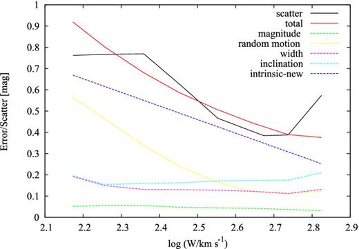
A plot of different error components of the K-band data as a function of the logarithmic H i width. The blue dashed line indicates the new intrinsic error term. The red line shows our estimate of the final total error in the data, which matches the observed scatter of the sample well.
THE RANDOM MOTION OF GALAXIES
Ideally, the intrinsic error of the TF relation would be estimated using a galaxy cluster sample. All of the galaxies in the same cluster are assumed to be at the same distance, thus subtracting out the individual motions of the galaxies themselves. However, when estimating the new intrinsic error term, we used the data of 2018 field galaxies. The uncorrected random motions of these galaxies would introduce a spurious component into the scatter of the TF relation.
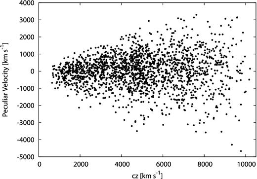
Peculiar velocities versus redshift for the 2018 2MTF field galaxies.
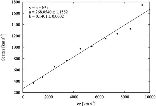
Mean scatter of peculiar velocity as a function of redshift, with the best-fitting linear relation superimposed.
