


Abstract
We carry out high-resolution two-dimensional radiation-hydrodynamic numerical simulations to study the formation and evolution of hot bubbles inside planetary nebulae. We take into account the evolution of the stellar parameters, wind velocity and mass-loss rate from the final thermal pulses during the asymptotic giant branch (AGB) through to the post-AGB stage for a range of initial stellar masses. The instabilities that form at the interface between the hot bubble and the swept-up AGB wind shell lead to hydrodynamical interactions, photoevaporation flows and opacity variations. We explore the effects of hydrodynamical mixing combined with thermal conduction at this interface on the dynamics, photoionization, and emissivity of our models. We find that even models without thermal conduction mix significant amounts of mass into the hot bubble. When thermal conduction is not included, hot gas can leak through the gaps between clumps and filaments in the broken swept-up AGB shell and this depressurises the bubble. The inclusion of thermal conduction evaporates and heats material from the clumpy shell, which expands to seal the gaps, preventing a loss in bubble pressure. The dynamics of bubbles without conduction is dominated by the thermal pressure of the thick photoionized shell, while for bubbles with thermal conduction it is dominated by the hot, shocked wind.
1 INTRODUCTION
Planetary nebulae (PNe) are formed as the result of the evolution of low- and intermediate-mass stars (MZAMS ∼ 1–8 M⊙). In the most simple scenario of the formation of PNe, the star evolves to the asymptotic giant branch (AGB) phase developing a dusty, slow, and dense wind that interacts with the interstellar medium (ISM; e.g. Cox et al. 2012; Mauron, Huggins & Cheung 2013). After the star evolves off the AGB phase towards hotter effective temperatures, the post-AGB star develops a high ultraviolet flux that photoionizes the AGB material. This phase is also characterized by a fast wind that is able to sweep up, shock, and compress the photoionized AGB envelope (Kwok, Purton & Fitzgerald 1978; Balick 1987).
The first report of the detection of X-ray emission associated with a PN was made by de Korte et al. (1985) using observations from the EXOSAT satellite. Since then a great number of PNe have been observed to harbour X-ray emission. A comprehensive review of the PNe reported with the old X-ray facilities (Einstein, EXOSAT, ROSAT, and ASCA) was presented by Chu, Guerrero & Gruendl (2003). Given the capabilities of those satellites, it was not possible to unambiguously disentangle the photospheric emission from the central star (CSPN) from that of the nebular diffuse emission. With the unprecedented sensitivity and angular resolution of the Chandra and XMM–Newton X-ray observatories this problem can finally be resolved. By 2009, diffuse X-ray emission delimited by bright optical bubbles had been reported for 10 PNe (Kastner et al. 2008, and references therein). More recently, Kastner et al. (2012) reported that of the 35 PNe observed to that time with Chandra, ∼30 per cent display diffuse X-ray emission. In all positive detections, the X-ray emission comes from a hot bubble inside an optical shell.
The nature of the diffuse X-ray emission from hot bubbles in PNe is still a matter of discussion. The main problem is that in the wind–wind interaction scenario the shocked plasma would possess temperatures of T ∼ 107–108 K as expected from an adiabatic shocked wind with terminal velocities of v∞ ≳ 103 km s−1 and plasma densities ≲10−2 cm−3. Measured central star wind velocities using P Cygni profiles of UV lines indicate that CSPN wind velocities are generally above 1000 km s−1 and can be as high as 4000 km s−1 (see Guerrero & De Marco 2013). However, the X-ray observations suggest plasma temperatures of TX ∼ 106 K and electron densities of 1–102 cm−3 (Kastner et al. 2012, and references therein).1 It should be noted that the same temperature and density discrepancy is found in hot plasmas detected towards H ii regions and Wolf–Rayet (WR) bubbles (e.g. Güdel et al. 2008; Toalá et al. 2012).
Mellema & Frank (1995) and Mellema (1995) studied the hot bubbles produced in 2D radiation-hydrodynamic simulations of the formation and evolution of aspherical PNe. This pioneering work showed that the interface between the hot bubble and the swept-up shell of AGB material is unstable, but unfortunately the numerical resolution of these simulations was not high enough to fully develop the instabilities. These papers also estimated the soft X-ray emission predicted by the simulations and found that it came from the thin interface between the hot bubble and the surrounding photoionized material where numerical diffusion spreads the temperature and density jumps across four or five computational cells.
More recent numerical models have studied different aspects of the formation of hot bubbles inside PNe and their associated X-ray emission. The influence of the central star stellar wind parameters during the post-AGB phase was studied in purely hydrodynamical, one-dimensional models by Stute & Sahai (2006) and Akashi et al. (2007). They concluded that in this phase the fast wind velocity must be below 103 km s−1 in order to explain such low temperatures in the X-ray-emitting plasma’ however, this is not consistent with the results from the observed P Cygni profiles of UV lines of central star winds. A different explanation for the diffuse emission was put forward in an analytical approach proposed by Lou & Zhai (2010). One difficulty in these works is that they do not take into account the time evolution of the stellar wind properties (velocity and mass-loss rate) and the star's ionizing photon rate.
A more detailed treatment of the evolution of the stellar wind parameters of the central star and the evolution of the X-ray emission from the hot bubble was presented by the Potsdam group in Steffen, Schönberner & Warmuth (2008). They started their 1D study of the evolution of PNe with a parameter study (see Perinotto et al. 1998, 2004) in which they included a large set of initial models from the AGB phase to hot white dwarf (WD) using post-AGB stellar evolution models from Blöcker (1995) and Schönberner (1983). They used three different numerical approaches to the AGB wind evolution: a fixed density profile ρ(r) ∝ r−2, a kinematical approach, and a hydrodynamic calculation. In the two latter cases, the AGB density and velocity profiles depend directly on the evolutionary track used. Specifically, they found that for the hydrodynamical approach, the dependence of the density profile ρ(r) might vary depending on the initial mass from r−1 to r−2.5 with an even steeper gradient (r−3.5) farther from the central star. The transition phase between the AGB and WD phase was developed using the Reimers formulation (Reimers 1975), but they concluded that the dynamical impact of this short-lived phase is rather small. One of their conclusions is that PNe formed from massive central stars will never become optically thin in the high-luminosity phase unless a low-density AGB envelope is developed.
In Steffen et al. (2008), one-dimensional radiation-hydrodynamic models were used to study the effect of classical and saturated thermal conduction on the soft X-ray emission from PNe. The chianti software (Landi et al. 2013) was used to generate synthetic spectra and study the time variation of the luminosities and surface brightness profiles. They concluded that thermal conduction must be taken into account in order to reproduce the observed X-ray luminosities in closed inner cavities in PNe. Since thermal conduction is suppressed perpendicular to the magnetic field direction, this implies that magnetic fields in PNe must be absent or weak (e.g. Soker 1994). These results are consistent both with wind velocities greater than 1000 km s−1 and with the observed soft X-ray emission in PNe having temperatures of a few times T ∼ 106 K. However, the low X-ray temperatures are only obtained if thermal conduction is included – models without conduction fail to reproduce the observations.
An interesting scenario has been presented by Akashi, Meiron & Soker (2008) in which the soft X-ray-emitting gas can be explained as the result of the interaction of a jet with a spherical AGB wind. This model does not take into account the evolution of the central star in any phase nor the ionizing photon flux in the post-AGB phase. The extended soft X-ray emission predicted by this model comes from an expanding bubble of adiabatically cooling shocked jet material, where the jet velocities can lie between ∼500 and 3000 km s−1. The source of the jet is a collimated wind from a binary companion.
This is the first of a series of papers in which we will study the formation, characteristics and evolution of hot bubbles in PNe and their associated soft X-ray emission. Our main goal in this paper is to use 2D axisymmetric numerical simulations to study the formation of the hydrodynamical and ionization instabilities created in the wind–wind interaction between the fast wind and the previously ejected AGB slow wind, and the role played by these instabilities in reducing the temperature at the edge of the diffuse hot bubble. The importance of these instabilities has been downplayed by other authors in earlier one-dimensional numerical treatments of this problem (Villaver, García-Segura & Manchado 2002a; Villaver, Manchado & García-Segura 2002b; Perinotto et al. 2004; Steffen, Schönberner & Warmuth 2008). We find that the instabilities result in density inhomogeneities that become enhanced and can form dense clumps in the region of the contact discontinuity between the shocked fast wind and the swept-up AGB material. Secondary shocks, photoevaporation flows, and photoionization shadows are some of the phenomena associated with the interaction of the fast wind and the ionizing photon flux with these clumps, with consequences both for the hot bubble and for the external photoionized shell. We argue that this highly dynamic mixing region will be an important source of diffuse soft X-ray emission in PNe. We compare the characteristics of models with different initial masses, as more massive stars evolve faster.
The structure of the paper is as follows: in Section 2, we describe the numerical method and the physics included in the simulations, and in Section 3, we present the stellar evolution histories and the stellar wind parameters and ionizing photon rates used as input to the models. Our results are presented in Section 4 and the hot bubble properties and evolution for the cases with and without thermal conduction are discussed in Section 5. In Section 6, we summarize and draw conclusions.
2 NUMERICAL METHOD
The radiation-hydrodynamics numerical scheme used in this work is similar to that used in Toalá & Arthur (2011) and Arthur (2012). The main difference between that scheme and the one used in this paper is the way in which the stellar wind is injected into the computational domain.
2.1 Overview
First, the AGB wind is modelled in 1D spherical symmetry. This is a slow, dense wind expanding at subsonic velocities into the surrounding medium, which results in an r−2 density distribution bounded by a thin, dense shell, located at ≲2 pc as the result of the interaction with the ISM. This shell will not be relevant for the PN formation (see fig. 10 in Villaver et al. 2002b). Variations in the AGB wind parameters during this stage due to thermal pulses can produce internal density structure superimposed on the general r−2 distribution (see Fig. 1). We do not consider the proper motion of the star during this stage, which could lead to anisotropy in the circumstellar medium (see Esquivel et al. 2010; Mohamed, Mackey & Langer 2012; Villaver, Manchado & García-Segura 2012) prior to the onset of the fast wind.
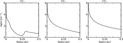
Radial distribution of the number density at the end of the AGB phase for models with initial masses (MZAMS) of 1, 2, and 5 M⊙ zoomed at the inner 0.5 pc as obtained from 1D simulations.
At the end of the AGB stage, the 1D spherically symmetric results are remapped on to a 2D axisymmetric (r, z) grid to continue the evolution through the PN stage, where the effective temperature of the central star increases, resulting in a two-orders of magnitude increase in the stellar wind velocity and the onset of an ionizing photon flux. The combined effects of the fast wind–AGB wind interaction, the density gradient, and the ionizing photon flux lead to the formation of structures at the contact discontinuity due to Rayleigh–Taylor, thin-shell and shadowing instabilities (e.g. García-Segura et al. 1999). These phenomena cannot be modelled in 1D spherical symmetry. The dense clumps formed as a result of these instabilities are ablated and photoevaporated by their interaction with the shocked fast wind and the ionizing photon flux. This leads to a complex scenario in which the densities and temperatures of the material at the edge of the hot, shocked wind bubble do not mark a sharp transition as in the 1D case. In our models, the large surface area presented by these structures formed at the contact discontinuity enhances the evaporation of material from the dense, cold clumps into the hot, tenuous bubble.
2.2 Code description
The hydrodynamic conservation equations are solved using a second-order, finite volume, Godunov-type scheme with outflow-only boundary conditions at the outer boundary. At every time step, the density, momentum and energy in an inner spherical region are reset with a free-flowing stellar wind, whose parameters are interpolated from a table according to the current time values derived from stellar evolution models. The hydrogen ionizing photon rate, S⋆, is also interpolated from these tables and the transfer of ionizing radiation is performed by the method of short characteristics (Raga et al. 1999) in spherical symmetry. This method consists of finding the column density of neutral hydrogen at each point in the grid and thus the optical depth to each point from the ionizing source. A single frequency of ionizing radiation is assumed in these calculations.
The hydrodynamic and ionization equations are coupled through the pressure term in the momentum and energy equations (since the gas pressure depends on the total number of particles, i.e., ions, neutrals, and electrons), and also through the heating and cooling source terms in the energy equation. The hydrogen ionization balance equation (4) is solved and other elements are assumed to be in ionization equilibrium at the temperature and radiation conditions for each computational cell. Although this procedure is not as accurate as taking into account the fully time-dependent ionization of the most important ions (Steffen et al. 2008), it has the benefit of being computationally efficient and is easily extended to two (or more) dimensions.
The radiative cooling term L takes into account abundances appropriate to PNe, via the cloudy PN abundance set (Ferland et al. 2013, see Table 1). These abundances are also used to calculate the appropriate mean nucleon mass. Cooling rates in photoionized gas at temperatures 104–104.5 K are less than in collisionally ionized gas since there will be little Lyα cooling due to the absence of neutral hydrogen. We have generated a table of cooling rates using the cloudy photoionization code for a hot central star with an effective temperature of 100 kK, a mean gas density of 103 cm−3, and an ionizing flux ϕ = S⋆/4πr2 = 1011 cm−2 s−1 (see Fig. 2),2 where r is a representative value of the gas parcel radius inside the nebula. For example, when S⋆ = 1047 s−1, r would be 0.1 pc. In order to avoid spurious cooling due to numerical diffusion at contact discontinuities, we limit cooling in cells whose cooling is more than double that of its neighbours, as described in García-Arredondo, Arthur & Henney (2002). The heating term, G, depends on the local photoionization rate and the current stellar effective temperature.
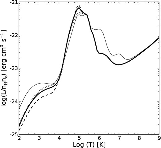
Cooling rate per hydrogen nucleon for gas in a photoionizing radiation field obtained from cloudy (see the text for details). Dotted, solid, and dashed lines correspond to stars with effective temperatures of 50, 100, and 150 kK, respectively, computed with typical PNe abundances (see Table 1). The thin line corresponds to a stellar effective temperature of 40 kK and ISM abundances.
Abundance set for a PN and the interstellar medium (ISM) in cloudy.a
| Atom | PN | ISM |
|---|---|---|
| (logX+12) | (logX+12) | |
| He | 11.0 | 10.991 |
| C | 8.892 | 8.399 |
| N | 8.255 | 7.899 |
| O | 8.643 | 8.504 |
| F | 5.477 | 4.301 |
| Ne | 8.041 | 8.090 |
| Na | 6.279 | 5.500 |
| Mg | 6.204 | 7.100 |
| Al | 5.431 | 4.900 |
| Si | 7.00 | 6.500 |
| P | 5.301 | 5.204 |
| S | 7.00 | 7.511 |
| Cl | 5.230 | 5.000 |
| Ar | 6.431 | 6.450 |
| K | 5.079 | 4.041 |
| Ca | 4.079 | 2.612 |
| Fe | 5.699 | 5.800 |
| Ni | 4.255 | 4.266 |
aFrom Ferland et al. (2013).
The 1D numerical scheme is used to simulate the evolution through to the end of the AGB stage. The AGB stage is deemed to end once the stellar effective temperature is more than 104 K and the ionizing photon rate rises steeply. At this point, the 1D distributions of density, momentum and total energy are remapped to a 2D cylindrically symmetric grid using a volume-weighted averaging procedure to ensure conservation of these quantities. The calculation then proceeds in 2D but we also continue the 1D calculation for comparison.
The 2D cylindrically symmetric hydrodynamic conservation equations are solved using a hybrid scheme, in which alternate time steps are calculated by a second-order Godunov-type method and the van Leer flux-vector splitting method (van Leer 1982). The outer r and z boundaries are outflow only, while the radial fluxes are zero at the symmetry axis.
In an analogous fashion to the 1D case, the stellar wind is input into the computational domain as a free-flowing wind in an inner spherical region, which is reset at every time step with the appropriate values interpolated from the stellar evolution table. The radiation transport is performed by the 2D axisymmetric version of the same short characteristics method and the source of ionization (the star) is taken to be positioned on the symmetry axis. In the same way, the hydrodynamic and ionization equations are coupled through the pressure term in the momenta and energy equations and through the source term in the energy equation. We again solve the time-dependent hydrogen ionization equation (4) and employ the 2D advection equation to describe the transport of the neutral hydrogen fraction through the computational domain. We use the same radiative cooling source term and again limit the cooling in a cell whose cooling is more than double that of its neighbours in an effort to avoid spurious cooling due to numerical diffusion in the vicinity of contact discontinuities. We optionally include thermal conduction through the axisymmetric diffusion equation (5), which is again solved by appropriate numerical techniques through operator splitting after the main hydrodynamic and radiation transport steps.
2.3 Computational grid and initial conditions
For the 1D spherically symmetric calculations, the initial conditions for the ISM are a density of n0 = 1 cm−3 and a temperature of T0 = 100 K. The initial grid has 2000 uniformly spaced radial cells and the initial spatial size is 0.5 pc. The wind injection zone comprises the innermost 10 cells. The computer code automatically detects when the outer edge of the expanding AGB wind has become close to the outer boundary and incrementally extends the computational grid with more cells at the original initial conditions of density and temperature whenever necessary. This procedure avoids large computational domains at the beginning of the simulation and also means that the final size depends on the particular stellar evolution model being calculated without needing to compromise the initial resolution.
The 2D axisymmetric calculations are performed on a fixed grid of 1000 radial by 2000 z-direction cells of uniform cell size and total grid spatial extent 0.5 × 1 pc2. The initial conditions for these calculations are the remapped results of the innermost 0.5 pc of the 1D calculations, which entirely fill the 2D computational domain. The free-wind injection region has a radius of 40 cells, corresponding to 0.02 pc. With this number of cells, the spherical free-wind injection region can be adequately represented on the axisymmetric grid. The use of a fixed-size grid has the disadvantage that, for the lowest initial stellar mass models, the outer photoionized shell leaves the computational domain at late times. However, since we are primarily interested in the formation of hot bubbles and their potential for emitting soft X-rays, we have decided to focus on the region (r2 + z2)0.5 < 0.5 pc.
The remap to the 2D grid also downgrades the numerical resolution since the 2D calculations are computationally far more expensive than the 1D calculations. In order to provide a meaningful comparison with 1D results, we also downgrade the resolution of the continuing 1D simulations and fix the total number of radial cells to 1000.
3 STELLAR EVOLUTION MODELS
In this paper, we use publicly available stellar evolution models with initial masses of 1, 1.5, 2, 2.5, 3.5, and 5 M⊙ at solar metallicity (Z = 0.016) from Vassiliadis & Wood (1993) for the AGB phase and from Vassiliadis & Wood (1994) for the post-AGB phase (see Fig. 3). These models correspond to final WD masses of 0.569, 0.597, 0.633, 0.677, 0.754, and 0.90 M⊙. We will label each set of simulation as a combination of their initial masses and the final WD mass, for example, the model with initial mass of 1 M⊙ and final WD mass of 0.569 M⊙ will be called 1.0–0.569. Thus, the full set of models will be referred as 1.0–0.569, 1.5–0.597, 2.0–0.633, 2.5–0.677, 3.5–0.754, and 5.0–0.90.
![Evolutionary tracks for the WD models from Vassiliadis & Wood (1994) used in this paper. The positions of the (black) circles mark times at [1, 5, 10, and 20] × 103 yr on the tracks. Stars (red) and diamonds (blue) indicate the positions on the tracks when the 2D hot bubble has a mean radius of ∼0.2 pc (or the maximum extension in the case of the most massive models), for cases without and with thermal conduction, respectively.](https://oup.silverchair-cdn.com/oup/backfile/Content_public/Journal/mnras/443/4/10.1093/mnras/stu1360/3/m_stu1360fig3.jpeg?Expires=1716438710&Signature=kWM~v7BrI5ibpjvUdMRPLvz~kVHES3s9t6QYwMnmAOYRg4NNcB4qc7whKd1qVahBN7zcogH9HtrJTNwt7lMiT5f90ZHz6ROpFys-3hVGjwQIN52cpd88nczIwr2zMK5khxG7Ym~1zokwKx3VC1RcucJsi0yHZl9h7NWbHlwyx1upPs5lUzkTFpbkLGHfCS9cH7NvbHfrleRHHQN8f19~71oAkGWz-9jZJQRWxdVGfYVMkLCyZwkzgOix0-kHScjZrW1SdUHof-1tVl2yPKfdCohl4w2bTTYzuWrDQBjSVYbzg30e1v00Z7ui5WnNwbEQIM9BCjbJPw1Qxn0Va3xxug__&Key-Pair-Id=APKAIE5G5CRDK6RD3PGA)
Evolutionary tracks for the WD models from Vassiliadis & Wood (1994) used in this paper. The positions of the (black) circles mark times at [1, 5, 10, and 20] × 103 yr on the tracks. Stars (red) and diamonds (blue) indicate the positions on the tracks when the 2D hot bubble has a mean radius of ∼0.2 pc (or the maximum extension in the case of the most massive models), for cases without and with thermal conduction, respectively.
The AGB wind parameters (velocity and mass-loss rate) are empirical relations derived by Vassiliadis & Wood (1993) from observations of Galactic and Large Magellanic Cloud Mira variables and dust-enshrouded AGB stars and are the same as those used by Villaver et al. (2002a). The stellar wind parameters and ionizing photon flux during the hot CSPN stage were computed using the wm-basic hot star stellar atmosphere code (Pauldrach, Puls & Kudritzki 1986; Pauldrach 1987; Pauldrach et al. 1994; Pauldrach, Hoffmann & Lennon 2001; Pauldrach, Vanbeveren & Hoffmann 2012) using the stellar effective temperature, radius, and surface gravity taken at discrete times from the stellar evolution models from Vassiliadis & Wood (1994). Fig. 4 (top panels) shows the mass-loss rates and velocity profiles corresponding to the CSPN stage for the six evolution models. An improvement between our stellar parameters and those from previous numerical studies is that we do not model the ionizing photon flux as blackbody radiation. With the use of wm-basic, we obtained realistic spectra at different evolution times of the star and we integrated them to compute the ionizing photon rate. Fig. 4 (bottom-left panel) shows the resultant integrated ionizing photon flux for the six models studied here. As the star becomes hotter and more compact, the opacity increases and the ionizing photon flux diminishes considerably compared to a blackbody (see Fig. 4, bottom-right panel).
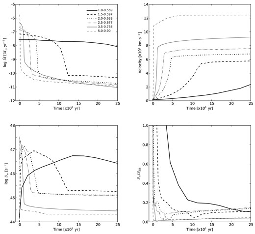
Top left: mass-loss rate; top right: stellar wind velocity; and bottom left: ionizing photon flux for the different stellar models. Bottom right: ratio of the ionizing photon flux over that expected from a blackbody model. The initial–final mass of each model is marked on top-left panel.
As can be seen from Fig. 4, the potential lifetime of a PN produced by a star of initial mass 5.0–0.90 M⊙ is considerably shorter than that of a 1.0–0.569 M⊙ star.
In common with Villaver et al. (2002b), we assume that the post-AGB stage starts when the star's effective temperature has reached 104 K and we do not model the short transition phase between the superwind and the post-AGB phase. We are aware that the inclusion of this transition may affect the hydrodynamics at the edge of the hot bubble (Perinotto et al. 2004).
4 RESULTS
We will separate the presentation of the results into two groups according to similarities in the morphological evolution. This is mainly a consequence of the density structure at the end of the AGB stage (see Fig. 1) and the duration of the CSPN stage. Group A comprises the results from 1.0–0.569M⊙, 1.5–0.597 M⊙, 2.0–0.633 M⊙, and 2.5–0.677 M⊙ stars, while Group B consists of the 3.5–0.754 M⊙ and 5.0–0.90 M⊙ stars. The Group A models start with a circumstellar medium whose density falls off quite steeply with distance from the star. Group B models have a less steep fall off in the initial density distribution and are therefore denser at a given radius. At early times, all the models create well-defined hot bubbles with sharp shells but soon differences in the stellar wind parameters, the circumstellar medium left by the AGB stage, the ionizing photon rate variation, and the different evolution time-scales lead to significant morphological differences. We first describe the results without thermal conduction, and then discuss the main features of the inclusion of this physical effect.
All our models focus on the innermost 0.5 pc of the PN, since this is the region that hosts the hot bubble. As a result, we do not follow the complete evolution of the PN, since at late times the photoionized outer shell leaves the computational domain. We present a series of images for each model, corresponding to the inner hot shocked wind bubble having mean radius 0.05, 0.1, and 0.2 pc for Group A models, and for the Group B models we show results corresponding to the maximum radius of the hot, shocked bubble, since in these cases the hot bubble stalls before it reaches 0.2 pc and then begins to collapse. In order to highlight the main features of each group, we show figures for representative models in the main text, and figures for the other models are collected in Appendix A. For Group A, the representatives are 1.5–0.597 M⊙ and 2.5–0.677 M⊙ (see Figs 5 and 6), while for Group B the representative is 3.5–0.754 M⊙ (see Fig. 7).
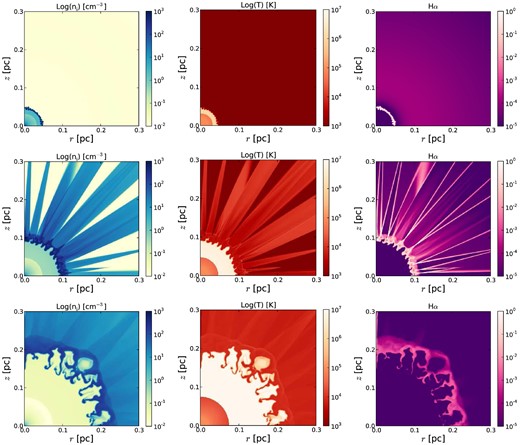
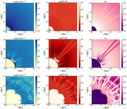
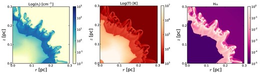
Total ionized number density (left-hand panels), temperature (middle panels) and normalized Hα volume emissivity (right-hand panels) for the PN formation for the 1.5–0.597 model 2D simulations without thermal conduction. The rows correspond to the hot bubble having a mean radius of, from top to bottom, 0.05, 0.1 and 0.2 pc. These are equivalent to 1000, 3500, and 7400 yr of post-AGB evolution for this CSPN. The bottom row corresponds to the time when the central star has an effective temperature and luminosity of Teff = 97 720 K and L = 4310 L⊙.
Same as Fig. 5 but for the case of 2.5–0.677 model without thermal conduction. The rows correspond to the hot bubble having a mean radius of, from top to bottom, 0.05, 0.1, and 0.2 pc. These are equivalent to 1800, 2930, and 7300 yr of post-AGB evolution for this CSPN. The bottom row corresponds to the time when the central star has an effective temperature and luminosity of Teff = 127 640 K and L = 165 L⊙.
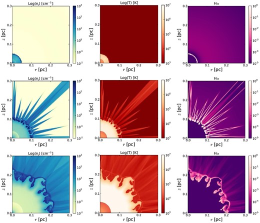
Same as Fig. 5 but for the case of 3.5–0.754 model without thermal conduction. This set of panels corresponds to the maximum radius of the hot bubble, which occurs after 4900 yr of post-AGB evolution for this CSPN. The panels corresponds to the time when the central star has an effective temperature and luminosity of Teff = 162 180 K and L = 250 L⊙.
In each set of images, the total ionized number density (ni = ρyi/μmH, where μ mean particle mass), temperature, and Hα emitting region are shown.3 Although the calculations are performed on the full r-z plane, the results are symmetric about the mid-plane and for reasons of space, we show only half of the computational domain.
4.1 Group A
Models 1.0–0.569, 1.5–0.597, 2.0–0.633, and 2.5–0.677 evolve in very similar ways due to the similarity of the initial circumstellar medium density distribution and velocity at the start of the post-AGB phase (see Fig. 1). These models follow the classic PNe formation scheme: the fast CSPN wind expands into the slowly expanding vexp ≲ 15 km s−1, smooth ρ ∝ r−2 (or steeper) density profile left after the AGB stage. The interaction between the fast wind and the slow wind forms a two-shock pattern: the outer shock sweeps up and compresses the AGB material, while the inner shock brakes and heats the fast wind. The two shocks are separated by a contact discontinuity. Behind the outer shock, the density is very high and cooling is efficient. The thin-shell instability (Vishniac 1983; Vishniac & Ryu 1989) acts at early times to corrugate the contact discontinuity separating the cold, dense material from the hot bubble and clumps begin to form (see the upper panels in Figs 5 and 6).
The ionization front is initially trapped close to the thin shell, but as the shell moves outwards the opacity falls and the ionization front progresses outwards. The clumps formed by the instability lead to variations in the opacity and as a consequence the shadowing instability becomes important at later times (Williams 1999). Characteristic rays of alternating ionized and neutral material form at intermediate times. These can be visualized as bright streaks in the Hα volume emissivity trailing from bright Hα clumps, as can be seen in the central panels of Figs 5, 6, and the Group A models in Appendix A. At later times, the opacity in the ring of clumps drops as they expand outwards, and the whole outer region becomes photoionized and more homogeneous.
The continued acceleration of the fast stellar wind means that the swept-up shell is accelerated down the density gradient and Rayleigh–Taylor instabilities become important at the contact discontinuity between the low density, shocked fast wind material and the dense, swept-up shell. This leads to the formation of elongated, dense, partially ionized structures pointing inwards into the hot bubble. Neutral, dense material inside these filaments can be photoevaporated by the ionizing flux. The expanding, photoevaporated gas flows away from the head of the neutral filament, towards the central star. It then interacts dynamically with the radially outflowing, shocked fast wind, giving rise to pockets of ∼106 K gas with densities in the range 0.1 < ni < 1.0 cm−3. The hot bubble, on the other hand, has temperature >107 K and density ni < 0.01 cm−3. Even when there is no neutral material inside the dense filaments to generate photoevaporated flows, the diversion of the shocked fast wind material around the dense obstacles leads to hydrodynamic ablation and the mixing of cooler, dense material into the faster, hot flow (see e.g. Hartquist et al. 1986). In general, the models that evolve more slowly generate longer filamentary structures, simply because they have had a much longer time to grow by the time the hot bubble has expanded to 0.2 pc radius.
The 2.5–0.677 case is particularly interesting. The ring of clumps forms due to the thin-shell instability as for the other cases in this group. However, the faster acceleration of the stellar wind and the resulting higher pressure in the hot bubble mean that the clumps are pushed out to about 0.1 pc before the photoionization has the opportunity to cause this shell of swept-up material to expand. The clumps are therefore denser in this model at this radius than for other models. The ionizing photon rate of the central star now drops sharply and so the dense clump material recombines. This leads to the situation where the heads of the now neutral clumps develop ionization fronts and photoevaporation flows pointing towards the central star. Initially, the pressure of the hot bubble is higher than the pressure in the photoionized material, and the photoevaporated material is pushed back into the shell. As the whole structure expands slowly outwards, however, and the mass-loss rate of the central star drops sharply, the pressure in the photoevaporated flows becomes greater than that in the hot bubble and starts to expand away from the neutral clumps, back towards the central star after passing through a termination shock. This leads to the situation in the final row of Fig. 6, where the hot bubble is surrounded by a thick shell of photoionized material, within which are embedded neutral clumps. The thick shell is slowly moving outwards, broadening as it goes, and the hot bubble is confined by the slowly decreasing pressure of the photoionized gas.
Structures similar to those shown in Figs 5, 6, and A1, i.e. a hot inner cavity surrounded by lacy structures in turn surrounded by a smooth photoionized shell, are observed in Hubble Space Telescope (HST) images of, e.g. IC 418, NGC 2392, NGC 6826, and NGC 7662, which also display inner diffuse X-ray emission surrounded by a photoionized shell detected with Chandra (Kastner et al. 2012; Ruiz et al. 2013).
4.2 Group B (3.5–0.754 and 5.0–0.90)
Models from Group B are the result of the evolution of the most massive stars of our sample. The density distribution around these stars at the end of the AGB stage does not have such a steep radial dependence. This means that the fast wind expands into a denser medium and the swept-up shell of AGB material is correspondingly denser. In fact, the ionization front becomes trapped in the shell and does not manage to break out and hence the surrounding medium remains neutral throughout the evolution. The photoionized shell has a high thermal pressure and effectively confines the hot bubble to small radii. This effect is enhanced by the sharp CSPN mass-loss rate fall off (see Fig. 4, top-left panel) and as a consequence, the thermal pressure of the hot bubble decreases with time. There comes a point when the pressure inside the hot bubble becomes lower than that in the surrounding photoionized shell. This marks the point at which the hot bubble ceases to expand and starts to collapse. In Figs 7 and A1, we show the maximum extent of the hot bubble for these models. As can be seen, the hot bubble is surrounded by a thick photoionized shell and this is embedded within a dense neutral envelope.
4.3 Thermal conduction results
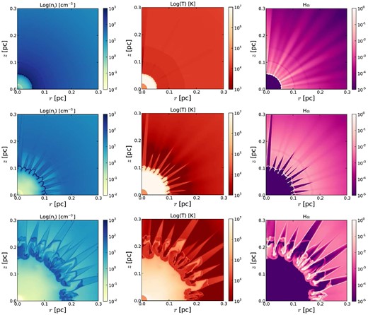
Figs 8 –10 (and see also Fig. A2, Appendix A) show the corresponding results for the cases with thermal conduction. Conduction by thermal electrons heats material from the dense, cool, swept-up AGB shell and it then expands into the hot bubble. The evaporation process results in a sheath of comparatively dense (ni ∼ 1 cm−3), but hot (105 < T < 106 K) material around the fingers and clumps that were formed by the different instabilities at the interface between the hot bubble and dense swept-up shell. The total surface area of the conducting layer is very large because of these instabilities and substantial amounts of AGB shell material are evaporated into the hot bubble.
Same as Fig. 5 but for the 1.5–0.597 model with thermal conduction. The rows correspond to the hot bubble having a mean radius of, from top to bottom, 0.05, 0.1, and 0.2 pc. These are equivalent to 1000, 3200, and 6200 yr of post-AGB evolution for this CSPN. The bottom row corresponds to the time when the central star has an effective temperature and luminosity of Teff = 90 160 K and L = 4610 L⊙.
Same as Fig. 5 but for the case of 2.5–0.677 model with thermal conduction. The rows correspond to the hot bubble having a mean radius of, from top to bottom, 0.05, 0.1, and 0.2 pc. These are equivalent to 1800, 2500, and 4300 yr of post-AGB evolution for this CSPN. The bottom row corresponds to the time when the central star has an effective temperature and luminosity of Teff = 142 900 K and L = 295 L⊙.
Same as Fig. 5 but for the case of 3.5–0.754 model with thermal conduction. This set of panels corresponds to the maximum radius of the hot bubble, which occurs after 5500 yr of post-AGB evolution for this CSPN. The panels corresponds to the time when the central star has an effective temperature and luminosity of Teff = 158 500 K and L = 240 L⊙.
We find that the pressure in the hot bubble is higher in the models with conduction and so the expansion for all models is more rapid than for the models without conduction. This is because the evaporated material expands into the interclump region between the clumps and filaments in the broken shell and the bubble does not depressurize. At a given time, the instabilities are much more developed for the models with conduction than those without. The swept-up photoionized shells in the models with conduction are thinner because the hot bubble dominates the dynamics. The higher pressure means that these PNe are essentially wind-blown bubbles surrounded by thin swept-up shells. The models without conduction, on the other hand, have their dynamics dictated by the pressure in the broad photoionized shell (see e.g. Arthur 2012; Raga, Cantó & Rodríguez 2012).
4.4 Comparison between 2D and 1D results
In Fig. 11, we compare the 2D results shown in the previous sections to the corresponding 1D results calculated at the same numerical resolution and with the same physical processes. In order to make the comparison, we plot the 2D results as a function of radial distance from the star averaged over all angles. The top row of figures shows the averaged 2D results without conduction for the three principal models: 1.5–0.597, 2.5–0.677, and 3.5–0.754 and the bottom row shows the results when thermal conduction is included. Each figure also shows the 1D simulation results both with and without conduction at the same evolution times. The upper panel in each figure is the total number density (n = ρ/μmH), the centre panel is the temperature, and the lower panel shows the value of a passive advected scalar. This scalar is assigned a value of one in the AGB wind material prior to the onset of the fast wind, and is zero in the post-AGB fast-wind material that enters the grid thereafter. Intermediate values indicate mixed regions: for the 1D simulations this is an indication of a cooling region, for the 2D simulations it is a result of the averaging process. The scalar shows how far the evaporated dense shell material has penetrated into the hot bubble.
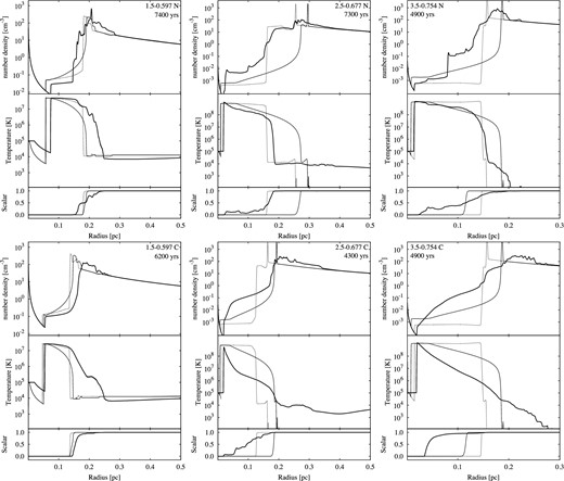
Comparison of 2D results with 1D results. Top row – 2D results without thermal conduction. Bottom row – 2D results with thermal conduction. In each plot, the upper panel shows the total number density (n = ρ/μmH) and the centre panel shows the temperature. The lower panel shows the value of a passive advected scalar. The thick solid line is the 2D simulation as a function of radius averaged over all angles from the stellar position. The thin solid line is the 1D result with thermal conduction and the dotted line is the 1D result without thermal conduction, both at the same evolution time as the corresponding 2D result.
We begin with an explanation of the 1D results. The classical description of a stellar wind bubble divides it into distinct regions (see e.g. Dyson & Williams 1997; Arthur 2012). Closest to the star, there is an inner region of unshocked, free-flowing stellar wind, which is separated from the hot bubble by an inward-facing shock. The hot bubble comprises hot, shocked stellar wind material and is separated by a contact discontinuity from the swept-up shell. This shell is composed of swept-up ambient medium, which for our models is AGB material. There can be a photoionized region inside the swept-up shell, in which case there will be an ionization front preceded by a shock in the neutral medium within the shell. External to the shell is undisturbed ambient medium. For a steady stellar wind, the pressure between the inner stellar wind shock and the outer neutral shock will be uniform. The contact discontinuity between the hot, shocked stellar wind and the swept-up, photoionized shell separates diffuse gas at ∼107 K from dense gas at ∼104 K. If magnetic fields are not important at this interface, conduction due to thermal electrons from the hot gas can lead to diffusion of heat across the contact discontinuity (see equation 5). For the hot, diffuse gas, the heat diffusion leads to a loss of thermal energy and hence a reduction of temperature in this gas together with a corresponding increase in density, since the pressure remains constant. For the cooler, dense gas, there is an increase in temperature. Depending on the details of the radiative cooling, the stellar wind, and the ionizing photon rate, one of the following must occur:
The cooling time-scale for the heated dense material is so short that it cools immediately back to its original state. We remark that this case is also likely to occur if there is over cooling at the contact discontinuity as a result of numerical diffusion.
The heated dense gas expands at constant pressure, where the pressure is dictated by conditions in the hot shocked wind bubble. The increase in volume (and corresponding decrease in density) in this gas pushes the shell outwards.
The heated dense gas cannot expand outwards and instead pushes inwards, increasing the pressure inside the hot, shocked bubble and pushing the inner stellar-wind shock closer to the star. This occurs particularly if the stellar wind mechanical energy is decreasing rapidly with time.
Whichever of these three behaviours prevails initially, radiative cooling will play an important rôle on the time-scale of a cooling time. Cooling times are shortest in the heated dense region. As this gas begins to cool, its volume decreases (since the pressure must remain constant because this gas is located between the hot, shocked bubble and the surrounding photoionized region). Due to the short evolution time-scales of these PN models, cooling is not necessarily complete on the time-scale of the simulations. We see evidence for a cooling region in the 1.5–0.597 1D model results (see Fig. 11). Cooling in the reduced temperature diffuse gas occurs on much longer time-scales (see e.g. Arthur 2012).
Fig. 11 shows examples of the second and third types of situations listed above. For example, the 1.5–0.597 models are examples of the second case, where in the models with conduction, the heated, dense gas expands and pushes the dense shell outwards, in comparison with the models without conduction. In these models, the ambient medium gas is photoionized beyond the swept-up shell. The 3.5–0.754 models, on the other hand, are examples of the third case, where the heated dense gas expands quite a long way back towards the star, pushing the inner stellar wind shock to smaller radii in the models with conduction, in comparison with the models without conduction. In these models, the swept-up shell of ambient medium gas is mainly neutral, since the ionizing photon rate falls off rapidly within the first 1000 yr of the PN evolution. The scalar in these figures indicates the position of the interface between the wind material and the ambient material. The 2.5–0.677 models are more complicated, since the swept-up shell contains the ionization front and preceding neutral shock and is mainly, though not completely, photoionized. The photoionized gas regulates the pressure throughout the PN once the stellar wind mechanical luminosity begins to decline.
We now examine the differences between the 2D and 1D simulations.4 For the 1.5–0.597 case without conduction, we immediately notice that the inner stellar wind shock for the angle-averaged 2D results is at a larger radius than for the equivalent 1D models. This means that the density, and hence, the pressure in the hot, shocked wind bubble is lower in the 2D case, since the post-shock temperature is the same in all cases because it depends only on the stellar wind velocity. The reason for the lower pressure can be appreciated by looking at Fig. 5. The swept-up shell in this figure has broken up due to instabilities and the hot wind can find its way through the gaps, depressurizing the hot bubble. Although the peak density occurs at roughly the same radius as in the 1D models, warm (T > 104 K) gas extends beyond the shell as a result of mass pick-up from the clumps and filaments by the hot wind as it flows through the gaps in the leaky bubble. For the 1.5–0.597 2D model with conduction, the inner stellar wind shock coincides more-or-less with the 1D results. This is because conduction heats the gas at the surface of the cold, dense filaments and the expansion of this gas seals the gaps in the bubble. The result is a broad, roughly uniform density shell with a temperature of a few times 105 K.
The averaged locations of the interface between hot bubble and swept-up shell in 2.5–0.677 2D models with and without conduction correspond roughly to their 1D counterparts. However, the average density as a function of radius within the hot bubble is an order of magnitude higher in both cases. This is a result of hydrodynamical mixing of dense material into the hot diffuse gas at the irregular interface. Non-radial motions thoroughly mix the ablated, cool, dense gas throughout the hot bubble, thereby raising the average density and lowering the average temperature. This is in contrast to the 1D conduction results, where the temperature in the hot bubble is reduced solely as a result of heat loss due to diffusion of heat, with no corresponding diffusion of material. The averaged 2D models have lower density, broader, swept-up shells than the 1D models, and opacity variations in these shells between the clump and interclump gas mean than photons can leak through into the surrounding ambient medium. In the 1D cases, the photoionized region remains trapped in the swept-up shell.
The results for the 3.5–0.754 2D model without conduction are similar to their 1D counterpart. The average density inside the hot bubble is dominated by the long, dense filament that can be seen in Fig. 7 extending inwards from the interface. The swept-up shell is far broader and has a much lower density than in the 1D models and is partially ionized. In the 2D model with conduction, the interface is extremely distorted (see Fig. 10) and this makes it difficult to identify in the averaged density and temperature plots.
4.5 Hot bubble mass
The clumps and filaments formed by the instabilities at the interface between the hot, shocked fast wind and the dense, photoionized shell are sources of mass for the hot bubble. Hydrodynamic ablation and photoevaporation remove material from the dense structures, which then shocks against and mixes into the hot shocked wind (Steffen & López 2004). The mass of hot gas (where we consider T > 8 × 10⁴ K to be ‘hot’) is thus not solely due to the mass lost by the post-AGB star. Thermal conduction can also enhance the mass of gas in the hot bubble by directly evaporating photoionized shell material at the interface. The increased surface area due to the corrugations in the interface facilitates the mixing processes.
To illustrate this, we compute the mass of hot gas in the bubble as a function of time for the 1.5–0.597 and 2.0–0.633 models (the other cases are similar) for the first 8000 yr of the PNe. Fig. 12 shows the total mass injected by the post-AGB wind, obtained by integrating the mass-loss rates shown in Fig. 4 and the actual mass of hot gas in the numerical simulation for both models and for the simulations with and without thermal conduction. It is clear that the hot bubble becomes dominated by mixed-in mass even in the 2D simulations without conduction. For the 1.5–0.597 model, this occurs after 5500 yr when there is no conduction, and almost from the outset in the model with conduction. For the 2.0–0.633 model, the mixed-in mass dominates after 2500 yr in the case without conduction. In contrast, the 1D model for the 1.5–0.597 case without conduction shows that the hot bubble mass is always less massive than the total injected wind mass, which is what one would expect for the case with no mixing. The hot bubble mass for our 1D model for the 1.5–0.597 case with conduction shows similar behaviour to the comparable model of Steffen et al. (2008), although a direct comparison is not possible due to the different stellar wind properties adopted in the two models. Our 2D models show that for the times when the hot bubble has reached a radius of 0.2 pc, even the cases without thermal conduction are dominated by mixed-in mass. When thermal conduction is included, there is an order of magnitude more mixed-in mass in the hot bubble.
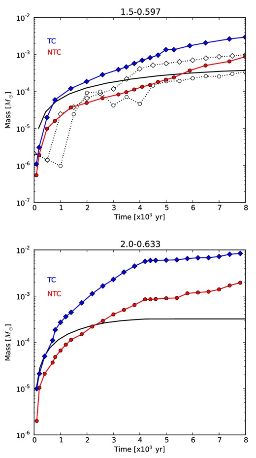
The hot bubble mass as a function of time for the 1.5–0.597 and 2.0–0.633 models. The solid lines without symbols represent the amount of mass injected by the fast wind. The lines with circles (red) represent the total mass of the hot bubble without thermal conduction, while the diamonds (blue) represent the model with thermal conduction. Dotted lines with open symbols represent the corresponding 1D results for the 1.5–0.597 models only.
The increase in the mass of hot gas in the PNe in these 2D simulations as compared to our 1D models (see also the 1D simulations of Steffen et al. 2008) suggests that detection in soft X-rays is likely even when thermal conduction is not present. We address this issue in a forthcoming paper (Paper II, Toalá & Arthur in preparation).
4.6 Photoionized shell expansion velocity
The radial velocity of the photoionized shell is of observational and theoretical interest (Villaver et al. 2002b; Perinotto et al. 2004; Schönberner, Jacob & Steffen 2005; García-Segura et al. 2006; Pereyra, Richer & López 2013) since it provides a link between observable properties of the PN and the evolution of the central star. The photoionized shell kinematics depends on the initial density distribution left by the AGB star, the stellar wind mechanical energy and the stellar ionizing photon luminosity. Our simulations are focused on the formation of the hot bubble (see Section 2.3), and our spatial domain extends only to 0.5 pc radius from the star. As a result, at late times, we lose information about the outer shell that results from the ionization front and its interaction with the outer rim of the AGB material. However, we can study the expansion velocity of the dense shell created in the fast wind–AGB wind interaction. This dense shell, or W-shell (see Mellema 1995), is created by the expansion of the hot shocked wind into the photoionized AGB material.
Fig. 13 shows the W-shell velocity as a function of time for the 1.5–0.597 and 2.0–0.633 models with and without thermal conduction. All models show a steady increase of the W-shell velocity with time, which is consistent with previous numerical results by Schönberner et al. (2005). Observational results (Pereyra et al. 2013) suggest that the nebular shells decelerate as the central star luminosity decreases; however, we do not find this from our 2D models. Our models with thermal conduction have, in general, faster expansion rates, since the pressure in the hot bubble is higher in these models than in those without conduction. We do not calculate the nebular expansion for the 3.5–0.754 and 5.0–0.90 models as these would not be observationally detected since they are ionization bounded and enshrouded by dense neutral material.
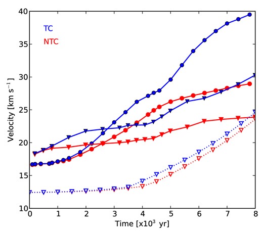
W-shell velocity as a function of time for the 1.5–0.597 (triangles) and 2.0–0.633 (circles) models. Models including thermal conduction are represented with filled (red) markers. The corresponding 1D results for the 1.5–0.597 model are shown with dotted lines and open triangles.
5 DISCUSSION
The results presented in Section 4 illustrate the formation of hot bubbles for different initial-mass stellar-evolution models. Instabilities corrugate the interface between the hot bubble and the surrounding dense shell and lead to the formation of filaments and clumps. The properties of these clumps depend on the interplay between the initial AGB density profile and the time-dependence of the stellar wind and ionizing photon rate in the post-AGB phase. The stellar wind velocity increases steadily with time for CSPN masses <0.754 M⊙), and so the temperature of the hot, shocked stellar wind increases during the PN lifetime. In the case of the 1.0–0.569 M⊙ model, the velocity increases extremely slowly, and the temperature in the hot bubble is only T ∼ 106 K even after 5000 yr of PN evolution. On the other hand, the velocity increase in the 2.0–0.633 M⊙ model is much more rapid, and after 5000 yr, the hot shocked wind temperature is T > 108 K. For the most massive star models (3.5–0.754 and 5.0–0.90), the velocity almost instantaneously increases to Vw > 6000 km s−1 but after only ∼1000 yr the mechanical energy of post-AGB wind decays dramatically and the bubble starts to collapse.
Rayleigh–Taylor instabilities are important at the contact discontinuity between the hot bubble and the dense shell, due to the continued acceleration of the stellar wind, together with expansion in a radially decreasing density distribution. The swept-up AGB material also cools rapidly and forms a thin, dense shell which is unstable to thin-shell instabilities (Vishniac 1983). Once dense clumps have begun to form, the shadowing instability (Williams 1999) comes into play due to the variations in opacity, and the density contrasts between clump and interclump regions can become even more enhanced. If the density becomes high enough, the clumps become opaque to photoionizing radiation and the gas within them can recombine. We speculate that neutral clumps such as those formed in our 2.5–0.677 simulations could be precursors of molecular clumps observed in PNe such as NGC 6053 and NGC 6720 (Lupu, France & McCandliss 2006; van Hoof et al. 2010). However, in the present simulations our treatment of the neutral gas is not sufficiently detailed to follow the formation of molecules and dust.
Another important factor in the formation of the clumps and filaments is the cooling curve used (see Fig. 2), which for photoionized regions depends on the abundances in the gas and on the ionization parameter (ϕ/n). Our cooling curve was calibrated using the cloudy photoionization code for standard PN abundances (see Table 1), mean stellar effective temperature Teff = 105 K, gas density 103 cm−3 and ionizing photon flux ϕ = 1011 cm−2 s−1. There are differences between results obtained using this cooling curve and cooling curves for different abundance sets and ionization parameters.
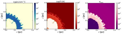
As an illustration, in Fig. 14, we compare the total ionized number density resulting from a simulation for a 1.0–0.569 model without thermal conduction using our usual PN cooling curve with that of a simulation using a cooling curve calibrated for a cooler star (Teff = 40 kK) with standard ISM abundances taken from cloudy (see Table 1), gas density 1 cm−3 and ionizing photon flux ϕ = 109 cm−2 s−1 (Fig. 2, thin-solid line). The appearance of the interface is very different: there are fewer clumps and the instability appears to be more a pure Rayleigh–Taylor type. The density of the clumps at the interface is not large enough to trap the ionizing photons and so the region beyond the swept-up shell is completely photoionized. The differences due to the adopted cooling curves are most important in the temperature range 104 K < T < 106 K. Cooling below 105 K depends on stellar parameters such as effective temperature and ionizing photon rate, while cooling above 105 K is independent of these factors, since the hot gas is collisionally ionized, although the metallicity remains an important ingredient (see Steffen et al. 2012). The cooling curve used in the present simulation is a clear improvement over the standard ISM collisional ionized equilibrium (CIE) cooling curve typically used in hydrodynamical simulations because it uses a more appropriate abundance set and takes into account the ionizing photon flux from the central star, but tailoring the stellar parameters, ionization parameter, and abundance set at each time would be more accurate. A full investigation of this effect is beyond the scope of this work. Finally, our cooling assumes ionization equilibrium but cooling can also be modified if non-equilibrium ionization is taken into account (see Steffen et al. 2008).
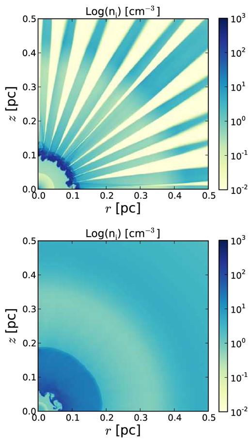
Ionized number density for the 1.0–0.569 model without thermal conduction at 5200 yr. Upper panel: simulation using the PN cooling curve described in Section 2. Lower panel: simulation using a cooling curve for standard ISM abundances, stellar effective temperature Teff = 40 000 K and ionizing flux ϕ = 109 cm−2 s−1 (see Fig. 2).
The clumps and filaments are sources of mixing due to hydrodynamic ablation, shock diffraction and photoevaporation and the large surface area leads to substantial quantities of dense material being shocked and incorporated into the hot bubble. For models without thermal conduction, the breakup of the dense shell can cause hot gas to leak out of the bubble, flowing between the clumps and filaments and thereby depressurizing the hot bubble. The inclusion of thermal conduction leads to evaporation of material at the interface, which fills in the interclump region in the broken shell and reseals the bubble. This results in higher pressures in the conduction models than in those without conduction. Indeed, the expansion of the models without thermal conduction is dominated by the pressure of the thick shell of photoionized gas around the hot bubble, while the models with thermal conduction are more similar to wind-blown bubbles, surrounded by thin shells of swept-up photoionized material.
We have investigated the extent to which numerical diffusion is responsible for mixing across the interface by running a test simulation consisting of an inner, circular region of hot, diffuse gas in pressure equilibrium with a surrounding envelope of dense, cool gas. Both gases were assumed to be at rest, but radiative cooling was taken into account. After 10 000 yr, the interface between the two fluids was only four cells wide and was not growing with time. This gives us confidence that the mixing seen in our simulations without conduction is a real, hydrodynamical effect rather than a numerical one. We have also undertaken studies of the effect of increasing and decreasing the numerical resolution and the size of the wind injection region. The qualitative results are the same, although small details do vary.
5.1 Comparison with previous works
There are some differences that are worth noting between our numerical calculations and the referenced works mentioned in Section 1. We limit our comparison to those works that have taken into account a detailed treatment of the evolution of the stellar wind parameters and show the formation of hot bubbles, principally those studies presented by Villaver et al. (2002a,b), Perinotto et al. (2004), and Steffen et al. (2008).
Potential differences are due to the stellar evolution models, which determine both the initial conditions defined by the final few thermal pulses of the AGB state and the stellar wind parameters in the post-AGB phase, the numerical method and the physics included in the model.
We adopt the same AGB wind parameters as (Villaver et al. 2002a), i.e. those calculated by Vassiliadis & Wood (1993) and so do not expect large departures from their results. Indeed, the density profiles we arrive at at the end of the TP-AGB stage are very similar, particularly the innermost 0.5 pc, which is of most interest to us. We find steep density profiles (ρ ∝ r<−2) for low initial stellar mass models and shallow density profiles (ρ ∝ r>−2) for the high initial stellar mass models. Perinotto et al. (2004) and Steffen et al. (2008) consider two types of AGB winds: a constant mass-loss rate and wind velocity model, which gives a ρ ∝ r−2 density profile, and a ‘hydrodynamical’ model, where the mass-loss rate and wind velocity are based on the AGB mass-loss prescription of Blöcker (1995), which leads to a variable density gradient. As pointed out in these previous works, once the photoionization switches on, the fine details of the initial density and velocity profiles are quickly erased by the shock that passes through the neutral gas ahead of the ionization front.
For the post-AGB evolution, we use the same stellar evolution models as Villaver et al. (2002b). However, we calculate the stellar wind mass-loss and terminal velocity using the wm-basic code (Pauldrach et al. 1986, and subsequent papers.). We also obtained the ionizing photon flux from wm-basic instead of using a blackbody. Our stellar wind parameters differ from those of Villaver et al. (2002b), who use the empirical fits of Vassiliadis & Wood (1994) to the data compiled by Pauldrach et al. (1988). The resulting mass-loss rates are in the same range of values with very similar temporal dependence. On the other hand, the terminal wind velocities obtained by Villaver et al. (2002b) are a factor of approximately 2 higher than ours for all stellar models presented in our Fig. 4 (top-right panel).
Perinotto et al. (2004) and Steffen et al. (2008) use different evolutionary models for the post-AGB stage (Schönberner 1983; Blöcker 1995). Moreover, for stellar effective temperatures below 25 kK, they use the Reimers (1975) prescription for the stellar wind mass-loss rate. Their stellar wind properties are therefore not quite the same as those used in this paper – our mass-loss rates are slightly higher and our wind terminal velocity is slightly lower – but the differences are not significant since the stellar wind mechanical luminosity |$L_\mathrm{w} = 0.5 \dot{M} V_\mathrm{w}^2$| is the important quantity. Once again, a blackbody spectrum is used to calculate the ionizing photon rate.
The minor differences in the stellar wind parameters and ionizing photon rate between our models and previously published work are dynamically not that important. The duration of the transition from the AGB to the WD stage is the main indicator of whether the PN will be density bounded (as seen for the models with initial mass M < 2.5 M⊙) or ionization bounded (as seen for the 3.5–0.754 and 5.0–0.90 models). Our results agree broadly with those of Villaver et al. (2002b) and Perinotto et al. (2004) in this regard but the fact that our simulations are 2D allows the possibility that the shell of AGB material swept up by the fast wind in the early stages of the PN evolution breaks up due to instabilities. For the lower initial stellar mass models, this creates regions of higher opacity (clumps) that may even recombine and become neutral condensations embedded in a surrounding photoionized flow, and regions of lower opacity through which the ionizing photons may pass to photoionize the material beyond the shell. The formation of these clumps starts with the thin-shell instability and depends on the metallicity of the gas and on the form of the cooling curve. The evolution of the photoionized gas within and beyond the shell depends on the radiative transfer model. Our code includes a self-consistent treatment of the radiative transfer and we are able to follow regions of partially ionized, recombining gas (see also Perinotto et al. 2004; Steffen et al. 2008), in contrast to Villaver et al. (2002b) who use the Strömgren approximation.
Unlike Steffen et al. (2008), we find that in our 2D models the thermal conduction does have a dynamical effect on the PN system. For the lower mass CSPN (MWD < 0.677 M⊙), models without conduction have leaky bubbles, whereas thermal conduction reseals the gaps between the clumps and filaments in the broken shell. The gas between the clumps and filaments is material which has been evaporated from the filaments and has expanded as it is heated. The hot bubble in these models grows much more quickly, reaching our ‘target’ distance of 0.2 pc much sooner than in the models without conduction, since there is no loss of pressure, and the interclump material has temperatures T ∼ 105 K. The interclump material in the models without conduction, on the other hand, is hot gas with T > 106 K escaping from the bubble.
Fig. 11 shows that for the higher mass models, the positions of the inner and outer shock waves and the interface between the hot bubble and swept-up shell for models both with and without conduction for the 2D simulations averaged over angle coincide reasonably well with their 1D counterparts. However, in the 2D cases, a substantial amount of dense shell material is shed from the clumps and filaments by hydrodynamic interaction, photoevaporation and thermal evaporation and is thoroughly mixed throughout the hot bubble by non-radial motions. At later times, once the dynamical time has become as large as the cooling time, cooling will become important inside the hot bubble. This will occur much earlier in the 2D simulations than in the 1D simulations because the density is much higher in the former.
While cooling is still unimportant, the effect of thermal conduction is to raise the temperature in the cool, dense gas at the interface with the hot bubble. In both 1D and 2D simulations, the heated gas expands and pushes the swept-up shell outwards. This is particularly the case with the higher mass CSPN models MWD > 0.677 M⊙). These models have larger hot bubbles than their counterparts without conduction, although they still remain enshrouded by neutral material and would not be detectable.
Our 2.5–0.677 model shows intermediate behaviour. The simulation without conduction has ‘leaky bubble’ characteristics, while the simulation with conduction mixes quite a lot of dense shell material back into the bubble. In these models, the clumps in the broken shell recombine and photoevaporated material flows off the heads of these clumps back towards the star.
The effect of thermal conduction on the dynamics is also evident in Fig. 13, where we show the W-shell (dense shell formed by the fast wind–AGB wind interaction) velocity as a function of time for two of our lower mass CSPN models, 1.5–0.597 and 2.0–0.633. For these models, the simulations without conduction are of the ‘leaky bubble’ type, where hot, shocked gas pushes its way between the clumps and filaments of the broken shell. The reduced pressure in the hot bubble results in lower expansion velocities for the external photoionized shell. The corresponding models with conduction remain pressurised, since the gaps in the shell are sealed by material evaporated from the filaments. The expansion velocities in the surrounding photoionized shell are correspondingly higher.
Mellema & Frank (1995) and Mellema (1995) performed 2D axisymmetric radiation-hydrodynamics simulations of the formation of aspherical PNe through an interacting winds model. Their models took into account the density distribution of the circumstellar AGB stage material and although Mellema & Frank (1995) considers constant fast wind parameters, Mellema (1995) takes into account the time evolution of the post-AGB wind and ionizing photons. Unfortunately, the resolution of these simulations is very low (80 × 80 computational cells at best), and although the formation of instabilities at the interface between the hot shocked fast wind and the swept-up photoionized AGB material is hinted at, the numerical resolution is simply not adequate to follow their development. Mellema & Frank (1995) estimate the soft X-ray emission from their models and find it to come from a thin layer just inside the photoionized shell. However, this is an artefact due to numerical diffusion at the contact discontinuity and the low resolution of the simulations converts it into an appreciably amount of soft X-ray emission. Other 2D, purely hydrodynamic simulations by Stute & Sahai (2006) show the formation of instabilities at the contact discontinuity, but these remain confined to a thin layer and do not grow. In our simulations, the resolution is much higher and the instabilities can be characterized and are well developed. Moreover, the strong radiative cooling and the proper treatment of the radiative transfer in our models mean that once the instabilities form they become enhanced and grow in size so that the surface area they present becomes quite large.
We only follow the evolution of our models up until the hot bubble has achieved a radius of ∼0.2 pc. For the 1.0–0.569, 1.5–0.597, and 2.0–0.633 models, this occurs before the mass-loss rate and ionizing photon luminosity have dropped off completely and so it can be expected that these hot bubbles will expand further. The 2.5–0.677 model reaches 0.2 pc only very slowly, since the mass-loss rate and ionizing photon luminosity decline sharply after 3000 yr and it is the residual pressure of the hot bubble that is driving the expansion against the diminishing pressure of the expanding photoionized shell. Our most massive star models, 3.5–0.754 and 5.0–0.90, have such a fast evolution that the hot bubble reaches a maximum radius before the pressure in the hot shocked gas falls below the pressure of the surrounding photoionized shell and the hot bubble collapses back towards the star. This is a natural way of explaining the back-filling of gas in PNe, such as is seen in the Helix nebula (Meaburn et al. 2005; García-Segura et al. 2006).
Finally, we speculate that in the case of 3D simulations the instabilities in the wind–wind interaction zone would develop faster than the formation of clumps in 2D simulations (see Young et al. 2001). This was explored in numerical simulations for the analogous case of the formation of (hot bubbles in) WR nebulae by van Marle & Keppens (2012). They found that 3D simulations show more structure than 2D simulations, although the differences are relatively small. In 3D, there will be a larger surface area of dense AGB material available to be hydrodynamically ablated or evaporated, and we therefore expect that the mixing of material into the hot bubble would be even more effective than in the present 2D results.
6 SUMMARY AND CONCLUSIONS
In this paper, we have presented high-resolution 2D radiation-hydrodynamic numerical simulations of the formation and evolution of hot bubbles in PNe. We considered six different stellar evolution models with initial masses of 1, 1.5, 2, 2.5, 3.5, and 5 M⊙ at solar metallicity (Z = 0.016; Vassiliadis & Wood 1993, 1994), which correspond to final WD masses of 0.569, 0.597, 0.633, 0.677, 0.754, and 0.90 M⊙. The initial circumstellar conditions are obtained from 1D simulations of the final few thermal pulses of the AGB phase and are the same as those used in Villaver et al. (2002a), but in the case of the post-AGB phase the stellar wind velocity, mass-loss rate, and ionizing photon rate are computed self-consistently using the wm-basic stellar atmosphere code (Pauldrach et al. 2012, and references therein). From our results, we find that:
The formation and evolution of hot bubbles in PNe depend on different factors: the density distribution of the previously ejected AGB material, the time evolution of the stellar wind parameters in the post-AGB phase, and the metallicity and cooling rate used in the calculations. Differences between models create different patterns of instabilities in the wind–wind interaction zone. The most important factors are the length of time before the mass-loss rate and ionizing photon rate decline sharply, and the acceleration time-scale for the stellar wind.
The breakup of the shell of swept-up AGB material due to instabilities complicates the wind–wind interaction region and none of our 2D models exhibits a clear double-shell pattern such as those observed by Guerrero, Villaver & Manchado (1998). The formation of clumps leads to dynamic opacity variations in the photoionized shell, which result in bright-rimmed clumps and a ray-like distribution of lower density photoionized gas in the AGB envelope, which vary with time.
The formation and distribution of clumps and filaments have been shown to depend strongly on the cooling rate curve used and the ionization and temperature history of these clumps should be a function of the evolving stellar parameters and radiation field. Although we take into account PN abundances and a representative radiation field when calculating the radiative losses, we do not take into account the time evolution of the stellar parameters nor do we include molecules or dust in our treatment of the neutral gas.
The creation of hydrodynamical instabilities results in mixing of AGB material into the hot bubble, even for cases in which thermal conduction is not included. The temperature and density of the mixing zone are favourable for the emission of soft X-rays.
The inclusion of thermal conduction has several effects: it stops the bubble leaking hot gas through the gaps between the clumps and filaments by sealing them with evaporated material, and it increases the amount of AGB material mixed into the hot bubble. Models without conduction were found to form leaking bubbles with pressures dominated by the photoionized shell, whereas models with conduction resemble wind-blown bubbles surrounded by thin swept-up shells. This changes the appearance of the clumps around the edge of the hot bubble in the two cases. Finally, in cases in which thermal conduction could be suppressed by a magnetic field, hydrodynamical instabilities will dominate the mixing of material into the hot bubble.
The next paper in this series will consider the synthetic X-ray emission (i.e. emission measure, luminosity, surface brightness, and simulated spectra) resulting from these simulations.
We thank the referee, Matthias Steffen, for valuable suggestions that improved the presentation of this paper. We would also like to thank E. Villaver for helpful discussions and for providing the AGB mass-loss rate and velocity parameters of the six stellar evolution models used here. We thank M.A. Guerrero for a critical reading of the manuscript and W. Henney for useful comments. We are grateful to Y. Jiménez-Teja and K. Álamo-Martínez for introducing us to the use of the matplotlib routines. SJA and JAT acknowledge financial support through PAPIIT project IN101713 from DGAPA-UNAM. JAT thanks support by CSIC JAE-Pre student grant 2011-00189.
The temperature in an adiabatically shocked stellar wind is defined by the terminal velocity as |$kT=3 \mu m_{\mathrm{H}} V_{\infty }^{2} /16$|, where k, μ, and mH are the Boltzmann constant, the mean particle mass, and hydrogen mass, respectively.
The most accurate way of doing this would be tailoring the cooling rate to the effective temperature of the central star at each time and the ionizing flux at each position in the nebula, but this procedure would be very time consuming. Nevertheless, Fig. 2 shows that the cooling curves for stars between 50 and 150 kK are very similar.
All 2D images were produced with the matplotlib python routines developed by Hunter (2007).
The obvious difference at small radii is due to the difference in size of the wind injection region in the 2D and 1D cases.
REFERENCES
APPENDIX A: ADDITIONAL FIGURES
In this appendix, we collect together figures for the models not presented in the main text.
Fig. A1 presents final time results for the 1.0–0.569, 2.0–0.638, and 5.0–0.90 models without conduction. For the lower mass models, we define the final time as when the mean radius of the hot bubble reaches 0.2 pc. For the high mass model (5.0–0.90) the final time corresponds to the maximum radius of the hot bubble, after which time it begins to collapse. Fig. A2 presents final time results for the same models with thermal conduction. Models 1.0–0.569 and 2.0–0.638 belong to Group A and exhibit similar behaviour to the 1.5–0.597 model described in the main text. Model 5.0–0.90 is a Group B model and behaves in a similar fashion to the 3.5–0.754 model presented in the main text.
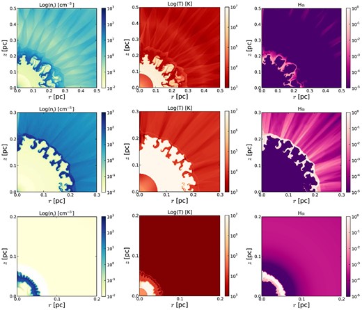
Additional models without conduction. Top row: 1.0–0.569 model at 10 200 yr (when Teff = 31 260 K and L = 3615 L⊙ for this model). Middle row: 2.0–0.633 model at 4200 yr (when Teff = 171 790 K and L = 3200 L⊙ for this model). Bottom row: 5.0–0.90 model at 770 yr (when Teff = 213 800 K and L = 400 L⊙ for this model). The first and second rows correspond to the hot bubble having a mean radius of 0.2 pc. The third row corresponds to the maximum radius of the hot bubble for the 5.0–0.90 model. From left to right, the panels represent: total ionized number density (left-hand panels), temperature (middle panels), and normalized Hα volume emissivity (right-hand panels).
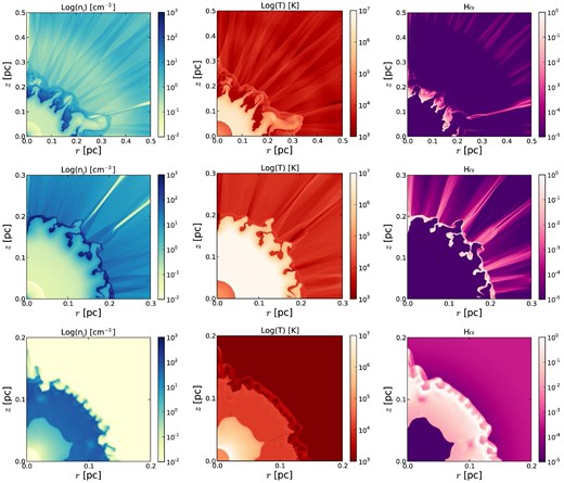
Additional models with thermal conduction. Top row: 1.0–0.569 model at 8700 yr (when Teff = 29 040 K and L = 3622 L⊙ for this model). Middle row: 2.0–0.633 model at 3600 yr (when Teff = 159 220 K and L = 4520 L⊙ for this model). Bottom row: 5.0–0.90 model at 3370 yr (when Teff = 180 720 K and L = 180 L⊙ for this model). The first and second rows correspond to the hot bubble having a mean radius of 0.2 pc. The third row corresponds to the maximum radius of the hot bubble for the 5.0–0.90 model. From left to right, the panels represent: total ionized number density (left-hand panels), temperature (middle panels), and normalized Hα volume emissivity (right-hand panels).
