


Abstract
Heavily obscured and Compton-thick active galactic nuclei (AGNs) are missing even in the deepest X-ray surveys, and indirect methods are required to detect them. Here we use a combination of the XMM–Newton serendipitous X-ray survey with the optical Sloan Digital Sky Survey (SDSS), and the infrared WISE all-sky survey in order to check the efficiency of the low X-ray-to-infrared luminosity selection method in finding heavily obscured AGNs. We select the sources which are detected in the hard X-ray band (2–8 keV), and also have a redshift determination (photometric or spectroscopic) in the SDSS catalogue. We match this sample with the WISE catalogue, and fit the spectral energy distributions of the 2844 sources which have three, or more, photometric data points in the infrared. We then select the heavily obscured AGN candidates by comparing their 12 μm luminosity to the observed 2–10 keV X-ray luminosity and the intrinsic relation between the X-ray and the mid-infrared luminosities. With this approach, we find 20 candidate heavily obscured AGNs and we then examine their X-ray and optical spectra. Of the 20 initial candidates, we find nine (64 per cent; out of the 14, for which X-ray spectra could be fitted) based on the X-ray spectra, and seven (78 per cent; out of the nine detected spectroscopically in the SDSS) based on the [O iii] line fluxes. Combining all criteria, we determine the final number of heavily obscured AGNs to be 12–19, and the number of Compton-thick AGNs to be 2–5, showing that the method is reliable in finding obscured AGNs, but not Compton thick. However, those numbers are smaller than what would be expected from X-ray background population synthesis models, which demonstrates how the optical–infrared selection and the scatter of the Lx-LMIR relation limit the efficiency of the method. Finally, we test popular obscured AGN selection methods based on mid-infrared colours, and find that the probability of an AGN to be selected by its mid-infrared colours increases with the X-ray luminosity. The (observed) X-ray luminosities of heavily obscured AGNs are relatively low (|$L_{\rm 2{\rm -}10\,keV}<10^{44}\,{\rm erg\,s^{-1}}$|), even though most of them are located in the ‘quasi stellar object (QSO) locus’. However, a selection scheme based on a relatively low X-ray luminosity and mid-infrared colours characteristic of QSOs would not select ∼25 per cent of the heavily obscured AGNs of our sample.
INTRODUCTION
Supermassive black holes (SMBHs) are considered to be one of the major building blocks of the Universe. Most nearby galaxies are seen to harbour an SMBH (e.g. Kormendy 1987; Ishisaki et al. 1996; Matt et al. 1996b), including the Milky Way (Genzel, Eisenhauer & Gillessen 2010), and it is found that the mass of the SMBH is tightly connected to properties of the bulge of the galaxy (e.g. Ferrarese & Merritt 2000; Gebhardt et al. 2000). The growth of a black hole to reach a mass of ≳106 M⊙ must include a phase of rapid accretion, i.e. an active galactic nucleus (AGN; Rees 1984), unless it forms from an already massive primordial black hole (see Volonteri 2012). This has implications for the formation and growth of galaxies and other structures in the Universe (see also Alexander & Hickox 2012; Fabian 2012); therefore, a complete census of AGNs in the Universe is essential in order to study its evolution.
The most efficient way to detect an AGN is through its high-energy emission detected in the X-rays. The deepest X-ray surveys with Chandra and XMM–Newton (Alexander et al. 2003; Brunner et al. 2008; Xue et al. 2011; Ranalli et al. 2013) have detected a large number of AGNs, with a surface density tens of times higher than that found in optical surveys (Bauer et al. 2004; Xue et al. 2011). A representative sample of AGNs in the Universe over different scales and redshifts can be drawn by combining deep pencil-beam surveys with wider, intermediate-depth surveys (e.g. Cappelluti et al. 2009; Elvis et al. 2009) and shallow large-area surveys (e.g. Voges et al. 2000; Watson et al. 2009). Most of the AGNs detected in the X-rays show some level of obscuration (Hasinger 2008), but the hard X-rays (2–10 keV) can easily penetrate large columns of obscuring material in the cases where the dominant X-ray absorption mechanism is photoelectric absorption, because of the strong dependence of its cross-section on the photon energy (σPE ∝ E−3). However, when the column density of the obscuring material reaches NH ≈ 1.5 × 1024 cm−2 (i.e. the inverse of the Thomson cross-section for electrons, |$\sigma _{\rm T}^{-1}$|), it becomes optically thick to Compton scattering, the relativistic equivalent of Thomson scattering applied at higher energies, which has a lower dependence on energy. Such sources are called Compton-thick (CT) AGNs and even high-energy photons are obscured. If the column density is NH ≲ 5 × 1024 cm−2, we can still detect some X-ray photons from the source, with a hard spectrum peaking at ∼10 keV, where the Compton and photoelectric cross-sections are equal (transmission-dominated CT AGNs). If the column density is even higher, any detected X-ray emission comes from a reflected component at the back side of the obscuring torus (reflection-dominated CT AGNs; e.g. Matt, Brandt & Fabian 1996a), giving a characteristic flat X-ray spectrum, with an observed luminosity typically a few per cent of the intrinsic AGN luminosity (e.g. Maiolino et al. 1998; Matt et al. 2000). In some cases, a soft (Γ > 1.8) component scattered possibly from electrons in the narrow-line region is also detected in lower X-ray energies (≲2 keV; see e.g. Netzer, Turner & George 1998), which is a blend of photoionized lines (Guainazzi & Bianchi 2007).
The fact that the observed X-ray emission from CT AGNs is only a fraction of the intrinsic emission, even at the highest energies detected by X-ray telescopes, makes them challenging to detect in even the deepest X-ray surveys. Therefore, other techniques have been developed, which use the combination of a low detected X-ray luminosity (or even a non-detection) with secondary processes taking place in the AGNs. The most widely used methods employ optical (or near-infrared) spectroscopy focusing on high-excitation spectral lines coming from the narrow-line region (e.g. Bassani et al. 1999; Cappi et al. 2006; Akylas & Georgantopoulos 2009; Gilli et al. 2010; Vignali et al. 2010; Mignoli et al. 2013), and mid-infrared photometry tracing the reprocessed dust emission from the absorbing material (e.g. Daddi et al. 2007; Fiore et al. 2008, 2009; Alexander et al. 2011). The spectral line technique is observationally challenging, as it requires relative bright sources in the optical wavelengths. It has been mostly used in narrow fields utilizing multislit spectroscopy (Juneau et al. 2011), or to a limited number of sources in wide fields (e.g. Cappi et al. 2006). In this paper, we will use the mid-infrared emission, which is easier to apply to wide fields.
The mid-infrared emission from the AGNs is due to the obscuring dust heated by the AGN X-ray and ultraviolet emission. However, dust is also abundantly found around massive O–B stars in the host galaxies, and is heated by their ultraviolet radiation, making infrared emission also a star formation tracer (e.g. Calzetti et al. 2010). In order to differentiate between the two different generators of infrared emission, we must take into account the high energy produced by the AGNs, which heats the dust to higher temperatures than O–B stars and gives a characteristic power-law spectrum in the mid-infrared (Neugebauer et al. 1979) and peaks at ∼ 10–20 μm (see Nenkova et al. 2008; Stalevski et al. 2012 for models involving clumpy tori). This feature is used to select AGNs based on their mid-infrared colours (e.g. Stern et al. 2005; Donley et al. 2012; Mateos et al. 2012, 2013) or power-law shape of the spectral energy distribution (SED; e.g. Alonso-Herrero et al. 2006; Donley et al. 2007). The peak of the AGN-powered IR emission at ∼ 10–20 μm also coincides with the minimum of the host SED at these wavelengths (see e.g. Chary & Elbaz 2001), which makes a direct mid-infrared selection possible. This has been extensively used to select obscured AGNs in medium-to-deep surveys (Georgantopoulos et al. 2011, and references therein) by their low X-ray-to-infrared luminosity ratio, utilizing the empirical intrinsic Lx/LMIR relation (Lutz et al. 2004; Gandhi et al. 2009; Asmus et al. 2011).
The low Lx/LMIR selection technique has not been widely used in broad surveys, because of the lack of MIR observations covering a large part of the sky. Before the advent of WISE (Wright et al. 2010), the only all-sky survey products in the mid-infrared were the AKARI survey, and the IRAS point source catalogue (Beichman et al. 1988), which is used by Severgnini, Caccianiga & Della Ceca (2012), giving promising results. In this work, we will use the recently publicly available results from the WISE all-sky survey, in conjunction with the wide-field XMM–Sloan Digital Sky Survey (SDSS) catalogue (Georgakakis & Nandra 2011) to perform a wide search for X-ray detected CT AGNs. We will also use a new SED decomposition technique to isolate the mid-infrared emission from the AGNs and thus minimize the host galaxy contamination. We will then test the efficiency of the low X-ray-to-mid-infrared luminosity method by examining the X-ray and optical spectral properties of the candidate sources, and comparing their number with that expected from X-ray background synthesis models. We adopt H0 = 71 km s−1 Mpc−1, ΩM = 0.27 and ΩΛ = 0.73 throughout the paper.
DATA
X-ray catalogue
We use the X-ray catalogue compiled by Georgakakis & Nandra (2011), which contains about 40 000 X-ray point sources over an area of 122 deg2, with a half-area detection limit of 1.5 × 10⁻¹⁴ erg s−1 cm−2 in the 0.5–10 keV band and 3 × 10⁻¹⁴ erg s−1 cm−2 in the 2–10 keV band. This survey uses XMM–Newton pointings which coincide with the SDSS DR7 (Abazajan et al. 2009), and we use it in order to have optical and near-infrared photometric information, as well as a spectroscopic or photometric redshift for our candidates. The source detection has been performed by Georgakakis & Nandra (2011) straight from the XMM–Newton observations without using the automated source extraction of Watson et al. (2009). All XMM–Newton observations performed prior to 2009 July, overlapping with the SDSS, have been used in the analysis, and X-ray photometry is provided in five bands, including the 0.5–2.0 and 2–8 keV, hereafter ‘soft’ and ‘hard’ bands, respectively, that we investigate here.
Infrared
For the (mid-)infrared identification of our candidates, we use the all-sky source catalogue of WISE (Wright et al. 2010). This is a space telescope launched in 2009 December, operating in the mid-infrared part of the spectrum. It has a 40 cm primary mirror and performed an all-sky survey in the 3.4, 4.6, 12 and 22 μm bands, reaching 5σ point source sensitivities of 0.08, 0.11, 1 and 6 mJy, or lower, depending on the position in the sky. The full width at half-maximum (FWHM) of the point spread functions (PSFs) are 6.1, 6.4, 6.5 and 12.0 arcsec for the four bands, respectively, which are comparable to that of XMM–Newton (≈5–10 arcsec, depending on the instrument and off-axis angle), allowing us to perform a reliable search for counterparts between the two telescopes. We use the magnitudes measured with profile-fitting photometry and the zero-points of Jarrett et al. (2011).
THE SAMPLE
The X-ray sample of Georgakakis & Nandra (2011) contains 39 830 X-ray sources within the footprint of the SDSS DR7 survey. Georgakakis & Nandra (2011) use the likelihood ratio method1 to find optical counterparts for the X-ray sources. At a limit of LR = 1.5, they find a counterpart for almost half of X-ray sources (19 431/39 830) with an expected spurious identification rate of 7 per cent. The probability that an X-ray source has an optical counterpart is strongly dependent on the X-ray flux, and is typically ≈50 per cent for sources with |$f_{\rm 0.5{\rm -}10\,keV}\approx 2\times 10^{-14}\,{\rm erg\,s^{-1}\,cm^{-2}}$| and ≈90 per cent for sources with |$f_{\rm 0.5{\rm -}10\,keV}\approx 2\times 10^{-13}\,{\rm erg\,s^{-1}\,cm^{-2}}$| (Georgakakis & Nandra 2011). A redshift determination requires a spectroscopic follow-up in the optical (or the near-infrared) and a good enough quality spectrum, which is the case for the brightest optical sources (typically with r < 17.77). We note that in addition to SDSS spectroscopy, a number of optical spectroscopic programmes were used in Georgakakis & Nandra (2011), so there are sources with optical spectra with magnitudes exceeding the r = 17.77 limit, but not with uniform coverage in terms of spatial distribution, or source type. In addition to spectroscopic redshifts, a source might have a photometric redshift determination, if it is detected in enough optical and near-infrared bands. The typical detection limits for the SDSS DR7 are r < 22.2 and z < 20.5. Only half of the SDSS detected X-ray sources have a redshift determination (9029/19 431), 2172 of them being spectroscopic.
In identifying heavily obscured sources by their low X-ray-to-infrared ratio, it is possible that the sample will be contaminated by a number of normal galaxies, i.e. X-ray sources that do not host an AGN, and their X-ray flux is attributed to star formation. The normalization of the X-ray-to-infrared relation for star-forming galaxies (e.g. Ranalli, Comastri & Setti 2003) is one to two orders of magnitude lower than the X-ray-to-infrared ratio of typical AGNs (see Section 5.3), so normal galaxies could be mistaken for highly obscured AGNs. To minimize this effect, we limit our X-ray sample to those X-ray sources that are detected in the hard band (2–8 keV), so that we are able to have an initial hint of the shape of the X-ray spectrum through the hardness ratio, without having to analyse all the spectra prior to the candidate selection. 4553/9029 X-ray sources with a redshift determination are detected in the hard band.
Looking for WISE counterparts
We look for counterparts to the 4553 X-ray sources described in the previous section in the WISE all-sky catalogue. Because at the flux limits of both XMM–Newton and WISE the confusion of the sources is minimal (within 5 arcsec of the X-ray positions there are 4100 WISE counterparts with seven duplicates), we use a simple proximity criterion to select the counterparts (see e.g. Rovilos et al. 2009). In order to have an estimate of the number of spurious counterparts, we initially select sources from the WISE catalogue that are within 60 arcsec of the X-ray positions. In Fig. 1, we plot the histograms of the difference in RA and Dec. of the counterparts, and in red we plot Gaussians fitted to the distributions. We find a mean dRA = 0.73 ± 2.42 arcsec and dDec. = −0.57 ± 1.95 arcsec, which are consistent with the astrometric accuracies of the XMM–Newton catalogue (1–2 arcsec; see Watson et al. 2009; Georgakakis & Nandra 2011). The nominal astrometric accuracy of the WISE all-sky catalogue is ∼0.3 arcsec at the faintest fluxes. We correct the positional differences between the sources of the two catalogues by the above mean values.
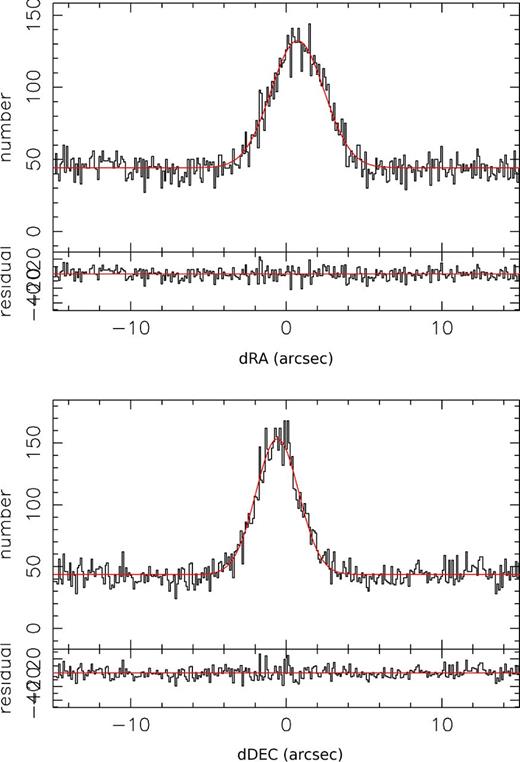
Histograms of the differences between the RA and Dec. values of the XMM–Newton and WISE sources. Both distributions are fitted with Gaussians (red lines), where the mean and standard deviation values quoted in Section 3.1 are derived from. We detect an ∼0.7 arcsec and ∼0.6 arcsec shift in RA and Dec. respectively, and we correct the matching coordinates accordingly. (The colour figure is available in the online version.)
Next, we estimate the number of spurious counterpart matches. Given the distributions of Fig. 1 and the Gaussian fits, we can assume that most of the counterparts with dRA and dDec. greater than 6 arcsec (≈2σ) are chance matches. In order not to include any real counterparts when assessing the spurious ratio, we measure the number of matches with distances of 20–40 arcsec, and find 14 861 cases. Therefore, the density of spurious counterparts in the dRA–dDec. space is 3.9 arcsec−2. In Fig. 2, we plot the histogram of the distances of all the counterparts. We model this with a Rayleigh distribution with an amplitude set to be the mean of the amplitudes of the two Gaussian distributions and parameter |$\sigma ^{2}=(\sigma _{\rm RA}^{2}+\sigma _{\rm Dec.}^{2})/2$| (dotted line). We also add the expected number of spurious counterparts calculated above (dashed line). The sum of those two distributions is plotted with the solid curve in Fig. 2. We overpredict the number of counterparts with distances 5–12 arcsec, and we attribute this difference to the finite PSF of the WISE survey: if there is a WISE source detected close to the position of the X-ray source (being the ‘true’ counterpart), another detection is unlikely in its immediate vicinity (5–12 arcsec), which would be the spurious counterpart, because of the blending of their PSFs. The two sources would become distinguishable if their distance is more than two times the FWHM of the PSF and in WISE this is 12 arcsec. With the green histogram in Fig. 2, we plot the distribution of unique counterparts, choosing the nearest case, and this is almost identical with the black histogram below 5 arcsec. The two distributions (Rayleigh of ‘correct’ counterparts and linear of spurious) meet at 4.3 arcsec, and choosing a limiting radius larger than that would give more chance matches than true counterparts. Since in this study we are searching for a rare type of object (given the high flux density limits), we are more conservative and use 3.5 arcsec as our limiting radius, indicated by the grey area in Fig. 2. Within this radius, we find 3689 (3685 unique) matches between the XMM–Newton and WISE catalogues, and the number of spurious counterparts expected within this radius is 150 (4.1 per cent). We do not find a WISE counterpart for 868 sources, something that might introduce a bias in the selection of obscured AGNs (see Section 6.2). However, such cases have by definition high X-ray-to-mid-infrared luminosity ratios and would not be selected as candidates, even if the infrared lower limits were such that they would be detected.
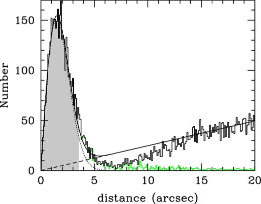
Histogram of the distances between matched sources from the XMM–Newton and WISE catalogues. The dotted curve shows a Rayleigh distribution calculated from the Gaussian fits of Fig. 1, and the dashed line shows the expected distribution of spurious counterparts, constant in the dRA–dDec. parameter space. The solid curve denotes their sum, which is a good representation of the observed histogram, except for the 5–12 arcsec region due to the WISE PSF (see Section 3.1). The shaded area represents the 3.5 arcsec threshold used in this study, and the green line shows the histogram of the distribution of unique counterparts. (The colour figure is available in the online version.)
CANDIDATE OBSCURED SOURCES
We select our sample of candidate heavily obscured AGNs based on the X-ray-to-mid-infrared rest-frame luminosity ratio. Gandhi et al. (2009), exploring the nuclear X-ray (2−10 keV) and mid-infrared (12.3 μm) properties of a sample of nearby Seyferts, found a correlation between their rest-frame luminosities, when correcting the X-ray fluxes for internal absorption and using high angular resolution in the mid-infrared to resolve out the host emission (see also Asmus et al. 2011). This correlation is thought to be characteristic of AGNs, and any deviations from it (in the form of an infrared excess) should arise from severe obscuration of the X-ray photons. This assumption has been used in the past to select heavily obscured AGNs (e.g. Alexander et al. 2008; Goulding et al. 2011), and although the samples acquired are not complete, they are reliable (see also Georgantopoulos et al. 2011) in the sense that the majority of selected sources have indications of being heavily obscured, especially in the local Universe. However, as shown by Georgakakis et al. (2010) and Asmus et al. (2011), the host galaxy is a contaminant of the mid-infrared flux, which affects relatively low-luminosity AGNs; these can be mistaken for obscured AGNs, whereas in reality they are ‘low AGN-to-host infrared sources’. To avoid such cases, we decompose the infrared SEDs of the sources in our sample, as explained below.
SED decomposition
For the X-ray luminosities, we use the 2–10 keV fluxes from the catalogue of Georgakakis & Nandra (2011) and a photon index Γ = 1.4 for the k-corrections to obtain rest-frame 2–10 keV luminosities. Although the detection band is 2–8 keV, the fluxes are for the 2–10 keV band and are calculated from the photon counts of all three detectors of XMM–Newton, after carefully modelling and subtracting the background (see Georgakakis & Nandra 2011 for more details). To calculate the mid-infrared luminosities, we use all the near- and mid-infrared information provided by WISE: the photometry in the four WISE bands (3.4, 4.6, 12 and 22 μm), as well as the photometry in the three 2MASS bands (J, H and K) for detected sources. The WISE catalogue provides near-infrared (JHK) photometry for sources with a counterpart in the 2MASS point source catalogue, based on the best matching 2MASS source. However, some of the low-redshift sources are extended and their near-infrared counterparts are in the 2MASS extended source catalogue, which is not taken into account. Therefore, we look for counterparts of the XMM–WISE sources in the 2MASS extended source catalogue and find 321 counterparts within 3 arcsec of the WISE positions. For those cases, we correct the near-infrared photometry.
In this study, we are interested in the mid-infrared luminosity from the AGNs and the host galaxy is a potential contaminant that cannot be resolved by WISE; we decompose the infrared SED into an AGN and a galaxy component. We use a custom-built maximum likelihood method to find an optimum combination of a semi-empirical galaxy template from Chary & Elbaz (2001), with an AGN template of Silva, Maiolino & Granato (2004), and measure the 12 μm monochromatic luminosity (νLν(12 μm)) from the AGN template. We do this to sources with a photometric detection in at least three of the J, H, K, 3.4 μm, 4.6 μm, 12 μm, 22 μm bands, since we use the combination of two templates, and this selection limits the number of sources from 3685 to 2844. We combine the photometric errors given in the WISE (and/or the 2MASS extended) catalogue with a 10 per cent-level error of the photometric value in quadrature, to account for the intrinsic error on the SED templates used. The different criteria that were used to select these 2844 sources whose SEDs are fitted from the 39 830 X-ray sources in the XMM–SDSS catalogue are summarized in Table 1.
Selections made to the initial X-ray source sample.
| Selection | Number of residual sources |
|---|---|
| Initial | 39 830 |
| SDSS counterpart | 19 431 |
| Redshift determination | 9029 |
| Hard X-ray detection | 4553 |
| WISE counterpart | 3685 |
| SED fit (≥3 WISE–2MASS bands) | 2844 |
| Selection | Number of residual sources |
|---|---|
| Initial | 39 830 |
| SDSS counterpart | 19 431 |
| Redshift determination | 9029 |
| Hard X-ray detection | 4553 |
| WISE counterpart | 3685 |
| SED fit (≥3 WISE–2MASS bands) | 2844 |
When trying to decompose the SEDs using multiple components and a limited number of data points, we are expecting degeneracies between the different fitted components. Therefore, in order to have an estimate of the uncertainty of the νLν(12 μm) value calculated, for every trial fit we plot the 12 μm flux of the AGN template against the (log) likelihood referring to it in the left-hand panels of Fig. 3. An example of reliable and unreliable estimates of νLν(12 μm), as well as the SED combination with the highest likelihood, is shown in Fig. 3: the right-hand panels show the composite best-fitting SED with the grey line, using the combination of the galaxy (red) and AGN (blue) templates that give the maximum likelihood value. In this case, we do not use any priors in the maximum likelihood estimation, so the difference in the natural logarithms of the likelihoods is equivalent to the difference in χ2 of the fits. With the dashed lines in the left plots, we indicate the χ2 differences from the best fit corresponding to 68.3, 95.4 and 99.7 per cent (or 1σ, 2σ and 3σ) confidence levels. In order to check whether the AGN template is indeed needed, we plot the likelihood values of a single-template fit using only the host template in the far-left column of the likelihood plots. For the cases shown in Fig. 3, this is visible only in the lower panel, where the likelihood values are comparable to the ones of the fits involving two templates. In this case, it indicates that a solution with no AGN template is almost as likely as the best solution involving the combination of two templates; therefore, the AGN template is not statistically important assuming a 2σ confidence level; its significance is slightly higher than 1σ according to Fig. 3. The SED decomposition procedure is explained in more detail in Appendix A.
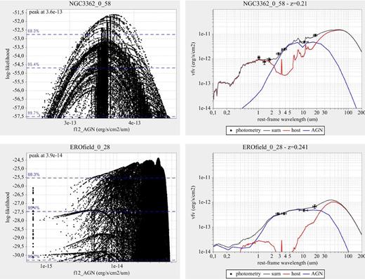
Examples of a well-defined value of monochromatic AGN 12 μm luminosity (top panel), and one where only an upper limit can be defined, so that an AGN component is not required for the SED fitting (bottom panel). In the left-hand panels, we plot the AGN monochromatic flux density against the log-likelihoods of all the trial fits involved in finding the best-fitting solutions plotted in the right-hand panels. In the right-hand panels, the red lines denote the host templates that give the best overall fit, the blue lines the AGN templates and the grey lines their combinations. (The colour figure is available in the online version.)
Identifying heavily obscured AGN candidates
In Fig. 4, we plot the 2–10 keV X-ray luminosity against the 12 μm monochromatic luminosity of the AGN component. The grey area represents the relation expected from Gandhi et al. (2009) (±log (3), corresponding to σ ≈ 0.5 dex). The hardness provides an initial indication of the obscuration of the sources, and we plot the soft and hard sources in blue and red colours, respectively, taking a hardness ratio (|${\rm HR}=\frac{H-S}{H+S}$|, where H and S are the count rates in the hard and soft bands, respectively) threshold of HR = −0.35, which corresponds to Γ = 1.4 (see also Mainieri et al. 2007). Using this threshold, 38 per cent of the fitted sources (1089/2844) are obscured. In light blue and red symbols, we plot sources where the infrared AGN component is not detected with a significance above 2σ, and in the black data point on the top-left of the image we indicate the median 95 per cent uncertainty of the intrinsic 12 μm luminosity. The error on the X-ray luminosity coming from the count rate is too small to be plotted in this diagram; however, there is an uncertainty on the X-ray flux rising from the shape of the X-ray spectrum, which can be substantial, but detailed a priori knowledge is impossible. We correct for this factor for the sources whose spectra we fit, and we note here that it can be a source of the scatter we observe in Fig. 4, especially since we are plotting observed values, not corrected for absorption. We observe a shift of 0.08 dex between the mean values of |$L_{\rm 2{\rm -}10\,keV}/\nu L_{\rm \nu (12\,\mu \mathrm{m})}$| of X-ray obscured and unobscured sources, but given that the scatter in both cases is 0.5 dex, we do not consider the shift to be important. We observe an overall average shift of a factor of ∼2 between the position of the data points and the Gandhi et al. (2009) relation, which could be attributed to an absorbing column of ∼1023 cm−2, or some residual contribution of the host galaxy to the derived AGN infrared luminosity. There is evidence however that the X-ray-to-mid-infrared relation at higher redshifts deviates from the local relation of Gandhi et al. (2009), but we should consider that the points plotted here correspond to the cases where a contribution to the mid-infrared flux from the AGNs is detected by the SED fitting, and this is the case for 2617 out of the 2844 sources fitted, half of them (1313) being upper limits within 2σ. The average |$L_{\rm 2{\rm -}10\,keV}/\nu L_{\rm \nu (12\,\mu \mathrm{m})}$| ratios therefore are biased towards lower values, and we cannot draw safe conclusions on any significant deviation from the Gandhi et al. (2009) relation.
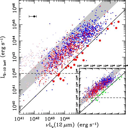
Hard X-ray (2–10 keV) luminosities plotted against the 12 μm monochromatic luminosities of the AGN component for soft (blue; HR < −0.35) and hard (red; HR ≥ −0.35) X-ray sources. In light blue and red symbols are plotted the cases where the significance of the torus component is below 2σ (95 per cent). The black point on the top left of the diagram shows the median 95 per cent uncertainty of the intrinsic 12 μm luminosity as a representative error bar. The expected relation from Gandhi et al. (2009) (±log (3)) is shown by the grey area. The selection line (solid line) for our heavily obscured candidates represents a 4 per cent reflection component from the obscured AGNs, and the candidates are represented with the large red symbols. The dashed line represents the limit of Lx = 1042 erg s−1, below that the host galaxy contamination in the X-rays cannot be considered negligible. In the inset image, we plot the same values but with the 2σ lower limit of the mid-infrared luminosity in the x-axis. The candidates are plotted with green colour, and half of them are below the black solid line. (The colour figure is available in the online version.)
In order to find the most heavily obscured X-ray sources, we search for sources that significantly deviate from the bulk of the X-ray–mid-infrared correlation. In heavily obscured sources, only a fraction of the direct X-ray emission from the AGNs is detectable, and especially in CT sources, all we detect are the X-ray photons reflected at the back side of the torus, or scattered by it; the intensity of this reflection/scattered component is typically a few per cent of the X-ray energy output of the AGNs at 2–8 keV energies (see Matt et al. 2000; Risaliti & Elvis 2004). The solid line in Fig. 4 represents the X-ray–mid-infrared correlation shifted by a factor of 25 in the X-rays, and we will use this to select the heavily obscured candidates for this paper. There are 42 sources (out of the 2844 whose infrared SED is fitted) lying below the solid line of Fig. 4.
If we consider local CT AGNs where the X-ray luminosity is dominated by the nucleus, they are in general hard X-ray sources. Here we give the examples of Mrk 3 (Griffiths et al. 1998), NGC 4945 (Yaqoob 2012), NGC 7582 (Schachter et al. 1998), NGC 6240 (Iwasawa & Comastri 1998; Komossa et al. 2003), NGC 424 (Marinucci et al. 2011) and ESO 565–G019 (Gandhi et al. 2013). Their observed X-ray emission comes predominantly from a (flat) reflection component and a photoionized scattered component, which in general has a soft spectrum. However, in most cases the reflected component seems to dominate. In some cases, a star formation X-ray component is also present (see La Massa, Heckman & Ptak 2012). However, the hardness ratios of these CT AGNs in the XMM–Newton bands used in this paper would all be >+0.4. See Comastri (2004) and Della Ceca et al. (2008) for a more complete list of nearby CT X-ray AGNs. A notable exception is NGC 1068, which has a steep X-ray spectrum below ∼2 keV and a flat spectrum at higher energies (Elvis & Lawrence 1988), with the lower energy components being dominant, so that its hardness ratio in the XMM–Newton bands used here is HR ≈ −0.45. As revealed by high-resolution (grating) X-ray spectroscopy, the soft X-ray component of NGC 1068 is a blend of recombination lines coming from photoionized regions (Brinkman et al. 2002; Kinkhabwala et al. 2002), hence intrinsic in the nuclear region, which dominates in the X-rays, despite the fact that the nuclear region of NGC 1068 is a vigorously star-forming region (e.g. Thronson et al. 1989; Davies, Sugai & Ward 1998).
Since the reflection component of the AGN is usually flat with Γ ∼ 1 (see also George & Fabian 1991), we exclude sources with HR < −0.35, which corresponds to Γ > 1.4 reducing the sample to 22 sources. Our final sample of heavily obscured candidates contains 20 sources, which are plotted with large red symbols in Fig. 4, and lie below the black solid line. For two of the 22 initial candidates, the torus contribution to the infrared SED is not significant at the 2σ level, according to the SED decomposition described in the previous section. In the inset plot of Fig. 4, we plot the 2σ lower limits of the torus 12 μm luminosities on the x-axis. The 20 candidate sources are plotted in green colour, and we can see that 10 of them are still below the black solid line. These sources are underluminous in the X-rays with respect to their mid-infrared luminosities even when their mid-infrared lower limits are considered, and form the most reliable half of the candidate sample.
For the 20 candidate heavily obscured sources, we search for the correct counterparts in the 2MASS and SDSS catalogues and also for a far-infrared detection in the IRAS catalogue, and perform the SED fitting again, this time also including the optical (ugriz) data points and a separate stellar component. For the latter, we use the stellar population synthesis models of Bruzual & Charlot (2003), reddened with the reddening law described in Calzetti et al. (2000). We use solar metallicity and a varying age and star formation history to find the optimum template for each source, and using the best-fitting template gives an estimate of the stellar mass of the source. However, some sources in our sample have a point-like morphology, which indicates that the AGN dominates over the optical flux. For such cases, we use AGN templates from the SWIRE template library (Polletta et al. 2007), which have a prominent blue component, and introduce a Bayesian prior for the maximum likelihood fit. Indeed, in the best-fitting solutions, we see that the AGN template dominates the SDSS bands. For the far-infrared (star formation) part of the SED, we use the templates of Mullaney et al. (2011), which have a better representation of the polycyclic aromatic hydrocarbon features than those of Chary & Elbaz (2001). The new SED fitting confirms that the torus component is statistically important for all 20 sources and that they are underluminous in the X-rays compared to that predicted from their best-fitting torus mid-infrared luminosities and the relation of Gandhi et al. (2009). We also fit a random subsample (450) of the overall sample of the 2844 sources using the three-template approach including the optical bands, and find that their AGN mid-infrared luminosities are similar to that measured using the two-component approach; 85 per cent are within the 95 per cent νLν(12 μm) uncertainty plotted in Fig. 4. This happens because the extra (optical) data are fitted using the extra (stellar or blue bump) component, without having a major effect on the infrared fit.
The basic properties of the heavily obscured AGN candidates are shown in Table 2, where in the last column we indicate the number of infrared data points used. We note that most sources have seven points, but there are six sources for which only four infrared data points can reveal the presence of an AGN. This shows the power of the mid-infrared band in selecting AGNs, and happens because of the seemingly different shape of the hot dust SED to that of a typical host at those wavelengths. The redshift distribution is shown in Fig. 5 with red and purple points, the red points marking the most reliable outliers. With filled circles we mark the observed X-ray luminosities, and with open circles the intrinsic luminosity derived from the infrared luminosity and the relation of Gandhi et al. (2009). The grey crosses represent all the X-ray sources for which an infrared SED is fitted; we note that the intrinsic luminosities are significantly higher than the mean luminosities of the X-ray sample, and this is what is expected for a sample of heavily obscured AGNs, yet still observed in the X-rays.
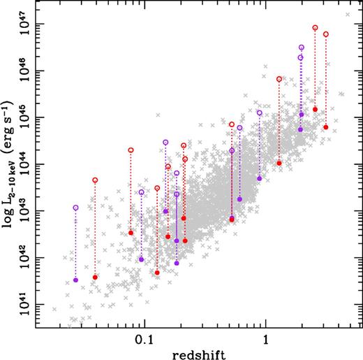
The redshift distribution of the heavily obscured candidate sources plotted with red and purple points, the red points marking the most reliable outliers. In solid circles, we plot the observed X-ray luminosity and in open circles the intrinsic X-ray luminosity inferred from the mid-infrared luminosity of each source. In grey crosses are plotted all X-ray sources for which an infrared SED is fitted. (The colour figure is available in the online version.)
Basic properties of the CT candidate sources.
| Number | Name | log νLν(12 μm)AGN | log νLν(12 μm)AGN, lim | |$\log L_{\rm 2{\rm -}10\,keV}$| | |$\log L_{\rm 2{\rm -}10\,keV}^{\rm MIR}$| | z | [3.4] − [4.6] | AGN | HR | Nphot |
|---|---|---|---|---|---|---|---|---|---|---|
| (1) | (2) | (3) | (4) | (5) | (6) | (7) | (8) | (9) | (10) | (11) |
| 1 | J073502.30+265911.6 | 47.08 | 46.87 | 45.06 | 46.50 | 1.973 | 1.251 | 97 per cent | −0.24 | (7) |
| 2 | J075820.97+392336.0 | 44.42 | 44.05 | 42.36 | 44.11 | 0.216 | 1.580 | 43 per cent | −0.13 | (7) ✓ |
| 3 | J082501.49+300257.3 | 45.52 | 45.35 | 43.69 | 45.10 | 0.888 | 1.530 | 56 per cent | +0.20 | (4) |
| 4 | J090959.59+542340.5 | 44.62 | 44.46 | 42.85 | 44.29 | 0.526 | 1.173 | 42 per cent | +0.04 | (4) |
| 5 | J091848.61+211717.1 | 44.82 | 44.73 | 42.99 | 44.47 | 0.149 | 1.034 | 99 per cent | −0.22 | (7) |
| 6 | J093551.60+612111.8 | 43.92 | 43.75 | 41.58 | 43.66 | 0.039 | 1.688 | 40 per cent | −0.15 | (7) ✓ |
| 7 | J093857.01+412821.1 | 46.83 | 46.64 | 44.74 | 46.28 | 1.935 | 1.310 | 97 per cent | −0.20 | (7) |
| 8 | J094021.12+033144.8 | 46.32 | 45.96 | 44.02 | 45.82 | 1.292 | 1.426 | 80 per cent | +0.29 | (7) ✓ |
| 9 | J104426.70+063753.9 | 44.74 | 44.65 | 42.84 | 44.40 | 0.210 | 1.437 | 63 per cent | +0.58 | (7) ✓ |
| 10 | J111847.01+075419.6 | 43.73 | 43.60 | 41.68 | 43.49 | 0.127 | 1.258 | 29 per cent | −0.30 | (7) ✓ |
| 11 | J112611.63+425246.5 | 44.24 | 44.14 | 42.45 | 43.95 | 0.156 | 1.087 | 57 per cent | +0.69 | (7) ✓ |
| 12 | J113240.25+525701.3 | 43.27 | 42.87 | 41.52 | 43.07 | 0.027 | 0.869 | 36 per cent | −0.17 | (7) |
| 13 | J121839.40+470627.7 | 43.63 | 43.45 | 41.96 | 43.40 | 0.094 | 1.144 | 39 per cent | −0.32 | (7) |
| 14 | J124410.21+164748.2 | 45.17 | 44.70 | 43.25 | 44.78 | 0.609 | 1.462 | 98 per cent | +0.51 | (4) |
| 15 | J132415.92+655337.8 | 44.09 | 43.72 | 42.36 | 43.81 | 0.184 | 1.317 | 96 per cent | +0.46 | (6) |
| 16 | J132827.08+581836.9 | 47.39 | 47.11 | 44.79 | 46.78 | 3.139 | 1.028 | 100 per cent | −0.20 | (4) ✓ |
| 17 | J133332.07+503519.7 | 45.24 | 44.98 | 42.81 | 44.85 | 0.524 | 1.604 | 66 per cent | −0.08 | (4) ✓ |
| 18 | J133756.94+043325.8 | 43.59 | 42.90 | 41.88 | 43.36 | 0.184 | 1.283 | 87 per cent | +0.43 | (4) |
| 19 | J140700.40+282714.7 | 44.63 | 44.52 | 42.53 | 44.30 | 0.077 | 1.008 | 70 per cent | −0.17 | (7) ✓ |
| 20 | J141546.24+112943.5 | 47.54 | 47.40 | 45.17 | 46.92 | 2.560 | 1.333 | 76 per cent | +0.19 | (7) ✓ |
The columns are: (1) number; (2) source name; (3) 12 μm luminosity of the AGN, based on SED fitting, in erg s−1; (4) 12 μm luminosity lower limit of the AGN, based on SED fitting, in erg s−1; (5) observed X-ray luminosity, in erg s−1; (6) expected intrinsic X-ray luminosity based on the 12 μm luminosity and the relation of Gandhi et al. (2009), in erg s−1; (7) redshift; (8) Vega mid-infrared colour; (9) fraction of the AGN component to the 12 μm flux, based on SED fitting; (10) hardness ratio between the 0.5-2 and 2-10 keV bands; (11) in parentheses is the number of infrared data points used for the SED decomposition. A ‘✓’ symbol means that the source is in the most reliable half of the candidate sample.
SAMPLE PROPERTIES
In this section, we investigate the multiwavelength properties of the 20 candidates, in the X-rays using the data described in Section 2.1, and in the optical using the SDSS parameters.
X-ray spectra
We investigate the X-ray properties of the sources in our sample by performing spectral fittings with the xspec v.12.8 software package (Arnaud 1996). The goal is to identify heavily obscured AGNs via the X-ray spectral analysis. The X-ray data have been obtained with the European Photon Imaging Cameras (EPIC; Strüder et al. 2001; Turner et al. 2001) on board XMM–Newton. The XMM–Newton observations’ details corresponding to the heavily obscured candidate sources are reported in Table 3. The data have been analysed using the Scientific Analysis Software (sas v.7.1). We produce event files for the pn-CCD and the MOS-1 and MOS-2 (Metal Oxide Semiconductor) observations using the EPCHAIN and EMCHAIN tasks of sas, respectively. The event files are screened for high particle background periods. In our analysis, we deal only with events corresponding to patterns 0–4 for the pn and 0–12 for the MOS instruments. Spectra for sources with more than 100 combined counts are extracted from circular regions with radius of 20 arcsec. This area encircles at least 70 per cent of the source X-ray photons at off-axis angles less than 10 arcmin. A 10 times larger, source-free area is used for the background spectra. The response and ancillary files are also produced using sas tasks RMFGEN and ARFGEN, respectively. We employ C-statistics (Cash 1979), which had been specifically developed to extract spectral information from data of low signal-to-noise ratio. This statistic works on unbinned data, allowing us, in principle, to use the full spectral resolution of the instruments without degrading it by binning. We fit the PN and the MOS data simultaneously in the 0.5–8 keV range. We assume a standard power-law model with two absorption components plus a Gaussian line to account for the Fe Kα line (wa*zwa*(po+zga) in xspec notation). The first absorption component models the Galactic absorption. Its fixed values are obtained from Dickey & Lockman (1990) and are listed in Table 3. The second absorption component represents the AGN intrinsic absorption and it is left as a free parameter during the model fitting procedure. The rest-frame energy of the Fe Kα line is fixed to 6.4 keV. Note that in the case of source # 4, the Fe Kα line may have a different energy. In this case, only a photometric redshift is available, z = 0.53, and the PN detector shows a line, which if associated with Fe Kα would suggest a redshift of z = 0.42. The equivalent width (EW) of the line is |$0.7^{+0.60}_{-0.65}$| keV. The best-fitting parameters for all sources with more than 100 net combined counts (PN+MOS) are reported in Table 4; for the rest a reliable fit cannot be made. The errors quoted correspond to the 90 per cent confidence level for the parameter of interest.
Log of the XMM–Newton observations.
| Number | obsID | Name | Field | z | NH | exp pn | exp MOS | cts pn | cts MOS |
|---|---|---|---|---|---|---|---|---|---|
| (1) | (2) | (3) | (4) | (5) | (6) | (7) | (8) | (9) | (10) |
| 1 | 0503630101 | J073502.30+265911.6 | 2MASXJ074 | 1.973 | 4.9 | 2.0 | 2.4 | 229 | 177 |
| 2 | 0406740101 | J075820.97+392336.0 | FBQSJ0758 | 0.216 | 5.0 | 1.1 | 1.4 | 29 | 29 |
| 3 | 0504102001 | J082501.49+300257.3 | SDSS0824 | 0.89 | 3.6 | 1.9 | 2.2 | 52 | 45 |
| 4 | 0200960101 | J090959.59+542340.5 | XYUMA | 0.53 | 2.0 | 7.0 | 8.3 | 253 | 140 |
| 5 | 0303360101 | J091848.61+211717.1 | 2MASSI091 | 0.149 | 4.2 | 1.8 | 2.1 | 7841 | 6045 |
| 6 | 0085640201 | J093551.60+612111.8 | UGC 05101 | 0.039 | 2.7 | 2.7 | 3.4 | 611 | 560 |
| 7 | 0504621001 | J093857.01+412821.1 | J093857.0 | 1.935 | 1.5 | 1.4 | 1.9 | 79 | 120 |
| 8 | 0306050201 | J094021.12+033144.8 | Mrk1419 | 1.292 | 3.6 | 2.2 | 2.6 | 36 | 37 |
| 9 | 0405240901 | J104426.70+063753.9 | NGC 3362 | 0.210 | 2.8 | 2.6 | 3.1 | 187 | 102 |
| 10 | 0203560201 | J111847.01+075419.6 | PG1115 | 0.127 | 3.6 | 7.0 | 8.0 | 65 | 58 |
| 11 | 0110660401 | J112611.63+425246.5 | HVCComple | 0.156 | 2.0 | 0.8 | 1.3 | 24 | 65 |
| 12 | 0200430501 | J113240.25+525701.3 | UGC 6527 | 0.027 | 3.6 | 9.7 | 12.0 | 475 | 329 |
| 13 | 0203270201 | J121839.40+470627.7 | RXJ121803 | 0.094 | 1.2 | 4.1 | 4.8 | 221 | 250 |
| 14 | 0302581501 | J124410.21+164748.2 | MS1241.5 | 0.61 | 1.8 | 2.0 | 2.9 | 31 | 29 |
| 15 | 0206180201 | J132415.92+655337.8 | WARPJ1325 | 0.18 | 2.0 | 3.5 | 3.5 | 93 | 55 |
| 16 | 0405690101 | J132827.08+581836.9 | NGC 5204 | 3.139 | 1.7 | – | 5.9 | – | 10 |
| 17 | 0142860201 | J133332.07+503519.7 | RXJ1334.3 | 0.52 | 1.0 | 5.0 | 5.6 | 93 | 27 |
| 18 | 0152940101 | J133756.94+043325.8 | NGC 5252 | 0.184 | 2.0 | 5.5 | 6.2 | 183 | 46 |
| 19 | 0140960101 | J140700.40+282714.7 | Mrk668 | 0.077 | 1.4 | 1.9 | 2.2 | 961 | 763 |
| 20 | 0112250301 | J141546.24+112943.5 | H1413 | 2.560 | 1.8 | 2.0 | 2.6 | 189 | 120 |
The columns are: (1) number; (2) observation-ID; (3) source name; (4) field name; (5) redshift: two and three decimal digits denote photometric and spectroscopic redshifts, respectively; (6) Galactic column density in units 1020 cm−2; (7) pn exposure in units 104 s; (8) MOS exposure in units of 104 s; (9) pn net counts; (10) sum of MOS-1 and MOS-2 net counts.
The X-ray spectral fits using a power-law component and a Gaussian Fe Kα line.
| Number | obsID | NH | Γ | EW | C-stat | |$f_{\rm 2{\rm -}10\,keV}$| | |$L_{\rm 2{\rm -}10\,keV}$| | Notes |
|---|---|---|---|---|---|---|---|---|
| (1) | (2) | (3) | (4) | (5) | (6) | (7) | (8) | |
| 1† | 0503630101 | <1.9 | |$1.91^{+0.46}_{-0.34}$| | |$0.77^{+0.54}_{-0.47}$| | 2070/2498 | 7.2 × 10⁻¹⁴ | 1.8 × 1045 | × |
| 4† | 0200960101 | <1.7 | |$-0.32^{+0.47}_{-0.46}$| | <0.63‡ | 2719/2498 | 8.1 × 10⁻¹⁴ | 3.4 × 1043 | × |
| 5 | 0303360101 | |$0.2^{+0.02}_{-0.01}$| | |$1.87^{+0.04}_{-0.04}$| | <0.13 | 2756/2498 | 1.4 × 10⁻¹² | 8.1 × 1043 | × |
| 6† | 0085640201 | <0.04 | |$1.10^{+0.12}_{-0.09}$| | |$0.86^{+0.20}_{-0.10}$| | 2244/2498 | 1.4 × 10⁻¹³ | 4.6 × 1041 | |
| 7 | 0504621001 | <5.0 | |$2.90^{+2.1}_{-1.1}$| | <2.5 | 2651/2498 | 8.0 × 10⁻¹⁵ | 4.6 × 1044 | |
| 9† | 0405240901 | <0.01 | 1.8 | |$12.5_{-3.5}^{+3.0}$| | 1529/2499 | 1.0 × 10⁻¹⁴ | 1.2 × 1042 | |
| 10 | 0203560201 | <0.05 | 1.8 | <5.9 | 2039/2500 | 7.5 × 10⁻¹⁵ | 3.1 × 1041 | |
| 12† | 0200430501 | <0.01 | |$1.07^{+0.15}_{-0.13}$| | |$2.0^{+0.7}_{-0.3}$| | 2236/2498 | 3.7 × 10⁻¹³ | 6.0 × 1041 | × |
| 13† | 0203270201 | <0.01 | 1.8 | |$3.^{+2.2}_{-1.0}$| | 2261/2499 | 2.2 × 10⁻¹⁴ | 4.9 × 1041 | |
| 15 | 0206180201 | |$3.0^{+1.7}_{-1.4}$| | 1.8 | <0.62 | 973/1621 | 2.0 × 10⁻¹⁴ | 1.7 × 1042 | |
| 17 | 0142860201 | <1 | 1.8 | <2.0 | 1681/2090 | 7.5 × 10⁻¹⁵ | 7.4 × 1042 | |
| 18† | 0152940101 | <81 | |$-0.72^{+1.20}_{-1.25}$| | <0.88 | 2724/2498 | 4.4 × 10⁻¹⁴ | 2.7 × 1042 | × |
| 19† | 0140960101 | <0.01 | |$1.17^{+0.07}_{-0.07}$| | |$0.91^{-0.21}_{+0.27}$| | 2631/2498 | 3.0 × 10⁻¹³ | 4.1 × 1042 | |
| 20† | 0112250301 | |$37^{+19}_{-11}$| | |$2.22^{+0.62}_{-0.55}$| | <0.10 | 1441/2498 | 4.1 × 10⁻¹⁴ | 8.7 × 1044 |
The columns are: (1) source number; (2) obsID; (3) intrinsic hydrogen column density in units of 1022 cm−2; (4) photon index; (5) equivalent width of the Fe Kα line in unit of keV; (6) C-statistic/degrees of freedom; (7) flux (2–10 keV) in units of erg cm−2 s−1; (8) observed luminosity (2–10 keV) in units of erg s−1. Values with no errors were fixed to the quoted value. (9) A × symbol means that the source in not X-ray underluminous if the X-ray luminosity is measured from the spectrum.
†: possible presence of a strong Fe Kα line, a flat, or two-component spectrum. More detailed fits of these sources are given in Tables 5 and 6.
‡: PN shows a line at an energy of |$4.5^{+0.13}_{-0.2}\,\mathrm{keV}$| with an EW of |$0.70^{+0.6}_{-0.65}\,\mathrm{keV}$|; if confirmed and this line is associated with Fe Kα, this would suggest a redshift of z = 0.42.
The X-ray spectra provide a more accurate measurement of the 2–10 keV flux, and we note that for some cases the value measured from the X-ray spectrum is seemingly different from the one measured from the counts in Georgakakis & Nandra (2011). This happens because of the difference in the spectral slopes of some sources from the Γ = 1.4 value used for all sources in Georgakakis & Nandra (2011), a value taken to match the X-ray background. We use the new |$L_{\rm 2{\rm -}10\,keV}$| to check whether the 20 candidates are still X-ray underluminous: we find that five of them would not be included in our candidate sample using their updated X-ray luminosities, none of which are among the most reliable candidates. We mark those sources with a cross in Table 4. We will use the X-ray flux and luminosities from the spectral analysis hereafter.
X-ray obscured AGN
Nine sources (marked with a ‘†’ symbol in Table 4) show indications in the X-rays of having a column density higher than ∼1023 cm−2 as they present (a) absorption turnovers suggestive of column densities higher than ∼1023 cm−2 or (b) large EW of the Fe Kα line and/or flat spectral indices which could be indicative of a reflection-dominated spectrum (Γ ∼ 1.4 or flatter). For these sources, we have repeated the spectral analysis with more complicated models. We use a two-power-law model plus a Gaussian line: wa*(po+zwa*(po+zga)) in xspec notation for the new fits, and the results are shown in Table 5. The spectral indices of both power laws have been fixed to Γ = 1.8 (e.g. Dadina 2008), while the energy of the Fe Kα line has been fixed to a rest-frame energy of 6.4 keV. We detect significant absorbing columns (NH > 1023 cm2) for eight out of the nine sources (source # 1 has an upper limit of 5.6 × 1023 cm−2, still being consistent with heavy obscuration), while for one (# 4) there is direct evidence for CT absorption with NH = 1.2 × 1024 cm2. The XMM–Newton X-ray spectra of the nine sources for which we find indications of heavy absorption are presented in Fig. 6. For each object, the upper panel shows the X-ray spectrum along with the model presented in Tables 5 and 6 while the lower panel shows the residuals. For illustration purposes only, the spectra are rebinned every 40 channels (using ‘setplot rebin 40 40’ in xspec).
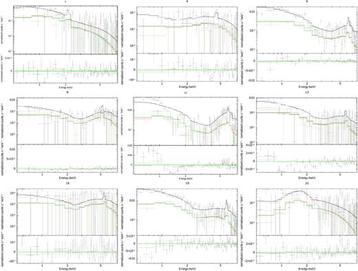
The XMM–Newton spectra of the nine sources that show indications of high amounts of obscuration in the X-rays (see the text). The best-fitting models are those described in Tables 5 and 6. In red and green colours, we plot the MOS-1 and MOS-2, and in black the pn counts. The residuals of each fit are also shown. (The colour figure is available in the online version.)
The X-ray spectral fits using two power-law components and an Fe Kα line.
| Number | z | NH | EW | C-stat |
|---|---|---|---|---|
| (1) | (2) | (3) | (4) | (5) |
| 1 | 1.973 | <56 | |$0.74^{+0.66}_{-0.44}$| | 2071/2498 |
| 4 | 0.526 | |$120^{+66}_{-44}$| | |$0.20^{+0.33}_{-0.20}$| | 2729/2498 |
| 6 | 0.039 | |$87^{+39}_{-27}$| | |$0.19^{+0.14}_{-0.13}$| | 2219/2498 |
| 9 | 0.210 | |$81^{+27}_{-22}$| | |$0.50^{+0.30}_{-0.22}$| | 1476/2498 |
| 12 | 0.027 | |$71^{+13}_{-11}$| | <0.20 | 1851/2498 |
| 13 | 0.094 | |$40^{+51}_{-19}$| | |$0.41^{+0.6}_{-0.27}$| | 2239/2498 |
| 18 | 0.184 | |$45^{+300}_{-38}$| | <0.60 | 2722/2498 |
| 19 | 0.077 | |$29^{+12}_{-9}$| | |$0.48^{+0.21}_{-0.16}$| | 2613/2498 |
| 20 | 2.560 | |$31^{+11}_{-8.5}$| | <0.20 | 1440/2498 |
The columns are: (1) source number; (2) redshift; (3) intrinsic hydrogen column density in units of 1022 cm−2; (3) equivalent width of the Fe Kα line in units of keV; (4) C-statistic/degrees of freedom. Both power-law spectral slopes are fixed to Γ = 1.8.
The X-ray spectral fits using a reflection model.
| Number | z | EW | C-stat |
|---|---|---|---|
| (1) | (2) | (3) | (4) |
| 4 | 0.53 | <0.41 | 2727/2500 |
| 18 | 0.184 | <0.85 | 2727/2500 |
| Number | z | EW | C-stat |
|---|---|---|---|
| (1) | (2) | (3) | (4) |
| 4 | 0.53 | <0.41 | 2727/2500 |
| 18 | 0.184 | <0.85 | 2727/2500 |
The columns are: (1) source number; (2) redshift; (3) equivalent width of the Fe Kα line in units of keV; (4) C-statistic/degrees of freedom.
The five sources which present a flat spectral index (# 4,6,12,18,19) are similar to the flat-spectrum CT candidates of Georgantopoulos et al. (2013) in the Chandra Deep Field South (CDFS) and Lanzuisi et al. (2013) in the Cosmological Evolution Survey field. A flat spectrum alone cannot constitute a CT source; more evidence is needed in the form of a high-EW Fe Kα line (EW ≳ 500 eV; see George & Fabian 1991). According to Table 5, only one of the flat sources (# 19) has a relatively strong line, with |${\rm EW}=480^{+210}_{-160}\,\mathrm{eV}$|, making it the second possible CT AGN of our sample, based on the X-ray spectra. Moreover, for the five flat sources, we use an alternative fit with a reflection component model (Magdziarz & Zdziarski 1995) plus a Gaussian line (wa*(pexrav+zga) in xspec notation). We fix the incident power-law component to Γ = 1.8 and the cosine of the inclination angle of the reflecting slab to 0.45. Again the energy of the Fe Kα line has been fixed to a rest-frame energy of 6.4 keV. For three of the five sources, the reflection model is excluded at over the 99.9 confidence level; the results of the fits for the rest are given in Table 6, where no significant detection is made of an Fe Kα line.
Optical spectra
In this section, we try to investigate the effectiveness of the selection methods used by invoking another parameter frequently used to select heavily obscured AGNs, the hard X-ray-to-[O iii] 5007 line flux ratio. In Fig. 7, we plot it against the hydrogen column density as calculated using the X-ray spectral fits in Tables 4 and 5. The [O iii] 5007 line is thought to arise from the narrow-line region and its flux is well correlated with the hard X-ray (2–10 keV) flux for both Seyfert-1 and Seyfert-2 sources, independent from the inclination angle (e.g. Alonso-Herrero, Ward & Kotilainen 1997). It is therefore considered an isotropic indicator of the intrinsic AGN flux. The hard X-ray-to-[O iii] 5007 line flux ratio has been used as a diagnostic for X-ray absorption in a number of studies (e.g. Maiolino et al. 1998; Bassani et al. 1999; Cappi et al. 2006; Vignali, Alexander & Comastri 2006; Akylas & Georgantopoulos 2009; Goulding et al. 2011). In Fig. 7, we use the updated X-ray fluxes from the spectral fits where available and keep the same colour coding as in Fig. 5, plotting sources which are no longer X-ray underluminous with respect to the mid-infrared with open symbols. The [O iii] fluxes are taken from the SDSS data base and are corrected for extinction using the relative intensity of the Balmer lines (|$f_{\rm [O\,\small {III}],cor}=f_{\rm [O\,\small {III}],obs}[{\rm (H\alpha /H\beta )/(H\alpha /H\beta )_{0}}]^{2.94}$|) and assuming and intrinsic Balmer decrement of (Hα/Hβ)0 = 2.76 (see Brocklehurst 1971). The solid line represents the expected correlation of the two quantities assuming an X-ray spectrum in the form of an absorbed power law with Γ = 1.8 and a reflection/scattered component of 1 per cent of the intrinsic flux. The normalization is taken from Akylas & Georgantopoulos (2009) and the dotted lines represent the 3σ limits of the correlation of the Seyfert-1 sample of Akylas & Georgantopoulos (2009). Note that the limits used by Maiolino et al. (1998) and Cappi et al. (2006) are within those boundaries.
![Hydrogen column density versus $f_{\rm x}/f_{\rm [O\,\small {III}]}$ ratio for all heavily obscured AGN candidates with [O iii] flux measurements in the SDSS. The X-ray fluxes come from the spectral fits whenever possible, otherwise measured in Georgakakis & Nandra (2011) and the [O iii] fluxes are corrected for extinction using the Balmer decrement. The NH values are the ones using a single power law (Table 4), except for sources also listed in Table 5, where two power-law components are fitted. The colour coding used is the same as in Fig. 5, with the open symbols representing non-X-ray underluminous sources. The red cross marks a possibly CT source (# 19). The curves are taken from Akylas & Georgantopoulos (2009) and represent the correlation expected for a power-law X-ray spectrum with Γ = 1.8 and a 1 per cent reflection/scattered component, normalized at NH = 0 at the mean for Seyfert-1 sources, ±3σ. The orange symbols show the difference in measured NH values for two nearby CT sources, when observed with Einstein (low-quality data, low energies, low NH) and BeppoSAX (higher quality data, higher energies, higher NH). (The colour figure is available in the online version.)](https://oup.silverchair-cdn.com/oup/backfile/Content_public/Journal/mnras/438/1/10.1093_mnras_stt2228/1/m_stt2228fig7.jpeg?Expires=1716421138&Signature=xs-VspcWn8ctedlGrkDpZhukvKizB3uVvdOAErvHGUjClt8BdUPrhQGHTl-5Yw7Rb36llHB~FKmdD7DCxM46~thBaoDqgx42-IVAw2HbPqp9hR87dKxLt8Erj5VaPqL53Apt81knc88uGILbYKZ6blYvVFOOZ~UViIiuIoTAXtbCxdlCbH8s14eIbMEBh5Jzrbk~IhvEcukdqIN4ayZr3L9agkE2PtiU6uU-QSXz2qA32PX7-iGZvuy9BTAbuskX6HCFyKPntwwdIbZKCyC5Z4x8pxuG0C48LZbVsn~w7p1FqpXEhzd~OiRfsFMtifRp7WAfKRWpNo8z9Eh6lpaGaA__&Key-Pair-Id=APKAIE5G5CRDK6RD3PGA)
Hydrogen column density versus |$f_{\rm x}/f_{\rm [O\,\small {III}]}$| ratio for all heavily obscured AGN candidates with [O iii] flux measurements in the SDSS. The X-ray fluxes come from the spectral fits whenever possible, otherwise measured in Georgakakis & Nandra (2011) and the [O iii] fluxes are corrected for extinction using the Balmer decrement. The NH values are the ones using a single power law (Table 4), except for sources also listed in Table 5, where two power-law components are fitted. The colour coding used is the same as in Fig. 5, with the open symbols representing non-X-ray underluminous sources. The red cross marks a possibly CT source (# 19). The curves are taken from Akylas & Georgantopoulos (2009) and represent the correlation expected for a power-law X-ray spectrum with Γ = 1.8 and a 1 per cent reflection/scattered component, normalized at NH = 0 at the mean for Seyfert-1 sources, ±3σ. The orange symbols show the difference in measured NH values for two nearby CT sources, when observed with Einstein (low-quality data, low energies, low NH) and BeppoSAX (higher quality data, higher energies, higher NH). (The colour figure is available in the online version.)
In Fig. 7, we keep the colour notation of Fig. 5 and plot the more robustly detected AGN SEDs in red colour. We can see that all the candidate sources for which we have a measurement of the [O iii] flux in the SDSS lie on the left of the mean |$f_{\rm x}/f_{\rm [O\,\small {III}]}$| found in Akylas & Georgantopoulos (2009), implying some degree of obscuration. It is interesting that source # 10 for which there is no solid evidence in the X-rays for the presence of a heavily obscured or CT nucleus is leftwards of the dotted line. For this source, the presence of a heavily obscured nucleus is implied by both a low X-ray-to-mid-infrared luminosity ratio and a low X-ray-to-[O iii] flux ratio, but it cannot be seen in the broad-band X-ray spectrum. One possibility is that the X-ray flux is variable, as the X-ray, optical and infrared observations are not taken at the same epoch. Another possibility is that we do not find any evidence in the X-rays because of the poor quality of the X-ray spectra, especially in the hard band. In Fig. 7, we plot as orange symbols the values for two well-known nearby CT AGNs, NGC 1068 and Mrk 3. The low-NH stars are measurements of the hydrogen column density based on early spectra taken with the Einstein Observatory (Kruper, Canizares & Urry 1990) and the high-NH stars are based on spectra taken with BeppoSAX, which extend to very high energies (Cappi et al. 1999; Guainazzi et al. 1999). The |$f_{\rm x}/f_{\rm [O\,\small {III}]}$| values are taken from Bassani et al. (1999). Both sources have a prominent soft excess attributed to a scattered component, which could be mistaken overall for a steep power law if the high-energy measurements were missing, or if the quality was poor. We therefore assume that part, or all, of the sources plotted in Figs 5 and 7 could be heavily obscured despite the fact that there is no apparent evidence in their XMM–Newton spectra.
Normal galaxies
Galaxies that do not host an AGN can also produce X-rays because of their star formation activity (see e.g. Ranalli et al. 2003, 2012; Rovilos et al. 2009). According to the hard X-ray-to-infrared relation of Ranalli et al. (2003): |$\log (L_{\rm 2{\rm -}10\,keV})=\log (L_{\rm FIR})-(3.62\pm 0.29)$|. If we use the 105 SED templates of Chary & Elbaz (2001) to calculate the ratio between the integrated FIR luminosity and the monochromatic luminosity at 12 μm, we find log (LFIR) = log (νLν(12 μm)) + (0.9 ± 0.2) for the star formation component. The integrated-to-monochromatic luminosity relations are best described by a broken power law (see Chary & Elbaz 2001); however, for the purpose of this study we keep the simplistic approach of a linear relation. From these relations, we expect that for a normal galaxy, the X-ray-to-mid-infrared ratio will be |$\log (L_{\rm 2{\rm -}10\,keV}/\nu L_{\nu }(\rm 12\,\mu \mathrm{m}))=-2.72\pm 0.35$|. Moreover, normal galaxies generally have soft X-ray spectra (see e.g. Ranalli et al. 2003; Lehmer et al. 2008). The mid-infrared luminosity we measure here comes from the torus component, after having performed a decomposition of the SED. In previous works looking for low X-ray–IR AGNs (e.g. Georgakakis et al. 2010), the contamination from normal galaxies is coming predominantly from sources that show no evidence for an AGN in their mid-infrared spectra (see also Pope et al. 2008). Therefore, we are not expecting a significant number of normal galaxies in the low X-ray-to-mid-infrared luminosity sample. Indeed, there are only three sources with |$L_{\rm 2{\rm -}10\,keV}/\nu L_{\nu }(\rm 12\,\mu \mathrm{m})<2.37$| and HR < −0.35, and for one of them the torus component is not statistically significant, which demonstrates the significance of the SED decomposition performed.
DISCUSSION
In this paper, we select a number of heavily obscured AGN candidates based on the ratio between their X-ray and mid-infrared luminosities. The AGNs produce high-energy emission close to the black hole, which heats the dust surrounding the nucleus and is re-emitted in the infrared. Thermal equilibrium of the hot dust in combination with the clumpiness of the medium (see Gandhi et al. 2009; Hönig & Kishimoto 2010; Hönig et al. 2010) causes the infrared emission to peak in relatively short wavelengths ( ∼ 10 μm). We use this property of the AGN infrared emission to separate it from the infrared emission from circumnuclear, or host galaxy star formation, whose SED peaks at ∼ 100 μm. Our selection of highly obscured AGN candidates is based on the assumed suppression of the X-ray luminosity with respect to the infrared.
There are 20 heavily obscured AGN candidates, and we look into their X-ray, optical and infrared properties in greater detail. A more detailed SED decomposition using optical-to-far-infrared photometry and a three-component fit finds a statistically significant contribution from a warm dust (torus) component in all 20 candidates; however, half of them are still X-ray underluminous if we take into account their infrared flux lower limits. We call those sources the ‘robust’ sample. Looking into the X-ray properties of all 20 candidates, we find evidence of high X-ray obscuration in nine sources (see Table 4; Fig. 6), and we call this the ‘X-ray obscured’ sample. We also investigate the [O iii] line luminosities in the SDSS optical spectra, and comparing them with the observed X-ray luminosities we find evidence for obscuration for seven sources with optical spectra.
Comparison with other selection methods
In this section, we compare the results of our method with others used in the literature.
25 μm selection
Recently, Severgnini et al. (2012) used a similar technique with the one used here to detect nearby CT sources, comparing the 2–12 keV X-ray flux and the total 25 μm infrared flux, and using the hardness ratio between the 2–4.5 and 4.5-12 keV bands of XMM–Newton (HR4), they found that ∼84 per cent of AGNs with |$f_{\rm 2{\rm -}12\,keV}/\nu f_{\nu }{\rm (25\,\mu \mathrm{m})}<0.02$| and HR4 > −0.2 show CT characteristics in their X-ray spectra (see fig. 1 of Severgnini et al. 2012). In Fig. 8, we plot the equivalent plot for the XMM–WISE sample, using the |$L_{\rm 2{\rm -}10\,keV}/\nu L_{\nu }{\rm (12\,\mu \mathrm{m})}$| and HR thresholds described in Section 4.2 and the |$L_{\rm 2{\rm -}10\,keV}$| values derived from the spectral fits. We plot the sources with robustly detected (>2σ) infrared AGN components with black circles, and the rest in grey. We use luminosities instead of fluxes here in order to take into account the different k-corrections for each source, since our sample expands to relatively high redshifts; the sample of Severgnini et al. (2012) on the other hand consists of local sources, where the k-correction is negligible. The vertical line is at HR = −0.35, and the grey area represents the range of |$L_{\rm 2{\rm -}10\,keV}/\nu L_{\nu }{\rm (12\,\mu \mathrm{m})}$| threshold values within the range of |$L_{\rm 2{\rm -}10\,keV}=10^{41.5}{\rm -}10^{45}\,{\rm erg\,s^{-1}}$|, since the relation of Gandhi et al. (2009) is not linear, and a simple |$L_{\rm 2{\rm -}10\,keV}/\nu L_{\nu }{\rm (12\,\mu \mathrm{m})}$| threshold cannot characterize our selection. We use the same symbols as in Fig. 7 for the 20 sources of our sample.
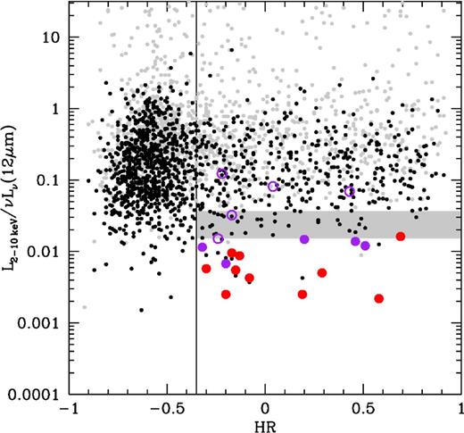
The X-ray-to-mid-infrared luminosity ratio plotted against the X-ray hardness ratio for all the X-ray–mid-infrared sample. We plot the sources with robustly detected (>2σ) infrared AGN components with black circles, and the rest in grey. The vertical line marks the HR = −0.35, which we use to differentiate between soft and hard X-ray sources. The grey area marks the |$L_{\rm 2{\rm -}10\,keV}/\nu L_{\nu }(\rm 12\,\mu \mathrm{m})$| threshold marked with the solid line in Fig. 4 with the limiting luminosities set to |$L_{\rm 2{\rm -}10\,keV}^{\rm min}=10^{41.5}\,{\rm erg\,s^{-1}}$| and |$L_{\rm 2{\rm -}10\,keV}^{\rm max}=10^{45.0}\,{\rm erg\,s^{-1}}$|. We keep the same symbols for the sources in our sample as in Fig. 7. (The colour figure is available in the online version.)
Using the SED decomposition technique described earlier we also have a measure of the AGN monochromatic luminosity in the 25 μm band. If we apply an |$L_{\rm 2{\rm -}10\,keV}/\nu L_{\nu }{\rm (25\,\mu \mathrm{m})}$| limit of 0.02, as in Severgnini et al. (2012), and our HR limit of –0.35, we find the same 17 of the 20 sources of our sample (and all the ‘robust’ ones), plus four sources that could be CT candidates and are not in the low |$L_{\rm 2{\rm -}10\,keV}/\nu L_{\nu }{\rm (12\,\mu \mathrm{m})}$| sample. However, the 25 μm luminosity measurement is an extrapolation from the best-fitting SED, except for sources with a 22 μm flux measurement at z > 1.14. For the four sources, the |$L_{\rm 2{\rm -}10\,keV}/\nu L_{\nu }{\rm (12\,\mu \mathrm{m})}$| values are very close to the limit used in this paper, so they are considered statistical fluctuations. Therefore, we conclude that selecting CT candidates using the 25 μm instead of the 12 μm luminosity would not yield a significantly different sample, and therefore our selection is very similar to the one used by Severgnini et al. (2012).
WISE colour–colour selection
The WISE catalogue provides photometry in four different mid-infrared bands, so different colour–colour techniques have been proposed to select AGNs, similar to the techniques used for Spitzer–Infrared Array Camera (IRAC) sources (e.g. Lacy et al. 2004; Stern et al. 2005; Donley et al. 2012). A useful selection is the three-band colour–colour diagram using the 3.4, 4.6 and 12 μm bands, where optically and radio-selected quasi stellar objects (QSOs) occupy a distinct region (e.g. Yan et al. 2013). Seyfert galaxies (spectroscopically identified) in Yan et al. (2013) however lie in a similar region to that occupied by starbursts. Similarly, Mateos et al. (2012) defined a region in the [3.4] − [4.6] versus [4.6] − [12] diagram where the bulk of the X-ray luminous (|$L_{\rm 2{\rm -}10\,keV}>10^{44}\,{\rm erg\,s^{-1}}$|) AGNs are located, which lies around the line defined by a power law (fν ∝ να) with α < −0.3 (see also Alonso-Herrero et al. 2006; Donley et al. 2007). Stern et al. (2012) argue that a similar result is reached when the selection is made using only the [3.4] − [4.6] colour, with [3.4] − [4.6] > 0.8, and find that the technique has similar properties to the Spitzer–IRAC selection of Stern et al. (2005). However, there is a dependence of both the reliability and the efficiency of the method on the flux limits used, as previously claimed (e.g. Barmby et al. 2006; Brusa et al. 2009; Rovilos et al. 2011; Mendez et al. 2013).
In Fig. 9, we plot the [3.4] − [4.6] versus the [4.6] − [12] colours for all the sources in our sample. The black contours represent the density in the [3.4] − [4.6]–[4.6] − [12] parameter space of all of the WISE sources that lie within a 1 arcmin radius of an X-ray source, therefore an infrared-selected sample, or a ‘background’ sample, since the vast majority of the infrared sources out to this radius are chance matches to the X-ray sources. The contours represent regions with point densities of 100–1000 sources per 0.2 × 0.2 mag2 pixel, with a step of 100. The region where the 2844 X-ray sources with fitted infrared SEDs lie is represented with the blue contours, with 15–90 sources per 0.2 × 0.2 mag2 pixel, with a step of 15. This is the region where the moderate X-ray luminosity AGNs lie (2181/2844 have |$L_{\rm 2{\rm -}10\,keV}<10^{44}\,{\rm erg\,s^{-1}}$|) and it is different from the background, although the highest density point is not in the ‘QSO region’ of Mateos et al. (2012), marked with the solid lines, or above the ‘QSO limit’ of Stern et al. (2012), marked with the dashed line. These selection criteria are reliable for selecting the 661 sources with |$L_{\rm 2{\rm -}10\,keV}\ge 10^{44}\,{\rm erg\,s^{-1}}$|, plotted with green circles. This is indicative of the contamination of the mid-infrared colours of AGNs by the host galaxy; Del Moro et al. (2013) find that the fraction of AGNs detected in the mid-infrared using SED decomposition increases with increasing X-ray luminosity. The WISE colours of the blue contour and the green circles regions are in good agreement with the WISE colours of the [O iii]-selected and hard-X-ray-selected AGNs, respectively, of Mateos et al. (2013), which again reflects on the X-ray luminosity distributions of those samples.
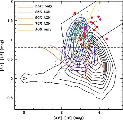
The WISE colour–colour diagram. The black contours represent all the infrared sources, while the blue contours represent the X-ray sources. The bulk of the X-ray sources is offset from the bulk of the infrared sources, but not in the area where most of the luminous X-ray sources reside, according to Mateos et al. (2012) (solid lines) and Stern et al. (2012) (dashed line). The AGNs with |$L_{\rm 2{\rm -}10\,keV}>10^{44}\,{\rm erg\,s^{-1}}$| are plotted with green dots, and the majority of them are in the aforementioned areas. The heavily obscured candidates are plotted in red and purple symbols, following Figs 7 and 8. Red crosses mark sources that have an indication of heavy obscuration in their X-ray spectra. The orange to yellow contours are the tracks of a pure host SED gradually contaminated with an AGN (torus) SED. (The colour figure is available in the online version.)
The red and purple points in Fig. 9 mark the colours of the 20 highly obscured AGN candidates, the red points representing the most robust sample and the open purple circles representing the sources which do not meet the initial Lx/Lir criteria if the X-ray luminosities are measured from the spectra. 8/10 and 10/10 of the red points, and 18/20 and 20/20 of all points comply with the criteria defined by Mateos et al. (2012) and Stern et al. (2012), respectively. It is interesting that for the points in Fig. 9 the fraction that comply with the ‘QSO selection’ criteria and have |$L_{\rm 2{\rm -}10\,keV}>10^{44}\,{\rm erg\,s^{-1}}$| is significantly smaller than that of the general AGN population: 4/18 (22.2 per cent) and 5/20 (20.0 per cent) of the red sources that comply with the Mateos et al. (2012) and Stern et al. (2012) criteria, respectively, have high X-ray luminosities, compared to 594/1483 (40.0 per cent) and 577/1258 (45.9 per cent), respectively, for the general X-ray source population. We keep the original X-ray luminosities for this discussion, because an a priori knowledge of the X-ray spectra is not possible. We attribute the difference to the obscuration of the X-rays. If we use the intrinsic X-ray luminosities calculated from the Gandhi et al. (2009) relation (column 5 of Table 2), the fractions become 12/18 (66.7 per cent) and 13/20 (65.0 per cent), even higher than that of the overall X-ray population, showing that the ‘infrared-selected’ sample is not clean (see also Georgantopoulos et al. 2011). Georgantopoulos et al. (2011) find that the X-ray-to-mid-infrared luminosity selection appears to be complete in the local universe and incomplete at higher redshifts; here we find signs of incompleteness in the local universe (all four sources have z < 0.04), which is potentially even higher, since all our candidates were initially selected using a mid-infrared criterion.
The mid-infrared colours can be used as an indication of the contamination of the mid-infrared flux by the host galaxy (see Rovilos et al. 2011). This is also evident if we plot in Fig. 9 the track of a pure starburst galaxy from the Chary & Elbaz (2001) library used for the SED decomposition, and gradually add a torus template from the Silva et al. (2004) sample; this is seen going from orange to yellow tracks in Fig. 9. The 25 per cent step refers to the fraction of 12 μm monochromatic flux coming from the torus template, and the redshift range is 0 ≤ z ≤ 2, with a circle marking z = 0 and z = 1. In this case, the high percentage of X-ray luminous sources in the ‘QSO selection’ regions shows that the highest X-ray luminosity AGNs are less contaminated by the host galaxy in the mid-infrared wavelengths (see also Del Moro et al. 2013). This trend is not as strong for the CT candidates, which is a direct implication of their selection criterion (low Lx/Lir), meaning that the obscuration is affecting the X-rays more than the infrared wavelengths. It is also interesting that 6/20 and 5/20 of the infrared-selected candidates would not have been selected if we used a selection scheme based on a combination of the Mateos et al. (2012) or Stern et al. (2012) criterion, respectively, and a low observed X-ray luminosity threshold (e.g. |$L_{\rm 2{\rm -}10\, keV}<10^{44}\,{\rm erg\,s^{-1}}$|). The reason for this is that the SED decomposition is more accurate in identifying the AGN component from the mid-infrared photometry than a simple colour–colour selection, as it uses more information (more infrared bands), and the statistics are easier to handle and interpret.
Number of heavily obscured AGNs
We use three indicators for a heavily obscured AGN, the X-ray spectrum, the X-ray-to-mid-infrared luminosity ratio and the X-ray-to-[O iii] line flux ratio. For the latter, we assume a ratio of |$f_{\rm 2{\rm -}10\,keV}/f_{\rm [O\,\small {III}]}=1.0$|, on the dotted line of Fig. 7 for low column densities. In Table 7, we present the results of the three indicators: we use a ‘✓’ symbol for a positive indication, a ‘×’ symbol for negative and a ‘–’ symbol for no indication, or an inconclusive indication. For 9 of the 20 candidates # 2,6,9,10,11,12,13,19,20 there are two or more indicators for the presence of a heavily obscured AGN, and another three (# 1,4,18) are heavily obscured according to their X-ray spectra, which is the most reliable indicator. Four sources (# 3,8,14,16) are heavily obscured candidates from their mid-infrared luminosities with no information from either their X-ray spectra or the [O iii] flux, and three (# 7,15,17) have low X-ray-to-mid-infrared luminosities, while their X-ray spectra argue against them being heavily obscured; they could be either variable sources, or their obscuration might be missed in the X-rays because of their low X-ray fluxes. Those three sources (along with source # 10 which has no obscuration indication in the X-rays but is heavily obscured according to both its infrared and its [O iii] luminosity) are the faintest sources with fitted spectra in our candidate sample and their spectra are expected to be of low quality, so that an obscured nucleus can easily be missed. Finally, source # 5 has no indications of obscuration. The CT sources are even fewer: we have direct indications from the X-ray spectra for two sources (# 4,19), and another two (# 2,11) are X-ray underluminous with respect to both the mid-infrared and the [O iii] luminosities, while they are too faint in the X-rays for a useful spectrum to be extracted. Finally, source # 10 is in the robust mid-infrared sample, with its X-ray-to-[O iii] flux ratio indicating that it is CT; there is no indication in its X-ray spectrum, but it has the lowest number of counts of all the sources with fitted spectra. Summing up, there are 12–19 heavily obscured AGNs in the sample, and 2–5 of them are CT.
Obscuration tests: ‘✓’ indicates an obscured AGN, ‘×’ an unobscured AGN and ‘–’ inconclusive or no indication.
| Number | Mid-IR | X-rays | [O iii] |
|---|---|---|---|
| (1) | (2) | (3) | (4) |
| 1 | × | ✓ | – |
| 2 | ✓✓ | – | ✓ |
| 3 | ✓ | – | – |
| 4 | × | ✓ | – |
| 5 | × | × | × |
| 6 | ✓✓ | ✓ | ✓ |
| 7 | ✓ | × | – |
| 8 | ✓✓ | – | – |
| 9 | ✓✓ | ✓ | ✓ |
| 10 | ✓✓ | × | ✓ |
| 11 | ✓✓ | – | ✓ |
| 12 | × | ✓ | ✓ |
| 13 | ✓ | ✓ | ✓ |
| 14 | ✓ | – | – |
| 15 | ✓ | × | – |
| 16 | ✓✓ | – | – |
| 17 | ✓✓ | × | – |
| 18 | × | ✓ | – |
| 19 | ✓✓ | ✓ | × |
| 20 | ✓✓ | ✓ | – |
| Total | 15(10)/20 | 9/14 | 7/9 |
The columns are: (1) source number; (2) |$L_{\rm 2{\rm -}10\,keV}/\nu L_{\nu }{\rm (12\,\mu \mathrm{m})}$| being significantly lower than the Gandhi et al. (2009) relation. A double ‘✓’ mark notes that the 2σ lower limit in νLν(12 μm) is still below the relation; (3) detection of an Fe Kα line or a flat X-ray spectrum; (4) |$f_{\rm 2{\rm -}10\,keV}/f_{\rm [O\,\small {III}]}<1.0$|.
We compare the above numbers to the predictions of X-ray background synthesis models for the number of heavily obscured (NH ∼ 1023-1024 cm− 2) and CT AGNs expected in the current XMM/WISE survey. X-ray background synthesis models predict the number of CT AGNs using as constraints the spectrum of the X-ray background and/or the number of CT AGNs observed in very hard (>10 keV) X-ray surveys performed with Swift and INTEGRAL at bright fluxes. There have been several X-ray background synthesis models publicly available online (e.g. Gilli, Comastri & Hasinger 2007; Draper & Ballantyne 2009; Treister, Urry & Virani 2009; Akylas et al. 2012). We choose to work with the model of Akylas et al. (2012), as this model uses the most updated constraints on the number of CT AGNs observed in the local Universe with Swift (Burlon et al. 2011). We use the area curve of our XMM–Newton survey as given in Georgakakis & Nandra (2011) and assume an intrinsic CT fraction of 15 per cent, which is the best-fitting model in Akylas et al. (2012). We find a fraction of heavily obscured and CT AGNs of 12 and 0.8 per cent, respectively. Given that we fit the SEDs of 2844 sources in our sample (those with a hard band detection, either spectroscopic or photometric redshift, and three or more infrared photometry data points), we expect 23 and 342 CT and heavily obscured AGNs, respectively. These numbers are well above the numbers found in the previous paragraph (2–5 and 12–19). This discrepancy can be explained if there are highly obscured sources that do not present a low X-ray-to-mid-infrared luminosity ratio, and therefore they are not selected by our selection procedure. This is the case for two CT AGNs in the XMM–CDFS observations of Comastri et al. (2011). Georgantopoulos et al. (2011) discuss that these have a high X-ray-to-mid-infrared luminosity ratio typical of unobscured AGNs. Moreover, we have included here an initial selection of sources that have a redshift determination in the SDSS, which means that we are not including a large number of optically faint sources, which are on average more obscured in the X-rays than the general X-ray population (see e.g. Civano, Comastri & Brusa 2005; Rovilos et al. 2010).
Another factor which we have to include when assessing the number of heavily obscured AGNs found with the low X-ray-to-mid-infrared luminosity method is the scatter in the X-ray-to-mid-infrared flux relation. Detailed analysis of the nuclear regions of local Seyferts done by Gandhi et al. (2009) finds a relation with a scatter of 0.23 dex for the well-resolved sample and 0.36 dex for the full sample. Including more sources and low-luminosity AGNs, Asmus et al. (2011) find a similar relation with a similar scatter (0.35 dex). Georgakakis et al. (2010) find that the host contribution to the infrared flux can affect the X-ray-to-infrared ratio, and in this work we remove the host contribution from the infrared flux using SED decomposition. We find a scatter in the Lx-LMIR relation of 0.5 dex, larger than that found by both Gandhi et al. (2009) and Asmus et al. (2011). Part of our scatter can be introduced by X-ray absorption, which is not corrected for, and another part is a result of the Γ = 1.4 assumption made in calculating the X-ray luminosities. Comparing the X-ray luminosities in Tables 2 and 4, we can see that in some cases they can differ up to one order of magnitude. Removing this source of scatter would require fitting the X-ray spectra of all the 2844 sources, which is not feasible. We have removed it for 14 sources of our sample and indeed 5 of them are no longer low X-ray-to-mid-infrared candidates, but we do not have information on how many sources would make it into the mid-infrared-selected sample if we corrected all the sources.
In summary, the X-ray-to-mid-infrared luminosity ratio technique is somewhat reliable for finding obscured sources, i.e. most low X-ray-to-IR luminosity sources have large amounts of obscuration. However, the technique suffers from incompleteness, because of the selection made in optical–infrared wavelengths and because of the scatter of the Lx-LMIR relation, introduced by observational constraints.
CONCLUSIONS
In this work, we combine the XMM–SDSS survey with the all-sky mid-infrared survey of WISE to select highly obscured AGNs. We use only sources detected in the hard X-ray band (2–8 keV) in order to have an initial estimate of the hardness ratio and therefore avoid normal galaxies, whose X-ray emission does not originate from an AGN and have similar X-ray-to-infrared luminosity ratios to heavily obscured AGNs, and other unobscured sources. We also use only X-ray sources that have an SDSS counterpart bright enough to provide a spectroscopic or photometric redshift, and with a detection in at least three bands with WISE and 2MASS to be able to perform SED fitting. These selections limit the initial number of sources from 39 830 to 2844. Out of those sources, we select 20 heavily obscured AGN candidates on the basis of their low X-ray-to-mid-infrared luminosity ratios and relatively hard X-ray spectra (HR > −0.35; Γ < 1.4). We then investigate further their optical-to-far-infrared SEDs using a three-component fit, their optical properties (spectra) and their X-ray spectra from XMM–Newton. Our results are summarized as follows.
Detailed SED decomposition using photometry from the near-ultraviolet to the far-infrared and three components (stellar, AGN, star formation) finds robust evidence for the presence of a luminous AGN component in the infrared for all 20 sources.
The broad-band X-ray spectra indicate the presence of a heavily obscured AGN in 9 out of the 14 sources for which X-ray spectra could be fitted. The X-ray criteria used are either: (i) the presence of a high-EW Fe Kα line, (ii) a flat spectral index, (iii) a reflection component, or a combination of the three.
We have an [O iii] 5007 line measurement for 9 out of 20 heavily obscured candidates, and assuming a threshold of |$f_{\rm 2{\rm -}10\,keV}/f_{\rm [O\,\small {III}]}=1.0$|, 7 of them are likely to host an obscured AGN.
Taking all the above criteria into account, we deduce that the number of heavily obscured sources selected with our method is 12–19, with 2–5 of them being CT. This number is a factor of 20 less than what would be expected from X-ray background population synthesis models for heavily obscured AGNs, and a factor of 5 for CT AGNs. We attribute those differences to the initial selection method based on a relatively high mid-infrared luminosity and an optical detection, characteristics not shared by many obscured AGNs, and the scatter of the Lx-LMIR relation. This shows the limitations of this method for selecting large numbers of heavily obscured AGNs in wide shallow surveys.
We test popular obscured AGN selection methods based on mid-infrared colours, and find that the probability of an AGN to be selected by its mid-infrared colours increases with the intrinsic X-ray luminosity, while the (observed) X-ray luminosities of heavily obscured AGNs are relatively low (|$L_{\rm 2{\rm -}10\,keV}<10^{44}\,{\rm erg\,s^{-1}}$|). In fact, a selection scheme based on a relatively low X-ray luminosity and QSO mid-infrared colours would not select a quarter of the heavily obscured AGNs of our sample.
The research leading to these results has received funding from the People Programme (Marie Curie Actions) of the European Union's Seventh Framework Programme (FP7/2007–2013) under REA grant agreement number 298480. DMA, ADM and JRM thank the Science and Technology Facilities Council (STFC) and the Leverhulme Trust for support. AC acknowledges financial contribution from the agreement ASI–INAF I/009/10/0 and INAF–PRIN 2011. PG acknowledges support from STFC grant reference ST/J00369711. This publication makes use of data products from the Wide-field Infrared Survey Explorer, which is a joint project of the University of California, Los Angeles, and the Jet Propulsion Laboratory/California Institute of Technology, funded by the National Aeronautics and Space Administration.
The likelihood ratio method (Sutherland & Saunders 1992) is usually adopted in the cases where a counterpart is sought in a crowded catalogue (in this case the SDSS catalogue), and it uses the surface density of objects of a given magnitude to estimate the probability that a counterpart at a certain distance is a chance match.
REFERENCES
APPENDIX A: SED FITTING DETAILS
In the general case of three-component fitting (including synthetic stellar templates), we have three sets of templates, codenamed ‘stellar’, ‘SB’ and ‘AGN’. For the stellar templates, we use the Bruzual & Charlot (2003) stellar population models, with solar metallicity and a range of star formation histories and ages; in total we use 75 templates. We then redden each template using a Calzetti et al. (2000) dust extinction law, with a range of E(B − V) from 0 to 2 in steps of 0.1. This gives us a library of 1500 synthetic stellar templates. For the SB templates, we use the library of Chary & Elbaz (2001) (105 templates), or the library of Mullaney et al. (2011) (5 templates), which we crop at rest-frame wavelengths below 4.5 μm in order not to duplicate the stellar population, since it is the main contributor in the optical–near-infrared wavelengths in the Chary & Elbaz (2001) templates. For the AGN templates, we use the library of Silva et al. (2004), which includes five templates: four of them are ‘torus’ templates with varying extinction ranging from NH = 0 to NH = 1024 cm−2 and the fifth is the NH = 0 template with a blue bump.
We use a Monte Carlo Markov chain (MCMC) sampling method for the SED fitting, taking into consideration all the possible combinations of templates (1500 × 105 × 5 or 1500 × 5 × 5). For each combination, we calculate the minimum and maximum contribution of each component, we reduce the minimum contribution by a factor of 100 and use this range to vary the contribution of each template with the MCMC sampling. For each ‘test combination’, we calculate the likelihood using equation (A1). As the best fit we keep the combination and normalization that gives the maximum likelihood. We keep the likelihood values of all trial fits and we plot their natural logarithm (log-likelihood) against key values corresponding to the given combination and normalizations. Examples of such plots are given in Fig. 3 – left-hand panel.
The resulting SED fits for the 31 candidate heavily obscured AGNs are shown in Fig. A1.
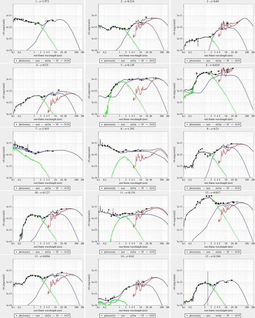
SED decomposition results using three templates (stellar, AGN, star formation), shown in the green, blue and red lines, respectively. The dark grey line shows the combination of the three templates and the black points and error bars denote the photometry data points, with the error bar on the x-axis representing the effective width of the filter. (The colour figure is available in the online version.)
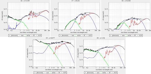
– continued
