


Abstract
Here we introduce crash3, the latest release of the 3D radiative transfer code crash. In its current implementation, crash3 integrates into the reference algorithm the code cloudy to evaluate the ionization states of metals, self-consistently with the radiative transfer through H and He. The feedback of the heavy elements on the calculation of the gas temperature is also taken into account, making crash3 the first 3D code for cosmological applications which treats self-consistently the radiative transfer through an inhomogeneous distribution of metal-enriched gas with an arbitrary number of point sources and/or a background radiation. The code has been tested in idealized configurations, as well as in a more realistic case of multiple sources embedded in a polluted cosmic web. Through these validation tests, the new method has been proven to be numerically stable and convergent. We have studied the dependence of the results on a number of physical quantities such as the source characteristics (spectral range and shape, intensity), the metal composition, the gas number density and metallicity.
INTRODUCTION
During the last decade, observational and theoretical studies constraining the nature of the intergalactic medium (IGM) have shown that metals are a pervasive component of the baryonic budget of our Universe and that they are associated with a wide range of hydrogen column density (|$N_{\mathrm{H {\small I}}}$|) systems typically identified in quasar (QSO) absorption spectra at different redshifts (Meyer & York 1987; Lu 1991; Songaila & Cowie 1996; Cowie & Songaila 1998; Ellison et al. 2000; Schaye et al. 2000, 2003; Songaila 2001; Aracil et al. 2004; Pieri & Haenhelt 2004; Becker et al. 2011; also see Meiksin 2009 for a review).
High H i column density absorbers, with |$N_{\mathrm{H {\small I}}}\geqslant 2\times 10^{20} \rm {cm}^{-2}$|, are easily identified in these spectra for the presence of strong damping wings, and are classified as damped Lyα systems (DLAs). Column densities in the range |$1.6\times 10^{17}\le N_{\mathrm{H {\small I}}}\le 10^{20} \rm {cm}^{-2}$| are instead associated with Lyman limit systems (LLSs) and spectroscopically identified by their strongly saturated Lyα lines. Both systems show C iv lines as well as many ions in lower ionization states (Mn ii, Si ii, Fe ii), and are typically associated with metallicities of Z ∼ 10−2 Z⊙ (LLSs; e.g. Steidel 1990) and 10−2 ≤ Z ≤ 0.3 Z⊙ (DLAs; e.g. Steidel 1990; Hellsten et al. 1997; Rauch, Haehnelt & Steinmetz 1997; Pettini et al. 1999; Kulkarni et al. 2005).
The presence of metals in LLSs and DLAs can be interpreted as a natural product of the stellar nucleosynthesis acting therein. LLSs are in fact identified as clouds in the galactic haloes, while high-redshift (z ∼ 3) DLAs are believed to be the progenitors of the present-day galaxies.
Advances in high-resolution spectroscopy revealed weak metal absorption lines in the Lyα forest (|$N_{\rm H {\small I}} \lesssim 10^{-17}$| cm−2), with C iv detected in most of the systems with |$N_{\mathrm{H {\small I}}}\geqslant 10^{15} \rm {cm}^{-2}$| and in more than half of the systems with |$N_{\mathrm{H {\small I}}}\geqslant 10^{14} \rm {cm}^{-2}$| (Tytler et al. 1995; Songaila & Cowie 1996). The typical metallicities of the Lyα forest are estimated in the range 10−4 ≤ Z ≤ 10−2 Z⊙ (Simcoe, Sargent & Rauch 2004). The subsequent discovery of a metallic component in less dense regions (Cowie & Songaila 1998; Ellison et al. 2000; Schaye et al. 2000, 2003; Aracil et al. 2004; Pieri & Haenhelt 2004) has been interpreted as the evidence of efficient spreading mechanisms which are able to transport the metals far away from their production sites and pollute low-density regions.
The redshift evolution of the gas metallicity has been extensively investigated. In the redshift range 1.5 < z < 4, C iv and Si iv doublets are the main tracers of the IGM metallicity, because their rest-frame wavelength is larger than the Lyα and the lines cannot be confused with those of the forest. In this range the column density distribution of C iv seems to remain constant (Songaila 2001). Although a consensus has not been reached yet, a decline in the abundance of C iv above z ∼ 4.5 is reported by different groups (Becker, Rauch & Sargent 2009; Ryan-Weber et al. 2009; Becker et al. 2011; Simcoe et al. 2011). The Si iv doublet λλ1393.76, 1402.77 Å has been investigated in QSO line surveys in the redshift range 1.5 < z < 5.5. Songaila (2001) measured |$\Omega _{\rm Si {\small IV}}$|, the Si iv mass density relative to the critical density, in the redshift range 2 < z < 5.5, finding a roughly constant value in the range 2 < z < 4.5 for absorbers with column densities |$10^{13} \le N_{\rm Si {\small IV}} \le 10^{15} {\rm cm}^{-2}$|, while |$\Omega _{\rm Si {\small IV}}$| may have increased by an order of magnitude in 4.5 < z < 5.5. These abundance trends have been confirmed by subsequent studies (Boksenberg, Sargent & Rauch 2003; Songaila 2005; Scannapieco et al. 2006).
At higher redshifts, a critical diagnostic role could be played instead by ions with lower ionization states like C ii, Si ii and O ii, probing colder gas (Oh 2002; Furlanetto & Loeb 2003; Becker et al. 2011).
Below z ∼ 1 a larger sample of data is available also for the oxygen component which is the major tracer of the IGM metallicity. The interested reader can find more information in the recent study of Cooksey et al. (2011), and references therein.
Beyond this general consensus, many observational data remain controversial, as well as their interpretation which is of primary importance, e.g. in constraining different enrichment scenarios. The metal abundance, the number of ionization states and the distribution in space and time are still subjects of intense debate (see Petitjean 2001, 2005).
The theoretical interpretation of the data is of particular relevance because observations of metals in dense regions, where stellar nucleosynthesis is active, provide a record of the star formation history, while observations in the IGM can be a good indicator of the galactic wind efficiency, the velocity structure of the IGM and more in general of the enrichment mechanism (Gnedin & Ostriker 1997; Ferrara, Pettini & Shchekinov 2000; Cen & Bryan 2001; Madau, Ferrara & Rees 2001). In fact, different scenarios have been considered in the literature, as an early enrichment by the first generation of stars (Madau et al. 2001), a continuous enrichment (Gnedin & Ostriker 1997; Ferrara et al. 2000; Scannapieco, Ferrara & Madau 2002), or a late enrichment coinciding with the star formation peak at z ∼ 2–4 (Adelberger et al. 2005). In addition, the determination of metal abundances could also constrain the efficiency of the gas cooling function (Sutherland & Dopita 1993; Maio et al. 2007; Smith, Sigurdsson & Abel 2008; Wiersma, Schaye & Smith 2009a) and the formation of massive galaxies (Thacker, Scannapieco & Davis 2002).
For these reasons, several theoretical schemes for metal production and spreading have been developed, based on both semi-analytic models (e.g. Scannapieco et al. 2002, 2006) and numerical simulations (Mosconi et al. 2001; Scannapieco et al. 2005; Oppenheimer & Davé 2006; Dubois & Teyssier 2007; Wiersma et al. 2009b; Maio et al. 2010; Schaye et al. 2010; Shen, Wadsley & Stinson 2010; Tornatore et al. 2010; Wiersma et al. 2010; Maio et al. 2011; Wiersma, Schaye & Theuns 2011). In the most advanced approaches, the ionization state of the metals is calculated assuming the presence of a uniform ultraviolet (UV) background, which is then used as energetic input for photoionization codes computing the metal ionization states at the equilibrium (Oppenheimer & Davé 2006; Oppenheimer, Davé & Finlator 2009; Oppenheimer et al. 2012). The results of this approach are affected by the uncertainties associated with the assumptions on the shape and intensity of the radiation field, which is not calculated self-consistently from the radiative transfer (RT) across the inhomogeneous gas distribution. Many studies suggest in fact that shadowing, filtering and self-shielding induce deviations in the shape and intensity of the background with respect to models in which the effects of the RT are neglected (Maselli & Ferrara 2005, and references therein).
Fluctuations in the photoionization rates as well as spatial deviations in the IGM temperature due to the inhomogeneity of the cosmic web support this view at least on scales of few comoving Mpc (see Maselli & Ferrara 2005; Furlanetto 2009; Meiksin 2009, and references therein). On larger scales (∼100 h−1 Mpc comoving) the source spatial distribution and their spectral variability could be an additional cause of variations in the UV background (Zuo 1992a,b; Meiksin & White 2003; Bolton & Viel 2011).
The fluctuations induced by RT effects could also be efficiently recorded in the ionization state of the metals, because their rich electronic structure and atomic spectrum are more sensitive, compared to H and He, to the radiation field fluctuations (Oh 2002; Furlanetto & Loeb 2003; Furlanetto 2009).
Numerical schemes that solve the cosmological RT equation by applying different approximations are now quite mature and well tested (Iliev et al. 2006a, 2009, and references therein, for an overview of the available codes) and are able to simulate complex scenarios involving large cosmological boxes and a number of sources (e.g. Ciardi, Stoehr & White 2003a; Ciardi, Ferrara & White 2003b; Iliev et al. 2006b; Trac & Cen 2007; McQuinn et al. 2009; Baek et al. 2010; Ciardi et al. 2012). Typically, these codes are restricted to the hydrogen chemistry, with only a few of them including a self-consistent treatment of the helium component, which is particularly relevant for a correct determination of the gas temperature (see e.g. Ciardi et al. 2012). None of them though includes the treatment of metal species.
In the interstellar medium (ISM) community, on the other hand, several photoionization codes, such as cloudy (Ferland et al. 1998), mappingsiii (Allen et al. 1998) and mocassin (Ercolano et al. 2003), are able to simulate the complex physics of galactic H ii regions largely polluted by heavy elements.
The aim of the present work is to describe a novel extension of the RT code crash (Ciardi et al. 2001; Maselli, Ferrara & Ciardi 2003; Maselli, Ciardi & Kanekar 2009a), which has been integrated with cloudy, allowing the prediction of metal ionization states self-consistently with the radiation field as calculated by the RT through the IGM density field.
The paper is structured as follows. In Sections 2 and 3, we briefly introduce the RT code crash and the photoionization code cloudy. In Section 4, we illustrate the details of the integration of the two codes into a self-consistent pipeline. The tests of the new crash variant called crash3 are reported in Section 5. Section 6 summarizes the conclusions.
CRASH
crash is a 3D RT code designed to follow the propagation of hydrogen ionizing photons (i.e. with energy E ≥ 13.6 eV) through a gas composed by H and He. The code adopts a combination of ray-tracing and Monte Carlo (MC) sampling techniques to propagate photon packets through an arbitrary gas distribution mapped on a Cartesian grid, and to follow in each grid cell the evolution of gas ionization and temperature. This treatment guarantees a reliable description of such evolution in a large variety of configurations, as shown by the Cosmological Radiative Transfer Comparison Project tests (Iliev et al. 2006a), and its various applications to the study of the H and He reionization (Ciardi et al. 2003a,b, 2012), the imprints of the fluctuating background on the Lyα forest (Maselli & Ferrara 2005), the quasar proximity effects (Maselli et al. 2007; Maselli, Ferrara & Gallerani 2009b) and the impact of reionization on the visibility of Lyα emitters (Dayal, Maselli & Ferrara 2011; Jeeson-Daniel et al. 2012).
The MC algorithm adopted allows to easily add new physical processes. In its first version (Ciardi et al. 2001), the code describes H photoionization due to point sources, and includes the effect of re-emission following gas recombination. The subsequent versions brought about significant improvements. First the physics of He and the thermal evolution of the gas have been introduced, together with the treatment of an ionizing background field (Maselli et al. 2003; Maselli & Ferrara 2005). In the latest release (crash2; Maselli et al. 2009a, hereafter MCK09), we introduced multi-frequency photon packets obtaining significant improvements in terms of accuracy of the ionization and temperature profiles, as well as the computational speed. Hereafter the code name crash will refer to the version crash2.
In parallel with the reference code, variants and extensions have been developed, such as MCLyα (Verhamme, Schaerer & Maselli 2006), which has adapted the reference algorithm to treat the resonant propagation of Lyα photons, and crashα (Pierleoni, Maselli & Ciardi 2009), which follows the self-consistent propagation of both Lyα photons and ionizing continuum radiation; Partl et al. (2011) have instead developed an MPI parallel implementation of the base crash algorithm.
The new release described in this paper (hereafter crash3) extends the standard crash photoionization algorithm to the treatment of the most cosmologically relevant metals in atomic form: C, O and Si. The current numerical scheme is based on a new pipeline which combines the excellent capabilities of crash in tracing the radiation field with the sophisticated features of the photoionization software cloudy (Ferland et al. 1998). The inclusion of a considerably large set of data imposed by the numerous metal ionization states has required a substantial source code re-engineering that introduces a new memory management and a re-modelling of the photon packet–cell interaction. crash3 is consequently more modular, optimized and easily integrable with other codes. In the following, we briefly review the basic ingredients of the crash algorithm that are required to understand the implementation of the new version, and we refer the reader to the original papers for more specific details.
A crash simulation is defined by assigning the initial conditions (ICs) on a regular three-dimensional Cartesian grid of a given dimension (N3c cells) and a physical box linear size of Lb, specifying:
the number density of H (nH) and He (nHe), the gas temperature (T) and the ionization fractions (|$x_{\rm H {\small II}}=n_{\rm H {\small II}}/n_{\rm H}$|, |$x_{\rm He {\small II}}=n_{\rm He {\small II}}/n_{\rm He}$| and |$x_{\rm He {\small III}}=n_{\rm He {\small III}}/n_{\rm He}$|) at the initial time t0;
the number of ionizing point sources (Ns), their position in Cartesian coordinates, luminosity (Ls in |$\rm {erg} \rm {s}^{-1}$|) and spectral energy distribution (SED, Ss in erg s−1 Hz−1) assigned as an array whose elements provide the relative intensity of the radiation in the correspondent frequency bin (see MCK09 for more details);
the simulation duration tf and a given set of intermediate times tj ∈ {t0, …, tf} to store the values of the relevant physical quantities;
the intensity and SED of background radiation, if present.
The simulation run consists in emitting photon packets from the ionizing sources and following their propagation through the domain. Each photon packet keeps travelling and depositing ionizing photons in the crossed cells, as far as its content in photons is completely extinguished or it escapes from the simulated box (although periodic boundary conditions in the packet propagation are possible).
The number of the deposited photons for each spectral frequency is then used to compute the contribution of photoionization and photoheating to the evolution of |$x_{\mathrm{H {\small II}}}$|, |$x_{\mathrm{He {\small II}}}$|, |$x_{\mathrm{He {\small III}}}$| and T. The set of equations solved in the code is described in detail in Maselli et al. (2003) and in MCK09.
CLOUDY
cloudy (Ferland et al. 1998) is a code designed to simulate the physics of the photoionized regions produced by a wide class of sources ranging from the high-temperature blue stars to the strong X-ray-emitting active galactic nuclei. The main goal of cloudy is the prediction of the physical state of photoionized clouds, including all the observably accessible spectral lines. The latest stable release of cloudy (at the time of writing, v. 10.01) simulates a gas which includes all the heavy elements of the typical solar composition and the contribution of dust grains and molecules present in the ISM.
In this section, we will focus on the description of the cloudy features that have been primarily used to implement crash3. The reader interested in the details of the code implementation or in reviewing the many physical processes included can find more appropriate references in Ferland et al. (1998) and Ferland (2003).
Unlike crash, cloudy is a 1D code assuming as a preferred geometrical configuration a symmetrical gas distribution around a single emitting source, with photons propagating along the radial direction. cloudy can also simulate the diffuse continuum re-emitted by recombining gas as a nearly isotropic component under the assumption that the diffuse field contribution is generally small and can be treated by lower order approximations. Additional isotropic background fields can also be handled, as long as their shape and intensity are specified by the user. Some popular background models (like the Haardt–Madau cosmic UV spectrum described in Madau & Haardt 2009) are already distributed with the code. The contribution of the cosmic microwave background (CMB) radiation can also be accounted for because it is an important source of Compton cooling for low-density gas configurations typical of the IGM.
The microphysics implemented in cloudy is very accurate: it includes all the metals present in the typical solar composition (Grevesse & Sauval 1998) described as multi-level systems and treated self-consistently with the ions of the lightest 30 elements. Photoionization from valence, inner shells and many excited states, as well as collisional ionization by both thermal and supra-thermal electrons and charge transfer, are included as ionization mechanisms. The gas recombination physics is simulated, including the charge exchange, radiative recombination and dielectronic recombination processes. cloudy simulates all these processes adopting an approximation method for the radiation field evaluation known as the escape probability method (Hubeny 2001), instead of evaluating the full RT as done by crash. This choice implies the loss of many details pertaining to the line property description, e.g. line pumping by the incident continuum, photon destruction by collisional deactivation and line overlap. In the standard release of crash, the details of the lines are not accounted for and the above limitations are thus negligible.
Once the characteristics of the source and the species involved in the calculation are set up, cloudy estimates the radial distribution of the ionization and temperature fields by simultaneously solving the equations of ionization and thermal equilibrium (Dopita & Sutherland 2003; Osterbrock & Ferland 2005). A static solution describing the physical state of the gas is then found by dividing the domain into smaller regions and iterating until convergence is reached. The usual assumption of such calculations is that atomic processes occur on time-scales much shorter than the temporal scales of the macrophysical system. cloudy does not ‘a priori’ assume that the gas is in equilibrium and the solution provided is a general non-equilibrium ionization configuration for a static medium that does not retain any information of the temporal evolution of the system towards the converging state. A wealth of information about the relevance of the physical processes that establish the final convergence, and the details of the line emission processes, is also provided with a great level of detail. This microphysics treatment cannot be directly handled in crash with the same level of accuracy.
cloudy describes the thermal equilibrium of the photoionized gas providing the local thermal balance obtained in each simulated subregion. In the absence of non-thermal electrons produced by high-energy photons, this thermodynamic equilibrium is generally specified by the electron temperature Te, because the electron velocity distribution of the gas is predominantly Maxwellian. Despite crash does not distinguish between the contributions of the different species to the gas temperature as calculated in equation (3), in practice, T ∼ Te to a good approximation, and thus it is consistent with the output from cloudy. It should be clarified though that cloudy provides a gradient of temperatures within the simulated region. Because the crash resolution is a single cell, whenever we use a temperature provided by cloudy this should be intended as the volume average over a cell. In the following, we will always refer to the temperature as T.
Implementing crash3, we have minimized the differences between the two codes, e.g. by disabling in cloudy all the physical processes non-explicitly treated in crash, such as molecule and dust grain physics, charge transfer effects and radiation pressure, among others. In addition, while crash simulates the propagation of hydrogen ionizing photons, cloudy requires that any spectral information is provided in the energy range 13.6136 × 10⁻⁸ eV < E < 100 MeV. For this reason, the spectrum used as input for cloudy is the one provided by crash in the frequency range 13.6 eV ≤ E ≤ Emax (see the following section), while it is set to zero for 13.6136 × 10⁻⁸ < E < 13.6 eV and Emax < E < 100 MeV, where Emax is the energy corresponding to the higher frequency sampled in the crash simulation (see MCK09 for more details). The extremely different setups of the simulations in crash and cloudy, both in geometrical configuration and in gas microphysics, have made the building of a common pipeline a non-trivial task. This will be detailed in the following sections.
THE INCLUSION OF METALS IN crash
The extension of the crash algorithm with the full microphysics of metals is hardly viable because of the extreme complexity of the metal electronic structure which would increase the computational costs of a RT simulation to unacceptably high levels (see Dopita & Sutherland 2003; Draine 2011, and references therein, for a modern introduction to the physics of the metals in ionized regions).
For this reason, we have adopted a hybrid approach in which crash performs the RT only through H and He, while the metal ionization states are implemented self-consistently, but they are calculated with cloudy. The two algorithms interact within a single pipeline called crash3, which is sketched in Fig. 1. It should be noted that, if the RT is performed in a cosmological context, the pipeline applies to each single redshift, z. In this case, in addition to the ICs of the RT simulations, other physical quantities might depend on z, e.g. the cooling off the CMB radiation.
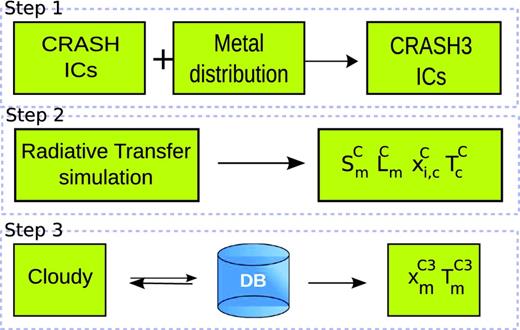
crash3 simulation pipeline. The quantities S, L, xi and T are the SED, luminosity, ionization fractions (per species i) and gas temperature. The subscripts ‘c’ and ‘m’ refer to all the cells in the computational domain and the metal-enriched cells only, while the superscripts C and C3 refer, respectively, to the quantities provided by the RT simulation in Step 2 and by the DB, i.e. as a product of the full crash3 pipeline. See text for more details.
More specifically, crash3 recognizes the metal-enriched subdomain by applying a masking technique to it and by labelling the metal-enriched cells, which are indicated here with the subscript ‘m’. After masking the m cells containing metals, it derives the SED and luminosity of the ionizing radiation present in each of the ‘m’ cells (S, L)m, which are then used to query a dynamic data base (DB) of configurations precomputed with cloudy to identify the corresponding ionization states of the metals and the temperature of the gas. This procedure is repeated for a set of times tk ∈ {t0, …, tf} and the physical state of the enriched cells is then evaluated as a sequence of kf equilibrium configurations at tk. To ensure that the ionization level of the metals is consistent with the energy configuration, the pipeline checks that the ionization fractions of H and He evaluated by cloudy and crash are in agreement. An example of this internal convergence test can be found in Section 5.1.1.
It should be noted that this approach neglects the contribution of metals to the optical depth, as well as to the diffuse radiation emitted by recombining gas. This approximation is justified as long as the metal abundances are very small compared to those of H and He. In fact, when the number density of heavy elements nZ ≳ 10− 3nH, the total photoionization cross-section starts to be dominated by the metal component (see Draine 2011, chapter 13, for a complete discussion). Because the metallicity observed in the IGM is typically below this value (see the Introduction), the above assumption is justified in the cases of our interest.
As detailed in Section 3, cloudy can deal with either a single source configuration or a background radiation. If only a single source is present in the computational domain of crash or when each cell is illuminated from a preferential direction, then the cloudy point source configuration should be used to estimate the ionization and temperature state of the cell. When instead a cell is illuminated more or less uniformly from all directions, then the background radiation setup should be adopted.
In the current implementation of crash3, we have included the species C, O and Si, which are the most abundant metals observed in the IGM (see the Introduction). However, the inclusion of other species, which may be relevant for a more accurate estimate of the gas cooling function, is a straightforward extension of the present scheme (see Section 5.1.5).
Despite the conceptual simplicity of the approach described above, the coupling of crash and cloudy in a single numerical scheme presents several technical challenges. In the following, we will describe in more detail the strategy adopted for such integration and some aspects of the pipeline.
Step 1: initial conditions
The starting point of the pipeline is the setup of the crash3 ICs, which are the same as those of crash as specified in Section 2, with the addition of the spatial distribution and abundance of all the metal species present in the computational domain. These can be artificially created by hand or can be obtained as a result of, for example, hydrodynamic simulations that include physical prescriptions for metal production and spreading.
A preliminary analysis of the spatial distribution of metals allows us to identify the m cells that need to track the radiation field (Step 2) and then query the precomputed DB (Step 3). To identify these cells, a Boolean mask is built isolating the enriched portion of the simulation volume. The building of the mask can be performed before the beginning of the simulation and passed as an additional IC or can be created in memory during the simulation initialization. If the mask contains m true values, a shadow map of ‘m’ cell spectra, SCm, and luminosities, LCm, is allocated to store the shapes and luminosities of the incoming packets: each time a packet enters a cell, the mask is used to check whether the cell is an enriched one and consequently SCm and LCm should be updated (see Step 2). The masking has been designed to optimize the performance of the code, but in principle the SED and luminosity can be calculated in each cell of the computational domain, if required.
Step 2: RT simulation
The next step (Step 2 in Fig. 1) consists of performing a RT simulation which, in addition to the evaluation of (xi, T)Cc in all the cells of the domain, tracks also the SED and luminosity of the ionizing radiation in each of the m metal-enriched cells (S, L)Cm. All the above physical quantities are stored at times tk, as already mentioned above. The values of (S, L)Cm at tk are determined adding up the contribution of all the incoming photon packets up to that time. In practice, the code tracks all the multifrequency packets entering the cell and calculates LCm as the sum of the luminosities of all the packets, while SCm as the average SED in each frequency bin.
Step 3: determination of the physical state of the metal-enriched cells
Finally, a search engine2 looks for the cloudy precomputed configuration that best matches the values of H, He, metal number densities and |$(x_{\rm H {\small II}},x_{{\rm He {\small II}}},x_{{\rm He {\small III}}},S,L)_{\rm m}^{\rm C}(t_k)$|. The best-fitting configuration then provides the ionization fractions of the metal ions and the temperatures TC3m of the gas in the metal-enriched subdomain (Step 3 in Fig. 1).
If the matching criteria are not satisfied (see below and Appendix B for more details), the DB is extended with additional on-the-fly cloudy runs. It is important to point out that Step 3 does not severely affect the basic algorithm performances because it is confined only to the m enriched cells and a large number of cloudy calculations are precomputed and stored in the DB. The interested reader can find more details about the lookup strategy in Appendix B.
In realistic applications, the temperature provided by the hydrodynamics (Thydro) could be significantly higher than the temperature established by the RT. This generally happens in gas-shocked regions where the metal ions are determined mainly by collisional ionization rather than photoionization. Collisional ionization is correctly handled by the pipeline at Step 2 for H and He, because crash selects T = max(TC, Thydro) during its simulation initialization process, maintaining the right temperature. Note that these regions are known as ICs, and a masking technique can be used to isolate them from the standard pipeline workflow. The ionization status of the metal component eventually present in these cells can be determined from cloudy precomputed tables, and by interpolating the gas number density, metallicity, temperature, as well as the ionization fractions of hydrogen and helium. For more details on this technique, see Oppenheimer & Davé (2006), and references therein.
TESTS
In this section, we present three tests designed to establish the reliability of the new code. The first test (Section 5.1) concentrates on the standard Strömgren sphere case, albeit of a metal-enriched gas. The second test (Section 5.2) investigates the sensitivity of crash3 to fluctuations of the radiation field induced by different source types and tracked by the many metal ionization states. Finally, the third test (Section 5.3) describes a more realistic physical configuration by using as ICs those from a snapshot of a hydrodynamic simulation.
Hereafter, the gas metallicity (or equivalently the metal mass fraction) is defined as Zg = MZ/Mg, where MZ is the total mass of the elements with atomic number higher than 2 and Mg is the total mass of the gas; the metal mass fraction in the Sun is set to Z⊙ ≈ 0.0126, according to the metal abundances relative to hydrogen as reported in the cloudy HAZY guide I, and references therein, and taking into account the 10 most abundant elements: H, He, C, N, O, Ne, Si, Mg, S and Fe.
Unless otherwise stated, the metal feedback on the calculation of the gas temperature is neglected and we use kf = 100.
Test 1: Strömgren sphere with metals
We consider a configuration similar to the one in Test 2 of the Cosmological Radiative Transfer Comparison Project (Iliev et al. 2006a), but for the presence of metals.
The simulation box has a comoving side length of 6.6 kpc and it is mapped on to a regular grid of N3c = 1283 cells. The gas is assumed to be uniform and neutral at the initial temperature T = 100 K, with a number density ngas = 0.1 cm−3 and a hydrogen (helium) number fraction of 0.9 (0.1). Only one point source is considered with coordinates (1,1,1), a blackbody spectrum at temperature T = 105 K and ionization rate of |$\skew4\dot{N}=10^{51} \mathrm{photons s}^{-1}$| (i.e. a luminosity |$L\simeq 5\times 10^{40} \rm {erg} \rm {s}^{-1}$|). To ensure a good convergence of the MC scheme, the source radiation field has been sampled by 2 × 10⁸ photon packets. The redshift of the simulation is set at z = 0 and the simulation duration at tf = 5 × 10⁸ yr, i.e. several times the recombination time characteristic of the simulated gas configuration. This choice assures that convergence is reached at the end of the simulation. We uniformly contaminate the gas with carbon (nC ≃ 2.2 × 10⁻⁷ cm−3), oxygen (nO ≃ 4.41 × 10⁻⁷ cm−3) and silicon (nSi ≃ 3.12 × 10⁻⁸ cm−3), corresponding to Zg = 6.45 × 10⁻³ Z⊙. These numbers are obtained maintaining the metal abundances relative to hydrogen mentioned above. Finally, the source spectrum is sampled by 91 frequencies and it extends to an energy Emax = 0.2 keV, in order to include the photoionization edge of the ion O vi.
Although we contaminate the entire box with metals, it is possible to significantly reduce the number of DB queries taking advantage of the spherical geometry of the problem and assuming that each radial direction is equivalent. This is justified as long as the number of photon packets used is large enough that the fluctuations induced by the MC sampling are negligible. We then apply a spherical average of all the relevant physical quantities at each distance d (expressed in cell units) from the ionizing source, and we use these averaged values to search for the better matching configuration in the DB. All the quantities discussed and displayed in this test should be intended as explained above, i.e. as spherically averaged values.
Pipeline convergence
Before proceeding further with the analysis of the results, we discuss the internal convergence of the pipeline. More specifically, we need to assure that the ionization fractions |$x_{\rm H {\small II}}$|, |$x_{\rm He {\small II}}$| and |$x_{\rm He {\small III}}$| calculated in Steps 2 and 3 of the pipeline are in agreement with some user-defined threshold. The same needs to be true for the temperature T if the effect of metals is negligible. This would ensure that the physical configuration and energetic balance evaluated in Steps 2 and 3 are fully consistent. To this aim, we run Test 1 in the absence of heavy elements.
In Fig. 2, we show the profile of |$x_{{\rm H {\small I}}}$|, |$x_{{\rm H {\small II}}}$| (top panel), |$x_{{\rm He {\small I}}}$|, |$x_{{\rm He {\small II}}}$| and |$x_{{\rm He {\small III}}}$| (middle panel) as evaluated by Step 2 (dashed lines and variables with superscript C) and Step 3 (solid lines and variables with superscript C3) at the time tf = 5 × 10⁸ yr. The values of |$x_{\mathrm{H {\small I}}}$| and |$x_{\mathrm{H {\small II}}}$| result in agreement within 10−4 for d < 40 cells (∼2 kpc) and within 10−2 up to the ionization front (I-front), identified as the location where the ionized fraction drops below ∼0.8. The agreement degrades to ∼18 per cent (with respect to the maximum absolute difference between ionization fractions) in the two cells in which the curves of |$x_{{\rm H {\small I}}}$| and |$x_{{\rm H {\small II}}}$| cross, and then it restores up to 10−3. Both codes predict the crossing in the same cell. A similar behaviour is shown in the middle panel for helium. A discrepancy of ∼7 per cent in the |$x_{\rm He {\small II}}$| curves is seen at a distance d ∼ 22 cells, when the abundance of He ii starts to increase. He iii results in an even better agreement, up to 10−4. Reasonable accuracy (less than 20 per cent) is also reached in the fronts of He ii and He i where both algorithms predict a similar shape. Because at the end of the H ii region the intensity of the radiation has dropped substantially (see the following section), sometimes cloudy does not find a convergent solution in few iterations, and this results in a poorer agreement between Steps 2 and 3.
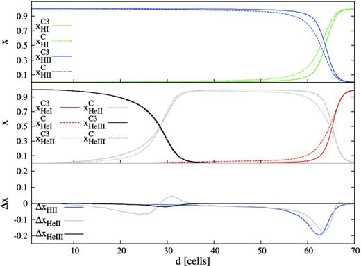
Convergence between Step 2 (dashed lines and variables with superscript C) and Step 3 (solid lines and variables with superscript C3) for Test 1 in the absence of metals (see text for details). The lines refer to the simulation time tf = 5 × 10⁸ yr. At distances larger than 70 cells, the gas is neutral and therefore it is not shown in the plots. Top panel: profile of |$x_{\mathrm{H {\small I}}}$| (green lines) and |$x_{\mathrm{H {\small II}}}$| (blue). Middle panel: same as above for |$x_{\mathrm{He {\small I}}}$| (red lines), |$x_{\mathrm{He {\small II}}}$| (grey) and |$x_{\mathrm{He {\small III}}}$| (black). Bottom panel: Δxi = xCi − xC3i for i = H ii (blue line), He ii (grey line) and He iii (black line).
The above differences are more evident in the bottom panel of the figure, where we show the absolute difference Δxi = xCi − xC3i for i = H ii, He ii and He iii.
Despite the satisfying agreement in the crash3 implementation, some small discrepancies remain due to the differences between the crash and cloudy geometries and the numerical implementation of the ionization and energy equations (see Section 3). We found that a critical ingredient to reach an acceptable convergence is to sample the source spectrum with a large number of frequency bins (see Section 5 for details). This is necessary because the helium component is very sensitive to this sampling, in particular in the vicinity of the ionization potential of He ii.
The temperature radial profiles estimated in the two steps are shown in Fig. 3 (top panel). The curves present large discrepancies in the cells near the source, with a relative variation ΔT/T = (TC3 − TC)/TC3 as high as 60 per cent. The difference drops below 30 per cent for d > 30 cells. This is not reflected in the H and He profiles shown in Fig. 2 because of the weak temperature dependence in the gas recombination coefficients. Such a difference has been already noticed and discussed in the crash versus cloudy comparison test in MCK09 and can be ascribed just to the different implementation of the temperature estimate in the two codes.
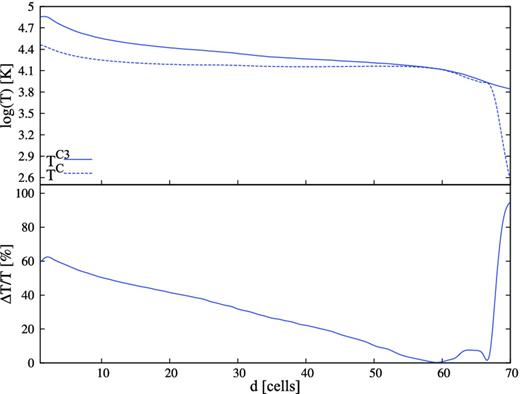
Top panel: temperature convergence between Step 2 (TC, dashed line) and Step 3 (TC3, solid line) for Test 1 in the absence of metals (see text for details). The lines refer to the simulation time tf = 5 × 10⁸ yr. Bottom panel: relative difference ΔT/T = (TC3 − TC)/TC3.
Because crash updates the temperature (compared to its initial value) only in those cells reached by ionizing photons, outside the H ii region T drops to the initial value of 100 K. On the other hand, the temperature calculated by Step 3 is provided by cloudy and, as already mentioned above, all the regions where the intensity of the radiation is too faint do not provide a convergent solution. In the few cells in which cloudy cannot provide a reliable estimate because of the too weak radiation field, the crash temperature TC is retained as a better estimate of the physical temperature at the front.
These convergence tests have been repeated using different ICs for the gas number density and the source luminosity. More specifically, we have run simulations on a grid of cases with values ngas = 1, 0.1, 0.01 cm− 3 and |$\skew4\dot{N} = 5\times 10^{50}, 5\times 10^{51} \rm {photons\ s}^{-1}$|. It is found that, as the gas density decreases, the agreement improves for the H species, while small discrepancies still remaining in the He species. Such discrepancies are, on the other hand, always below 20 per cent and remain limited to the small number of cells encompassing the I-fronts. A similar improvement is observed also for the gas temperature convergence.
Hereafter all the variables will refer to values calculated at Step 3 and the superscript C3 will be omitted to simplify the notation.
Ionization field
In Fig. 4 we show how the spectral shape of the ionizing radiation field described in terms of its spherical average (obtained as described at the beginning of Section 5) changes with the distance d as a result of geometrical dilution and filtering. Each line refers to the simulation time tf = 5 × 10⁸ yr.
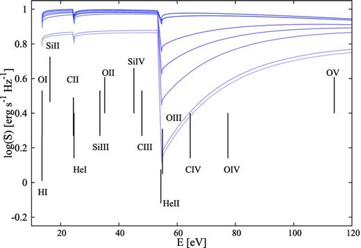
Normalized logarithm of the spherically averaged spectra. The lines refer to the spectra at a distance d (from the top to the bottom) of 20, 27, 38, 45, 55, 69 and 70 cells. The spectra correspond to a time tf = 5 × 10⁸ yr. As a reference, some ionization potentials are also indicated as the vertical lines.
The spectra shown are truncated at E = 120 eV to have a better visualization of the most relevant line potentials. The upper curve corresponds to a distance of d = 20 cells, while the lower to d = 70 cells; at larger distances the intensity of the radiation becomes too faint to solve the ionization equilibrium in every configuration at Step 3 of the crash3 pipeline. Because the medium is fully transparent in H and He up to a distance d = 20 cells, we have normalized the spectra in the figure to the maximum value of the spectrum at d = 20 cells. This choice allows a better visualization of the shaping effects by the partially ionized regions. The ionization potentials of the metals enriching the box (see Table 1) are also shown for reference even if, by design, metals do not contribute to the filtering of the ionizing radiation. The absorption due to H i, He i and He ii is clearly visible corresponding to the respective ionization potentials, i.e. 13.6, 24.6 and 54.4 eV, respectively.
Ionization potentials for H, He, C, O and Si up to the ionization level VI as used in cloudy.
| Eion (eV) | H | He | C | O | Si |
|---|---|---|---|---|---|
| |${E}_{x\rm {{\small I}}}$| | 13.598 | 24.587 | 11.260 | 13.618 | 8.152 |
| |${E}_{x\rm {{\small II}}}$| | 54.400 | 24.383 | 35.118 | 16.346 | |
| |${E}_{x\rm {{\small III}}}$| | 47.888 | 54.936 | 33.493 | ||
| |${E}_{x\rm {{\small IV}}}$| | 64.494 | 77.414 | 45.142 | ||
| |${E}_{x\rm {{\small V}}}$| | 392.090 | 113.900 | 166.770 | ||
| |${E}_{x\rm {{\small VI}}}$| | 489.997 | 138.121 | 205.060 |
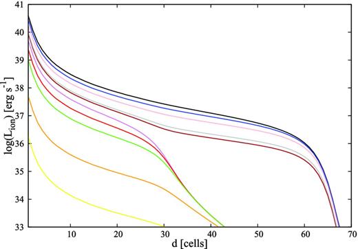
Logarithm of the photoionizing luminosity, Lion, as a function of d at a time tf = 5 × 10⁸ yr. The different curves are calculated integrating all the photons above the ionization threshold of (from the top to the bottom curve): H i (black), He i (blue), Si iii (pink), Si iv (grey), C iii (brown), He ii (violet), C iv (red), O iv (green), O v (orange) and O vi (yellow).
Because the spectrum includes only photons with E > 13.6 eV, Lion is an underestimate for those elements with an ionization potential below 13.6 eV, i.e. carbon and silicon. Note that LOI, |$L_{\mathrm{C {\small II}}}$| and |$L_{\rm O {\small III}}$| overlap, respectively, with |$L_{\rm H {\small I}}$| (black line), |$L_{\mathrm{He {\small I}}}$| (blue line) and |$L_{\rm He {\small II}}$| (violet line) because of the very similar ionization potential. If we increased the frequency resolution of the spectrum, the curves would show some small difference. This would be at the expense of the computational time without significant advantages in the accuracy of the metal ionization state. For this reason, we do not further increase the frequency resolution. Notice that all the luminosities decrease smoothly with d; this is consistent with the behaviour expected in an H ii region, as already reported and extensively commented in Maselli et al. (2003) and MCK09 for the hydrogen and helium components.
Metal ionization states
We now analyse the behaviour of the metal ionization states, plotted in Fig. 6. Before discussing the figure in detail, it is necessary to point out that the balance among the different ions is primarily established by the relative values of their ionization potentials and of their recombination coefficients (see Ferland 2003). It also depends on the spectral distribution of the radiation field and its variations with the distance from the source, as induced by the RT effects. The complex interplay between these numerous processes makes the interpretation of the results non-trivial; despite this, some trends have a straightforward explanation.
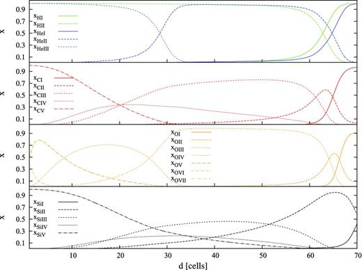
Fractions of the various components as a function of distance d from the source in Test 1. The values are taken at the simulation time tf = 5 × 10⁸ yr. From the top panel to the bottom, the species are: H (green) and He (blue); C (red); O (orange); and Si (black). In each panel, the same ionization states are represented by the same line-styles: solid lines refer to the neutral components (e.g. O i), long-dashed lines to the first ionization state (e.g. O ii), short-dashed lines to the second (e.g. O iii), dotted lines to the third (e.g. O iv), long-dash–dotted lines to the fourth (e.g. O v), short-dash–dotted lines to O vi and dash–spaced lines to O vii.
Because of the small amount of metals included in this test, we expect their impact on the evolution of H and He to be negligible. This is confirmed by a comparison of the curves in the top panel of the figure to the corresponding curves in Fig. 2, which are obtained without metals. The maximum difference is ∼7 per cent across the I-front of H ii. Additional effects on the ionization fractions induced by an increase in the gas metallicity will be investigated in Section 5.1.5.
We now turn to analyse the behaviour of carbon (second panel from the top). For d < 30 cells, C is in the form of C iii, C iv and C v, with a predominance of the latter close to the source. This high ionization level is obtained from a combination of collisional ionization and photoionization. The evolution of C iii is very similar to that of He ii because of the similar ionization potentials (see Fig. 4). The abundance of C iv is dictated by the evolution of C iii and C v, and their relative recombination coefficients. C iv is present throughout the entire H ii region, with |$x_{\mathrm{C {\small IV}}}$| being always below 30 per cent. For d ≳ 30 cells |$x_{\mathrm{C {\small V}}}$| goes to zero because only few C iv ionizing photons are available (see, for reference, Fig. 5). The ionization potential of C v is outside our frequency range (see Table 1) and thus higher ionization states are not present. Because of the paucity of photons with |$E>E_{\mathrm{C {\small III}}}$|, at d > 30 cells only C iii is present in large quantities with |$x_{\mathrm{C {\small III}}}\sim 70$| per cent. At d ∼ 60 cells, similarly to what happens to H ii and He ii, also C iii declines and C ii dominates. Finally, outside the H ii region, only C i is present.
In the third panel from the top, the ions of the oxygen are shown. The ionization potential for O vi is the highest photoionizing energy available in the adopted spectrum. A very small fraction of O vii is in fact present in few cells around the source. It should be noticed that collisional ionization contributes to this fraction for ∼10 per cent at T ≥ 7 × 10⁴ K, which is present when d < 3 cells. The presence of O vi is more evident but it is consistently limited to the inner region of the ionized sphere and decreases rapidly with the distance from the source in favour of lower ionization levels. For d ≳ 30 cells, O iii dominates the ionization balance until it drops in favour of O ii, roughly at the end of the H ii region. As for the other species, outside the H ii region only O i is present.
In the bottom panel, the behaviour of silicon is reported. Si v completely dominates the inner region of the Strömgren sphere, with a long tail extending to d ∼ 55 cells, where it is in equilibrium with lower ionization states. In the central region, many ions are in equilibrium with a low ionization fraction. Si iii reaches a maximum fraction of ∼0.4 at the centre of the H ii region. Si ii dominates at d > 52 cells. The abundance of Si i in the outskirts of the H ii region is much lower than the one of, for example, C i because of the lower number density of Si and the much larger cross-section of Si i at the resonance (see fig. 13.2 of Draine 2011).
In general, it is possible to say that in the vicinity of the source the most abundant species are those with the higher ionization state compatible with the maximum potential in the spectrum, i.e. H ii, He iii, C v, O v and Si v. Despite |$E_{{\rm O {\small V}}}$|, |$E_{{\rm O {\small VI}}}$| and |$E_{{\rm Si {\small V}}}$| being covered by the spectrum, the abundance of photons at these energies is so low that |$x_{{\rm O {\small VI}}}$|, |$x_{{\rm O {\small VII}}}$| and |$x_{\rm {Si {\small VI}}}$| are negligible. As the distance increases, the luminosity available for ionization decreases, in particular for ions with high ionization potentials (see Fig. 5). This is reflected by the decrease of the abundance of these highly ionization states and the predominance of lower ionization states (e.g. He ii, C iii, O iii and Si iii). Species like Si iv and C iv are always present, although they are not dominant, because the spectrum of the ionizing radiation maintains energies higher than |$E_{{\rm Si {\small III}}}$| and |$E_{{\rm C {\small III}}}$| throughout the H ii region (see Fig. 5). At even larger distances (d > 60 cells), the dominant species are typically singly ionized metals and the neutral components, due to the absence of ionizing radiation.
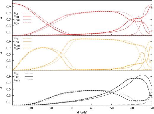
While the discussion above refers to the final gas configuration, in Fig. 7 we show some reference species at different simulation times, i.e. t = 106, 107 and 5 × 10⁸ yr. It should be kept in mind that in this case no metal feedback is included in the calculation (see Section 5.1.5) and thus the profiles of the metal species at each time are independent of each other. While the shape of each species changes substantially between 106 and 107 yr, for t ≳ 107 yr they have almost converged. This is especially true for the metal ionization potentials larger than the third state and for He iii. Overall, the comments made for Fig. 6 at tf = 5 × 10⁸ yr apply also at earlier times.
Fractions of the various components as a function of the distance d from the source in Test 1. From the top panel to the bottom, the species are: H and He, C, O and Si. In each panel, the colours refer to different simulation times: t = 106 (blue), 107 (red) and 5 × 10⁸ yr (black).
Effect of photons with E < 13.6 eV
In this section, we discuss the impact of photons with E < 13.6 eV in the evaluation of metal ionization states. Because the ionization potential of C i and Si i is below |$E_{\mathrm{H {\small I}}}$|, i.e. in a range which is not covered by crash and where the spectrum is set by default to zero, this means that photoionization by photons with E < 13.6 eV is neglected, resulting in a systematic underestimate of |$x_{\mathrm{C {\small II}}}$| and |$x_{\mathrm{Si {\small II}}}$| as visible in the outer region of the Strömgren sphere.
To investigate this limitation of our pipeline, we have extended the spectrum to a lower energy of |$E_{\rm {Si {\small I}}} = 8.152$| eV. It should be kept in mind, though, that in the range |$E_{{\rm Si {\small I}}}$|–|$E_{{\rm H {\small I}}}$| the luminosity of the spectrum is overestimated because the absorption by metals (the only species contributing to the optical depth in this energy range) is not accounted for. This means that the change in the spectrum at these frequencies is due only to geometrical dilution. The approximation is more severe beyond the He ii front (see Fig. 6), where the only surviving radiation has energy below |$E_{\mathrm{H {\small I}}}$| and the optical depth of the medium is dominated by the metals.3
In Fig. 8, we summarize the results of this run by showing the evolution of different C, O and Si ions. The lines with crosses refer to the case in which the source spectrum extends below 13.6 eV. In the inner part of the H ii region, the agreement between the curves with and without the inclusion of the low-energy tail is excellent for the neutral fractions and the first ionization state, while it gets worse for higher ionization states. The reason is that, when the spectrum is extended below 13.6 eV additional physical processes become relevant, in particular line emission from collisional excitation. The most prominent case is the collisional excitation of the O iv line. While the behaviour of xOV is the same in both cases (and for this reason it is not reported here), in the presence of non-H i-ionizing radiation O iv recombines more quickly to O iii, inducing the discrepancies observed between ∼20–35 cells. Something similar happens to C v and C iii, while C iv is not affected because it is not a dominant species at these distances, as shown in Fig. 6. For Si the differences are smaller. The picture in the outskirts of the H ii region instead changes completely: not only do |$x_{\mathrm{C {\small II}}}$|, |$x_{\rm O {\small II}}$| and |$x_{\mathrm{Si {\small II}}}$| extend outside the H ii region, while the corresponding neutral components disappear, but also the higher ionization states are affected. This results from a combination of the photoionization due to the photons with energies below 13.6 eV and the additional physical processes mentioned above. At these distances, the former effect has a larger impact than in the vicinity of the source, where ionization is dominated by photons with energies above 13.6 eV. It should be noted that outside the H ii regions, or, more correctly, when the absorption of photons is not dominated any more by H and He, our assumption of neglecting the metal contribution to the optical depth fails and the metal ionization states are not calculated correctly any more.4
Fractions of C (upper panel), O (middle panel) and Si (lower panel) ions as a function of the distance d from the source in Test 1. In each panel, the lines with crosses refer to Test 1 with the source spectrum extending to a lower ionizing energy of |$E_{\mathrm{Si {\small I}}}$|, rather than |$E_{\rm H {\small I}}$|. Note that the neutral fractions in the former case are equal to zero in the range of cells shown here.
Feedback by metals
In this section, we investigate the effect of metals on the evaluation of the gas temperature. In Appendix A, the convergence of this feedback with respect to the choice of kf is investigated. This is done by calculating T at the time tf = 5 × 10⁸ yr in the standard configuration of Test 1 and then changing the metallicity of the gas.
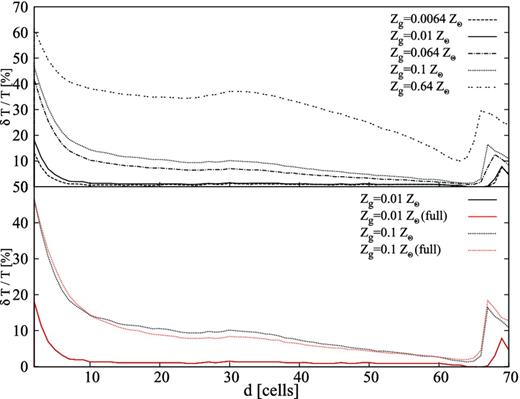
ΔT/T = (T(0) − T(Zg))/T(0) as a function of the distance d from the source in Test 1 at the simulation time tf = 5 × 10⁸ yr (see text for more details). Upper panel: the curves refer to a gas enriched by C, O and Si, and a metallicity Zg of: 0.0064 Z⊙ (dashed line, reference value), 0.01 Z⊙ (solid line), 0.064 Z⊙ (dot–dashed line), 0.1 Z⊙ (dotted line) and 0.64 Z⊙ (dash–spaced line). Lower panel: the curves refer to a gas enriched only with C, O and Si (black lines) or with the 10 most abundant elements in the solar composition (red lines). For both cases, the gas metallicity Zg is 0.01 Z⊙ (solid lines) and 0.1 Z⊙ (dotted lines).
Even if it is not shown in Fig. 9, we have computed the solar and supersolar cases (Zg ≥ 1 Z⊙), finding a deviation of ΔT/T > 50 per cent in the inner region, and values exceeding 40 per cent up to d ∼ 45 cells. These results confirm the dominant role played by metal cooling in this metallicity range. These cases though should be considered only as indicative because in this metallicity regime the metal contribution to the absorption cannot be neglected and the assumptions of our method fail.
As a second step we have investigated the dependence of our results on the gas composition; this is shown in the bottom panel of Fig. 9. More specifically, while the black lines are the equivalent of the ones in the upper panel, the red lines have been obtained including the 10 most abundant elements in the solar composition. Note that the red and black lines are not distinguishable in the reference metallicity case. In both cases, the number densities of metals are such that their abundance relative to H is the same as those in the solar composition. It is clear that, at a fixed metallicity,
the contribution of C, O and Si to the cooling is dominant compared to other elements, such as N, Ne, Mg, S and Fe. We have thus neglected such elements in all further tests. It should be noted that just adding the contribution of N, Ne, Mg, S and Fe to the gas metallicity (without keeping it constant) would bring Zg from, for example, 0.0064 to 0.01 Z⊙ and 0.064 to 0.1 Z⊙.
In Fig. 10, we finally report the effect of a varying metallicity and chemical composition on the ionization fraction of C iv. It is clear that it is safe to neglect metals other than C, O and Si as their impact on the global ionization equilibrium is limited at a maximum of few per cent for Zg ≳ 0.1 Z⊙, while it is close to zero for lower metallicity. A similar effect is observed for all the other relevant ions. On the other hand, the dependence on the gas metallicity Zg is higher and it changes for the various species. In some cases, like the one shown in the figure (as well as O iii and Si iv), the ionization fraction of the species increases with increasing metallicity, while in others (e.g. C iii, O v and Si iv) the trend is reversed. It is beyond the scope of this paper though to discuss this issue in more details.
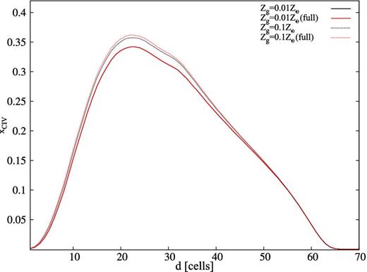
Fraction of C iv as a function of the distance d from the source in Test 1 at the simulation time tf = 5 × 10⁸ yr. The curves refer to a gas enriched only with C, O and Si (black lines) or with the 10 most abundant elements in the solar composition (red). For both cases, the gas metallicity Zg is 0.01 Z⊙ (solid lines) and 0.1 Z⊙ (dotted lines).
Test 2: metal fluctuations in the overlap of two H ii regions
Here we study the behaviour of metals in the H ii region overlap produced by two point sources located in the cells (20, 64, 64) and (40, 64, 64). This geometrical setup is sketched in Fig. 11 and it is designed to investigate the sensitivity of our method to small changes in the source characteristics. This is done by varying the source ionizing rates, |$\skew4\dot{N}_{1}$| and |$\skew4\dot{N}_{2}$|, and their associated blackbody spectral temperatures, T1 and T2. All the other numbers are the same as those in Test 1, with the exception of the gas number density which is ngas = 1 cm−3, to obtain a sharper overlap profile. Because in this test we are interested in studying the behaviour of metals only in the overlap region, we concentrate on the plane corresponding to x = 30 (blue circle in Fig. 11).
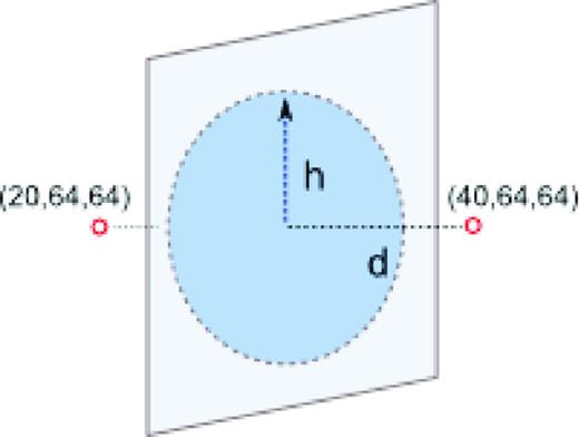
Sketch of the geometrical setup used for Test 2.
Reference case
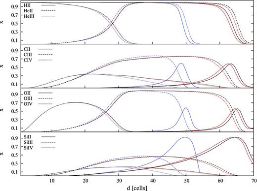
We first describe the setup used as a reference case, with two identical sources with |$\skew4\dot{N}_{1} = \skew4\dot{N}_{2} = 9 \times 10^{51}$| photons s−1 and T1 = T2 = 105 K. Similarly to Test 1, here we show the results by averaging the input physical quantities on all the cells of the plane at the same distance h from the cell (30, 64, 64) (see Fig. 11). The results refer to the final time tf = 5 × 10⁸ yr. Fig. 12 shows the profiles of the ionization fraction of some selected ions.
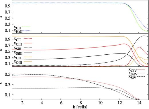
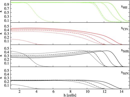
Ionization fractions as a function of h, evaluated in the plane equidistant from the two sources (x = 30) of Test 2 in the reference case. From the top to bottom, the panels refer to: |$x_{\mathrm{H {\small II}}}$| (green dashed line) and |$x_{\mathrm{He {\small II}}}$| (blue dashed line); |$x_{\mathrm{C {\small II}}}$| (red dashed line), |$x_{\mathrm{C {\small III}}}$| (red solid line), |$x_{\mathrm{Si {\small II}}}$| (black dashed line), |$x_{\mathrm{Si {\small III}}}$| (black solid line), |$x_{\mathrm{O {\small II}}}$| (orange dashed line) and |$x_{\mathrm{O {\small III}}}$| (orange solid line); |$x_{\mathrm{C {\small IV}}}$| (red dotted line), |$x_{\mathrm{Si {\small IV}}}$| (black dotted line) and |$x_{\mathrm{Si {\small V}}}$| (black dot–dashed line).
The profile of the H and He species is very similar to that of a single Strömgren sphere (see Test 1), with the exception of |$x_{\mathrm{He {\small III}}}$|, which is always confined to regions very close to the sources and thus is not shown.
In the middle panel, C ii, C iii, Si ii, Si iii, O ii and O iii are shown together because they trace the external regions of the two overlapping Strömgren spheres (see Fig. 6). C iii, O iii and Si iii are present for h < 12 cells with different ionization fractions (|$x_{\mathrm{O {\small III}}}\sim 1$|, |$x_{\mathrm{C {\small III}}}\sim 0.5$| and |$x_{\rm {Si {\small III}}}\sim 0.3$|), indicating that these ions have a different sensitivity to the ionizing field; this is also in qualitative agreement with the relative trends noticed in Test 1 (see Fig. 6).
In the lower panel, |$x_{\rm C {\small IV}}$|, |$x_{\rm Si {\small IV}}$| and |$x_{\rm Si {\small V}}$| are shown. Similarly to the species analysed in the previous panel, they present an almost constant value throughout the fully ionized region, with the exception of |$x_{\rm Si {\small V}}$|, which starts declining earlier, in favour of lower ionization states. The absence of O iv, O v and C v (which reach an ionization fraction of only a few per cent) is consistent with the absence of He iii. Compared to the corresponding species in Test 1, here the ionization fractions are higher due to the larger ionization rate.
Variations in the source ionization rates
In this section, we discuss the variations in the results induced by changes in the ionization rates. These are shown in Fig. 13 for some reference species.
Ionization fractions as a function of h, evaluated in the plane equidistant from the two sources (x = 30) of Test 2 when the source ionization rate is changed compared to the reference case (see text for details). From the top to the bottom, the panels refer to |$x_{\mathrm{H {\small II}}}$|, |$x_{\mathrm{C {\small IV}}}$|, |$x_{\mathrm{Si {\small III}}}$| and |$x_{\mathrm{Si {\small IV}}}$|. In all panels, the solid lines refer to the reference case with |$\skew4\dot{N}_{1} = \skew4\dot{N}_{2} = 9 \times 10^{51}$| photons s−1; dashed lines to |$\skew4\dot{N}_{1} = 9 \times 10^{51}$| photons s−1 and |$\skew4\dot{N}_{2} = 7 \times 10^{51}$| photons s−1; short-dashed lines to |$\skew4\dot{N}_{1} = 9 \times 10^{51}$| photons s−1 and |$\skew4\dot{N}_{2} = 3 \times 10^{51}$| photons s−1; dot–dashed lines to |$\skew4\dot{N}_{1} = \skew4\dot{N}_{2} = 7 \times 10^{51}$| photons s−1; dotted lines to |$\skew4\dot{N}_{1} = \skew4\dot{N}_{2} = 3 \times 10^{51}$| photons s−1.
First, we have decreased the ionization rates of the two sources simultaneously, maintaining the symmetry of the problem, i.e. using |$\skew4\dot{N}_1 = \skew4\dot{N}_2 = 7\times 10^{51}$| and 3 × 1051 photons s−1, the latter being the minimum ionizing rate allowing for an overlap of the two H ii regions. We have then decreased the ionization rate of only one source, while maintaining |$\skew4\dot{N}_{1} = 9 \times 10^{51}$| photons s−1. As expected, the extent of the fully ionized region (upper panel) decreases with decreasing total ionization rate. A similar trend is observed also in the profile of the other species, which changes smoothly with decreasing ionization rate. Compared to the behaviour of |$x_{\rm H {\small II}}$| though, these differ in that also the amount of ionization decreases. Remarkably, |$x_{\mathrm{Si {\small IV}}}$| seems to be insensitive to small variations of the ionization rates, at least in the inner parts of the H ii region. This suggests that other species would be more suitable to give indications on the characteristics of the sources.
By comparing qualitatively the results with those in Fig. 6 we can conclude that crash3 produces the predictable behaviour for the ions also when more than one source is present and that it is sensitive to small changes in the source ionization rates. This is very important for realistic applications of the code.
Variations in the source spectra
In this section, we study the variations induced by changes in the temperatures T1 and T2 of the blackbody spectra. The source ionization rates are set to the reference value |$\skew4\dot{N}_{1} = \skew4\dot{N}_{2} = 9\times 10^{51} \mathrm{photons s}^{-1}$|. The results in terms of distribution of some reference ionization fractions are shown in Fig. 14.
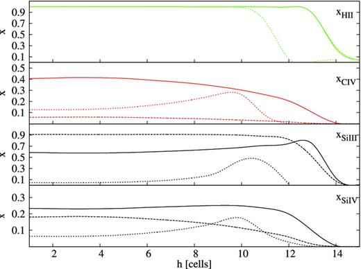
Ionization fractions as a function of h, evaluated in the plane equidistant from the two sources (x = 30) of Test 2 when the source spectrum is changed compared to the reference case (see text for details). From the top to the bottom, the panels refer to |$x_{\mathrm{H {\small II}}}$|, |$x_{\mathrm{C {\small IV}}}$|, |$x_{\mathrm{Si {\small III}}}$| and |$x_{\mathrm{Si {\small IV}}}$|. In all panels, the solid lines refer to the reference case with T1 = T2 = 105 K, the dashed lines to T1 = T2 = 5 × 10⁴ K and the short-dashed lines to T1 = T2 = 5 × 10⁵ K.
In the top panel, the H ii I-front is identical in the cases T1 = T2 = 5 × 10⁴ K and T1 = T2 = 105 K, while it recedes significantly for T1 = T2 = 5 × 10⁵ K. This is because by increasing the temperature from 5 × 10⁴ to 105 K, most of the photons still have |$E<E_{\rm He {\small II}}$| and get preferentially absorbed by hydrogen because of its higher abundance. For these two cases, |$x_{\rm He {\small II}}$| (which is not plotted here) has a profile very similar to that of |$x_{\rm H {\small II}}$|, with the only difference that it slightly increases with increasing temperature because more photons have |$E>E_{\rm He {\small I}}$|. On the other hand, when the temperature of the blackbody spectra is increased to 5 × 10⁵ K, most of the photons have an energy in the vicinity of |$E_{\rm He {\small II}}$|, causing a drop in |$x_{\rm H {\small II}}$| and |$x_{\rm He {\small II}}$| and the appearance of |$x_{\rm He {\small III}}$| (which is not plotted here), which was missing in the other cases, being relegated only in the immediate surroundings of the sources.
While for T1 = T2 = 5 × 10⁴ K there is hardly any C iv available because of the lack of enough photons with |$E>E_{\rm C {\small III}}$|, as the spectrum temperature increases so does |$x_{\mathrm{C {\small IV}}}$|. Increasing the blackbody temperature further, and thus shifting the peak of the blackbody spectrum to higher frequencies, brings a drop in |$x_{\mathrm{C {\small IV}}}$|, which is balanced by an equal increment of |$x_{\mathrm{C {\small V}}}$| (which is not shown in this plot).
Unlike in the previous tests, in this case both Si iii and Si iv show remarkable changes by varying the spectrum temperature. While |$x_{\rm Si {\small III}}$| keeps decreasing as the temperature increases and higher ionization states are favoured, |$x_{\rm Si {\small IV}}$| increases from T1 = T2 = 5 × 10⁴ to T1 = T2 = 105 K, while it decreases when T1 = T2 = 5 × 10⁵ K, similarly to |$x_{\rm C {\small IV}}$|.
Also in this case we can conclude that crash3 is very sensitive to changes in the spectrum of the ionizing sources.
We have verified that a similar conclusion applies when only one of the two source temperatures is changed or when we have adopted a power law rather than a blackbody spectrum.
Test 3: RT on a cosmological density field enriched by metals
In this section, we present an extension of Test 4 proposed in the Cosmological Radiative Transfer Comparison Project (Iliev et al. 2006a). The original test setup has been adopted, but we have extended the ICs to include He, C, O and Si. For reference, the box size is Lb = 0.5 h−1 Mpc comoving, h = 0.72, Nc = 128, the simulation duration is set to tf = 4 × 10⁵ yr, starting at redshift z = 9. The cosmological evolution of the box is disabled and the simulation starts with a neutral gas at an initial temperature T = 100 K.
The H and He fractions are the same as in Test 1. 16 point sources are present in the box with a blackbody spectrum at T = 105 K. The sampling of the spectrum is done with 91 frequencies, to reach the accuracy established in our Test 1. Finally, we have used 108 packets to ensure a good convergence as done in MCK09. It is important to note that the aim of this test is to show how the crash3 pipeline is applied to a realistic density configuration and the rich set of information provided by it, and it is not meant to quantitatively reproduce observational results.
Differently from the previous tests in which we populated the full computational volume with metals, here we assign a metallicity of Zg = Δ × 0.0064 Z⊙ to those cells with an overdensity Δ = ρ/〈ρ〉 > 10. This results in about 5 per cent of metal-enriched cells. The number density of C, O and Si relative to hydrogen is the same as introduced at the beginning of Section 5.
In Fig. 15, the distribution of the C i number density is shown in the slice of the simulation box containing the brightest source, located within the densest region in the computational volume. The distribution of Si i and O i is the same, with |$n_{{\rm Si {\small I}}} = 0.142\times n_{{\rm C {\small I}}}$| and |$n_{{\rm O {\small I}}} = 2\times n_{{\rm C {\small I}}}$|. By construction, most of the metals are concentrated in the vicinity of the sources and in general in the highest density regions.

Slice cut through the simulation box showing the initial distribution of |$\log (n_{\mathrm{C {\small I}}}) (\mathrm{cm}^{-3})$| in Test 3.
As shown in Fig. 9, gas with metallicity Zg > 0.1 Z⊙ starts to cool with different efficiency depending on the distance from the illuminating source (see the comments in the Section 5.1.5), while for Zg > 0.64 Z⊙ the cooling is relevant at every distance from the source. In the box of this test, cells with Δ > 100 are only 0.012 per cent of the total number, while cells with Δ > 50 are about 4 per cent. We then expect the effect of metal cooling to be negligible on the global ionization status of the medium and we ignore it in discussing the results. In realistic 3D simulations, the metal cooling should be carefully accounted for in all the cells with Zg > 0.1 Z⊙, because it acts differently depending on the gas metallicity and the RT effects shaping the field. The statistical effects of the metal cooling will be analysed with care in future applications in the context of physically motivated enrichment patterns.
To better understand the distribution of the metal ionization species discussed in the following, in Fig. 16 we show the distribution of gas temperature in the same slice as above at a time t = 5 × 10⁴ yr. The black regions (T ∼ 100 K) correspond to areas not reached by the radiation field, the green colour clearly traces the He ii I-fronts at a typical temperature T ∼ 2 × 10⁴ K, while the red/orange is associated with regions at T ∼ 4 × 10⁴ K, dominated by H ii and He ii. Finally, the warmer, yellow regions correspond to areas where there is also substantial He iii.
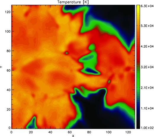
Slice cut through the simulation box showing the distribution of the gas temperature T in the same slice of Fig. 15 at the time t = 5 × 10⁴ yr in Test 3.
The distribution of some reference metal species is shown in Fig. 17 across the same slice. While in the vicinity of the brightest source C v is present in large quantities, with |$x_{\rm C {\small V}}$| as high as 1, only small traces are visible farther away. On the other hand, these regions are typically rich in C iii, showing a qualitative behaviour similar to the one discussed in Test 1, where C v and C iii are complementary species. Consistently with the same Test 1, C iv is present everywhere along the filaments with relatively low abundances. Regions with fractions close to zero are those which have not been reached by ionizing radiation (see Fig. 16). A similar behaviour is observed for O, with O v present in very small traces only in the vicinity of the brightest source, O iv extending a bit farther away along the filaments and O iii being present in substantial amounts elsewhere. Finally, while there are only traces of Si iv, |$x_{\rm S {\small IV}}$| is as high as 1 in the vicinity of the source and Si iii is present in modest quantities everywhere.
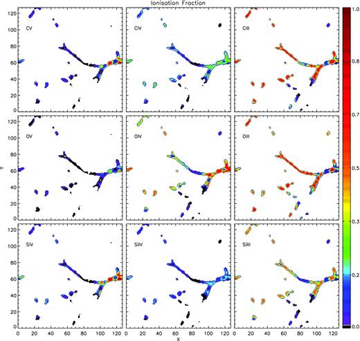
Slice cut through the simulation box showing the distribution of (from the left-hand to right-hand side and from the top to bottom): |$x_{\rm C {\small V}}$|, |$x_{\rm C {\small IV}}$|, |$x_{\rm C {\small III}}$|, |$x_{\rm O {\small V}}$|, |$x_{\rm O {\small IV}}$|, |$x_{\rm O {\small III}}$|, |$x_{\rm S {\small IV}}$|, |$x_{\rm Si {\small IV}}$| and |$x_{\rm Si {\small III}}$|. The slice shown is the same as of the previous figures at the time t = 5 × 10⁴ yr in Test 3.
While it is not possible to make a quantitative comparison with Test 1, the qualitative results in terms of ionization fractions at a given distance from the brightest source are in good agreement, with the highest ionization levels present only in the close proximity of the source and the lower ionization levels present everywhere along the filaments hit by the ionizing radiation.
Similarly to what done in Section 5.1.4, we have investigated the impact on the evaluation of metal ionization states of photons with E < 13.6 eV by extending the spectrum to energies lower than 13.6 eV down to |$E_{\rm Si {\small I}}$|. In Fig. 18, the differences in ionization fractions (|$\Delta x_i = x_{i,E_{\rm Si {\small I}}}-x_{i,E_{\rm H {\small I}}}$|) computed in the two setups are reported for the same ions of Fig. 17. As for Test 1, we find that where |$x_{\rm H {\small II}} \sim 1$| the agreement between the cases with and without the inclusion of the low-energy tail is excellent in most of the metal-enriched domain. xOIV and |$x_{\rm O {\small III}}$| present an average discrepancy of about 13 per cent, with a maximum of ∼40 per cent confined to few cells where the ionization fractions are relatively low (i.e. below ∼30 per cent). For higher x the agreement is excellent, reflecting the results in Section 5.1.4, where the largest discrepancies were observed corresponding to those cells in which the abundance of the different species was raising or declining. On the other hand, xOV always shows a good agreement between the two cases. The Si and C ionization fractions present a maximum discrepancy below 10 per cent for their higher (i.e. iv and v) ionization species, while it raises to ∼40 per cent for |$x_{\rm C {\small III}}$| and |$x_{\rm Si {\small III}}$|. Also for these species only few cells have such large discrepancies.
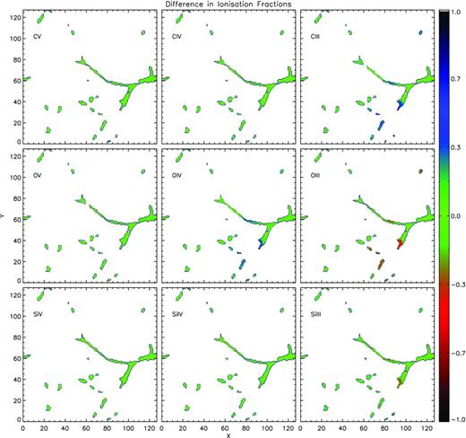
Slice cut through the simulation box showing the distribution of the differences in ionization fractions obtained in Test 3 with the reference source spectrum and with a spectrum extending to a lower ionizing energy of |$E_{\rm Si {\small I}}$| (|$\Delta x_i = x_{i, E_{\rm Si {\small I}}} - x_{i, E_{\rm H {\small I}}}$|; see text for more details). From the left-hand to right-hand side and from the top to bottom, the panels refer to the species: C v, C iv, C iii, O v, O iv, O iii, Si v, Si iv and Si iii. The slice shown is the same as of the previous figures at the time t = 5 × 10⁴ yr.
In general, we can conclude that, similarly to what seen in Test 1, the extension of the spectrum to energies lower than 13.6 eV results in some discrepancies in the evaluation of the metal ionization fractions. Such discrepancies are limited to some of the metal ions (especially the lowest ionization states) and are largely due to a number of physical processes that are neglected (see the footnote of the Test 1 section and the discussion in Section 5.1.4). In the selected slice, they are also confined to a small number of cells typically located far from the ionizing sources. As a reference, the percentage of metal-enriched cells that present a discrepancy larger than 5, 10, 25 and 50 per cent in the visualized species is 19.3, 9.6, 4.2 and 0.6 per cent, respectively.
CONCLUSIONS
In this paper, we presented crash3, the latest release of the 3D RT code crash. In its current implementation, crash3 integrates into the reference algorithm the code cloudy to evaluate the ionization states of metals, self-consistently with the RT through the most abundant species, i.e. H and He. The feedback of the heavy elements on the calculation of the gas temperature is also taken into account, making crash3 the first 3D code for cosmological applications which treats self-consistently the RT through an inhomogeneous distribution of metal-enriched gas with an arbitrary number of point sources and/or background radiation. It should be noted that the algorithm is based on the assumption that metals do not contribute to the gas optical depth, which is valid in typical configurations of cosmological interest, e.g. in the IGM. On the other hand, the code is not suitable for applications in which metallicities ≳ Z⊙ are involved.
The pipeline has been tested in idealized configurations, such as the classic Strömgren sphere, albeit enriched with heavy elements, as well as in a more realistic case of multiple sources embedded in a polluted cosmic web, which shows the rich set of information provided by the metal ionization states. Through these validation tests, the new method has been proved to be numerically stable and convergent with respect to a number of parameters.
The dependence of the results on, for example, the source characteristics (spectral range and shape, intensity), the metal composition, the gas number density and metallicity has been investigated. Despite the difficulty in testing quantitatively the results, we find that the qualitative behaviour is consistent with our expectations.
In conclusion, crash3 is an excellent code to simulate the evolution of various species in a low-metallicity gas illuminated by ionizing radiation, which can be modelled both as background radiation and point sources. crash3 will then be an invaluable tool to investigate the interpretation of, for example, metal absorption lines in QSOs’ spectra or fluctuations in the UV background, in more detail, with a better modelling of the relevant physical processes and with a higher accuracy than done before. These applications are topics for further investigations.
The authors would like to thank the referee, Alexey Razoumov, for his very constructive comments. The authors are also grateful to J. Bolton, R. Davé, A. Ferrara and J. Ostriker for enlightening discussions. AM acknowledges the support of the DFG Priority Program 1177. LG acknowledges the support of the DFG Priority Program 1573.
We have implemented a Standard Query Language DB using one of the codes freely available to the scientific community. More details can be found in Appendix B.
In realistic configurations, other absorbers like dust and molecules could play a dominant role in establishing the optical depth of the medium at these frequencies, but these are not accounted for in crash3.
Other important processes playing a relevant role in the outskirts of the H ii region, e.g. O+ + H ↔ O + H+, have been deactivated in cloudy by disabling the charge transfer. More references on the subject can be found in Draine (2011).
REFERENCES
CONVERGENCE TESTS
When the temperature feedback is introduced in the crash3 pipeline (see the description of Step 3) kf times, the RT process is altered. While the gas recombination depends weakly on the temperature and we can expect negligible effects, the numerical convergence of the metal ionization fractions needs to be verified for different values of kf. Here we show the results of some tests run to check the convergence of our results with respect to kf when the metal feedback is enabled.
In Fig. A1, we show the profile of the variation of the reference ionization fraction (|$x_{\rm C {\small II}}$|) and temperature for Test 1 run with the metal feedback switched on. The lines refer to the final time tf = 5 × 10⁸ yr and to the values of kf = 10, 50, 100 and 500. The convergence of the results within the ionized sphere (d ≤ 40 cells) is excellent: even for small values of kf the relative discrepancies remain within few per cent both in the ionization fraction (top panel) and in the temperature (bottom panel). Numerical oscillations of a few per cent (or smaller) in Δx/x are present in a handful of isolated cells, but they disappear for kf ≥ 100.
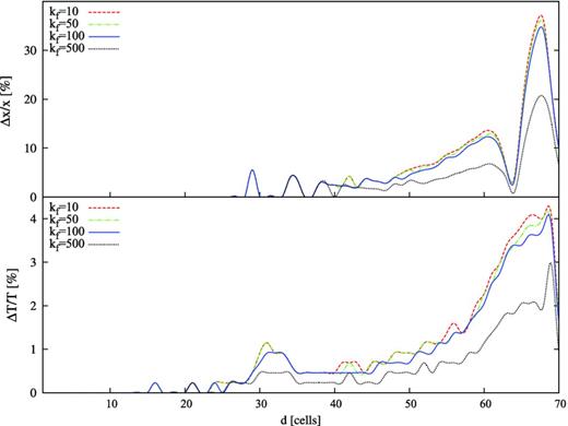
Δx/x = ∣x(kf = 1000) − x(kf)∣/x(kf = 1000) (upper panel) and ΔT/T = ∣T(kf = 1000) − T(kf)∣/T(kf = 1000) (lower panel) as a function of the distance d from the source in Test 1 including the feedback from metals. Here x refers to the ionization fraction |$x_{\rm C {\small II}}$|. The curves are plotted at the time tf = 5 × 10⁸ yr and refer to a value of kf = 10 (red dashed lines), 50 (green dot–dashed lines), 100 (blue solid lines) and 500 (black dotted lines).
Closer to the I-front (d ≥ 50), where |$x_{\rm C {\small II}}$| is very small (i.e. ≤10−4), the convergence is worse, in particular in the two to three cells encompassing the I-front. This behaviour was expected because, as already discussed in Test 1, the accuracy of our scheme is diminished in the outer regions of the ionized bubble, where the cloudy computation is not always convergent. It should be noticed, however, that |$x_{\rm C {\small II}}$| presents one of the worse behaviours and higher ionization states are more numerically stable. We have checked that the convergence is similar also at earlier times, when the ionized sphere has not reached an equilibrium configuration. Other species show a similar dependence on kf. For example, |$x_{\rm C {\small IV}}$| presents an excellent convergence (of the order of a per cent) within the ionized region already with kf = 10, while in the proximity of the I-front, where |$x_{\rm C {\small IV}} \le 10^{-6}$|, it degrades to tens of per cent.
The temperature shows an even better behaviour, with a relative convergence of a few per cent even in the vicinity of the I-front. Also at earlier times the convergence is never worse than 10 per cent. The oscillations in the curves have the same origin as those in the upper panel.
We should notice that the value of kf needed to reach a good convergence is likely dependent on the problem at hand. In general, though, we can conclude that we expect a value of kf ∼ 500 to be sufficient for most applications which require the feedback of metals on the determination of the gas temperature.
DATA BASE IMPLEMENTATION AND LOOKUP STRATEGY
Here we provide more details on the implementation of the relational DB introduced in Section 4 and the lookup strategy we use to query its data.
Note that Ncomp depends indirectly on the adopted grid resolution Nc and the metal filling factor; therefore, the size of the metal map Nm can rapidly reach a high value. For instance, a simulation with Nc = 1283, Nm ∼ 105 (i.e. cell filling factor of 5 per cent) and tf = 10 requires Ncomp ∼ 106 computations in a single snapshot. As the direct evaluation of Ncompcloudy runs during the RT simulation is feasible just in few cases, we use a DB of precomputed configurations to alleviate the total computational cost.
The DB stores a large number of cloudy runs abstracted as object data associating ICs (RUN_ICs) with the resulting ionization fraction and temperature (RUN_RESULTS); this association is uniquely identified by an indexing key (RUN_ID).
The set of RUN_ICs is composed by the number densities of all the species nm polluting the metal-contaminated sub-domain, the luminosity Lm and the spectral shape Sm, specified on a fixed number of frequency bins (see Section 4). As detailed in Section 5, 91 bins are generally required to obtain the accuracy of the tests in matching the H ii fronts.
The RUN_RESULTS set is composed by the ionization fractions of all the species xC3m and the temperature TC3.
As prescribed by the relational DB theory, all the variables are organized in columns of the DB tables and related by RUN_ID. The DB solution is practically implemented by combining two relational DBs: a reduced ‘in-memory DB’ (called production DB) used during the RT (see Step 3 of the pipeline in Section 4.3), and an ‘archiving DB’ (a standard TCP/IP accessible DB) collecting the results of many runs and increasing in time. Before running a simulation, the content of the smaller DB is extracted from the archiving DB and customized on the problem at hand as explained below.
The content of the production DB can be tuned on the specific problem under investigation because the crash3 pipeline is applied in post-processing and part of the RUN_ICs can be partially pre-constrained. First, the nm values are exactly known from the hydro-simulation at fixed redshift, while the values of Lm and Sm can be only predicted because they are affected by the metal feedback. Secondly, in the regime of applicability of our pipeline, we tested that the metal cooling feedback is weak on the RT field and by running a RT simulation just through H and He (the only absorbers; see Section 4) we can have a reasonable estimate of the statistics of the produced spectral shapes. Note also that in the absence of feedback from metals, Lm and Sm are provided exactly from Step 2 at every time but Ncomp can be huge and still requires some precomputed configurations to successfully finish the run.
The DB is then populated by spanning a subset of compatible ICs providing a non-redundant set of final ionization fractions and temperatures; this is realized by testing the sensitivity of the photoionization software to small variations (δn, δL, δS) of their values. An example of these tests is reported in Section 5.1 when we studied the effects of the metal feedback on the resulting temperature and ionization fractions (see Figs 9 and 10).
During a crash3 simulation, the pipeline is responsible for a DB lookup at Step 3 as explained in Section 4.3. To recognize a compatible precomputed configuration in each m cell of the metal-polluted sub-domain, Step 3 performs a cascade of SQL-SELECT queries by comparing the RUN_ICs of the interested cell with the RUN_IC records stored in the DB tables, as explained below.
The first query (Q_1) selects a ResultSet (R_1) by querying for the compatible number densities: nm ± δnm. The number of records (i.e. table rows) in R_1 is defined as R1. This is realized by a series of SQL-BETWEEN conditions on nm, concatenated by .AND. clauses; in SQL metacode
SELECT FROM < TABLE_NAME >
WHERE (
(nHI BETWEEN nHI + - dnHI)
AND
(nHeI BETWEEN nHeI + - dnHeI)
AND ...
)
A second query Q_2 is performed on R_1 applying the same logic to the cell luminosity Lm and providing a ResultSet R_2 (R2 < R1) in which Lm ∈ Lm ± δLm.
Finally, a Q_3 query finds compatible spectral shapes Sm in the ResulSet R_2 by simultaneously comparing the shape in every spectral bin within the tuned oscillation δS. Q_3 provides a ResultSet R_3 with R3 < R2. This last query involves all the spectral bins and drastically reduces the number R3 of final candidate configurations. On the other hand, it is necessary to strictly compare the spectral shapes in every bin to guarantee that the spectral fluctuations due to RT effects are correctly accounted for and the full compatibility between results coming from the DB queries and the ionization fractions produced by the complementary on-the-fly runs.
The set R_3 of candidate pre-computations is further reduced to R3 = 2 final candidates by minimizing the difference of their H and He ionization fractions with the values found at Step 2 (see Section 4.3). We generally allow a maximum difference below 20 per cent for H and 10 per cent for both He fractions, but these values can be adapted to the problem at hand, increasing the precision of the matching criterion. The final result is then found as the mid-point of the linear interpolation of their H, He and metal fractions if they are on the either side of the Step 2 results; otherwise, just the configuration with the closer value is considered, first checking for |$x_{\mathrm{He {\small II}}}$| and |$x_{\mathrm{He {\small III}}}$|, and finally for |$x_{\mathrm{H {\small II}}}$|. As an example of the accuracy obtained in the resulting configuration, consider the convergence test in Section 5.1.1 for a H ii region.
Also notice that in all the cells with |$x_{\mathrm{H {\small II}}} = x_{\mathrm{He {\small II}}} = x_{\mathrm{He {\small III}}} = 1$| (e.g. the first eight cells of Fig. 2), the configurations in the set R_3 cannot be disentangled. In this case, either the metal ionization fractions differ within a threshold value (normally 10−3) and one of them is accepted, or the entire R_3 set is rejected and an on-the-fly run is performed.
As a final comment, we point out that the DB solution has the only purpose of reducing the computational complexity of the problem by reusing previous computations and cannot provide any general solution of the RT through metals, but must be targeted on the specific problem at hand. Also note that for a maximum accuracy in the metal ion predictions, and when the value of Ncomp implies a reasonable computational time, the DB matching thresholds can be reduced or the DB lookup can be excluded from the pipeline allowing just on-the-fly computations. This is the case of most single snapshot computations with medium resolution and a low metal filling factor.
