


Abstract
We present a set of hydro-dynamical numerical simulations of the Antennae galaxies in order to understand the origin of the central overlap starburst. Our dynamical model provides a good match to the observed nuclear and overlap star formation, especially when using a range of rather inefficient stellar feedback efficiencies (0.01 ≲ qEoS ≲ 0.1). In this case a simple conversion of local star formation to molecular hydrogen surface density motivated by observations accounts well for the observed distribution of CO. Using radiative transfer post-processing we model synthetic far-infrared spectral energy distributions (SEDs) and two-dimensional emission maps for direct comparison with Herschel-PACS observations. For a gas-to-dust ratio of 62:1 and the best matching range of stellar feedback efficiencies the synthetic far-infrared SEDs of the central star-forming region peak at values of ∼65–81 Jy at 99-116 μm, similar to a three-component modified blackbody fit to infrared observations. Also the spatial distribution of the far-infrared emission at 70 μm, 100 μm and 160 μm compares well with the observations: ≳50 per cent (≳35 per cent) of the emission in each band is concentrated in the overlap region while only <30 per cent (<15 per cent) is distributed to the combined emission from the two galactic nuclei in the simulations (observations). As a proof of principle we show that parameter variations in the feedback model result in unambiguous changes both in the global and in the spatially resolved observable far-infrared properties of Antennae galaxy models. Our results strengthen the importance of direct, spatially resolved comparative studies of matched galaxy merger simulations as a valuable tool to constrain the fundamental star formation and feedback physics.
INTRODUCTION
Being one of the closest major mergers, NGC 4038/39 (Arp 244; also known as ‘the Antennae’) is an ideal laboratory for studying the details of interaction-induced star formation in the local Universe. Especially the overlap region between the two interacting discs is surprisingly rich in molecular gas (Wilson et al. 2000; Gao et al. 2001; Zhu, Seaquist & Kuno 2003) and is subject to strong large-scale shocks driven by the galaxy collision (Haas, Chini & Klaas 2005; Herrera, Boulanger & Nesvadba 2011; Herrera et al. 2012; Wei, Keto & Ho 2012). The spatial distribution of the molecular gas as traced by CO emission correlates well with the large population of young massive star clusters in the Antennae (Wilson et al. 2000; Zhang, Fall & Whitmore 2001; Whitmore et al. 2010; Ueda et al. 2012).
Consistently, early mid-infrared ISO observations showed that a significant amount of the total star formation of the Antennae takes place in the overlap region (Vigroux et al. 1996; Mirabel et al. 1998). These results were confirmed by Spitzer mid-infrared observations (Wang et al. 2004b) and recent Herschel-Photodetector Array Camera and Spectrograph (PACS) far-infrared (FIR) data (Klaas et al. 2010). By combining different bands in the FIR, Klaas et al. (2010) determined local star formation rates (SFRs) in small, localized regions of the Antennae. These observations showed that the Antennae galaxies harbour a major off-nuclear starburst in the overlap region and an arc-like star-forming area in the northern galaxy. This makes the Antennae an exceptional system, together with only a handful of other mergers showing similar levels of off-nuclear interaction-induced star formation, e.g. Arp 140 (Cullen et al. 2007), II Zw 096 (Inami et al. 2010), NGC 6090 (Dinshaw et al. 1999; Wang et al. 2004a), NGC 6240 (Tacconi et al. 1999; Engel et al. 2010) and NGC 2442 (Pancoast et al. 2010). This behaviour contrasts with the general observed trend in a sample of 35 pre-merger galaxy pairs observed by Smith et al. (2007) and with results from previous numerical simulations (e.g. Barnes & Hernquist 1996). In the Antennae, the total SFR in the overlap region even exceeds the combined SFR of the two galactic nuclei by a factor of ∼3 (Klaas et al. 2010). While most of the star-forming regions across the Antennae show a modest level of star formation, a few areas in the overlap region and the western loop are sites of intense localized bursts with specific SFRs similar to those of heavily star-bursting ultraluminous infrared galaxies (Wang et al. 2004b; Zhang, Gao & Kong 2010).
Until recently, numerical models were not able to reproduce the extraordinary star formation properties of the Antennae. They failed to produce a sufficiently gas-rich overlap region and underestimated the level of total star formation in the Antennae, which is measured at a rate of |${\sim } 5{\rm -}22 {\, {\rm M}_{{\odot }}}\,{\rm yr}^{-1}$| (e.g. Stanford et al. 1990; Zhang et al. 2001; Knierman et al. 2003; Brandl et al. 2009; Klaas et al. 2010). However, in the last few years there have been a number of promising numerical studies of the Antennae, e.g. about the nature of the observed star formation and the current interaction stage (Renaud et al. 2008; Karl et al. 2010; Teyssier, Chapon & Bournaud 2010), the interpretation of the observed cluster age distribution (Karl, Fall & Naab 2011), and the generation and evolution of magnetic fields in this proto-typical galaxy merger (Kotarba et al. 2010). The nature of the overlap starburst has been interpreted in two ways: (1) the gas-rich overlap region might originate from the two progenitor discs being observed in projection on the plane-of-the-sky (Barnes 1988). The high level of star formation in a spatially extended pattern may result from efficient fragmentation and subsequent star formation (Teyssier et al. 2010); (2) the actively star-forming overlap region may be a natural consequence of the special interaction phase of the Antennae, shortly before the two galaxies merge, at a time when both discs already overlap, interact and large-scale shocks induce localized star formation (Karl et al. 2010; Whitmore et al. 2010; Zhang et al. 2010).
In this paper we re-visit the role of the physical properties in the star-forming interstellar medium (ISM) for the merger-induced star formation in the Antennae. In particular, we aim to constrain the net effect of the applied thermal stellar feedback on the star formation properties at the time of best match in a number of simulations employing bracketing cases of the parameter of the effective equation of state (EoS) qEoS in our adopted stellar feedback algorithm. We find that the star formation histories in the different simulations are complex and there is a large scatter in the global observable star formation properties. Additional information provided by a spatially resolved analysis of these properties therefore seems to be needed to break degeneracies in simulations. To this end, we post-process the simulation results of the Antennae simulations, for the first time, using an efficient 3D Monte Carlo radiative transfer (RT) method to compute the continuum spectral energy distributions (SEDs) and to produce synthetic maps in different bands in the FIR, which are then compared to detailed, spatially resolved FIR observations of star formation sites in the Antennae (Klaas et al. 2010, see also Section 2.3).
We describe the merger simulations as well as details of the RT post-processing procedure and the FIR observations in Section 2. In Section 3, we discuss the star formation properties in the simulations subject to varying efficiencies in the stellar feedback model. We compare to the FIR observations in Section 4. Finally, we conclude and discuss in Section 5.
METHODOLOGY
N-body+SPH simulations
The numerical methods and simulations used in this study have, to a major part, been presented in previous papers (Karl et al. 2010, 2011, see also Johansson, Naab & Burkert 2009). Here, we briefly summarize the most important facts and describe the details of the new simulation runs. All simulations were performed using the parallel Tree/SPH code Gadget3 (see Springel 2005) including cooling, star formation and thermal stellar feedback as detailed below.
Following Katz, Weinberg & Hernquist (1996), radiative cooling is computed for an optically thin plasma composed of primordial hydrogen and helium, assuming ionization equilibrium in the presence of a spatially uniform and time-independent local UV background (Haardt & Madau 1996). Star formation and feedback are treated using the effective multi-phase model by Springel & Hernquist (2003), where stars are allowed to form on a characteristic time-scale t⋆ in regions where gas densities exceed a critical threshold density of ncrit = 0.128 cm−3. In these star-forming regions, the ISM is assumed to develop an effective two-phase fluid, where cold clouds are embedded in a hot ambient medium in pressure equilibrium. This is achieved by instantaneously returning mass and energy from massive short-lived stars to the ISM upon formation of stellar particles; we chose a mass fraction of β = 0.1 in massive stars (|$M_\star > 8 {\, {\rm M}_{{\odot }}}$|) and 1051 erg s−1 of energy released per supernova, according to a Salpeter-type stellar initial mass function (IMF; Salpeter 1955).
As a result of the two-phase formulation, the ‘effective’ EoS in star-forming regions is quite ‘stiff’, providing strong and steeply rising pressure support to the gas with increasing density (see fig. 1 in Springel & Hernquist 2003). A convenient way of parametrizing uncertainties in the complex sub-grid physics is to control the efficiency of the thermal feedback via a further dimensionless parameter, qEoS (Springel, Di Matteo & Hernquist 2005), which linearly interpolates between a full, ‘stiff’ feedback (qEoS = 1) and a softer, isothermal EoS with T = 104 K (qEoS = 0). The resulting equation for the pressure in star-forming regions then takes the form P = qEoS Peff + (1 − qEoS) Piso, where Peff = (γ − 1) ρ ueff and Piso = (γ − 1) ρ uiso. In this case, γ = 5/3 is the adiabatic index of an ideal gas, ueff = x ucold + (1 − x) uhot, the effective specific internal energy weighting the hot and cold phases by x, the mass fraction in cold clouds, and uiso is the specific internal energy corresponding to T = 104 K. In this study, we test our Antennae model with various choices for qEoS against changes in the quality of the match to Herschel-PACS observations in the FIR.
Motivated by comparable total magnitudes in the B and R band for both NGC 4038 and NGC 4039 (Lauberts & Valentijn 1989; de Vaucouleurs et al. 1991), we model the Antennae system as a 1:1 merger with a total mass of |$M_{\rm tot} = 5.52 \times 10^{11} {\, {\rm M}_{{\odot }}}$| for each galaxy. The initial disc models are set up following the method described in Springel et al. (2005). They all consist of a Hernquist (1990) cold dark matter halo with concentration parameter c = 15, exponential stellar and gaseous discs and a non-rotating Hernquist bulge with masses |$[M_{\rm halo}= 5.0\times 10^{11} {\, {\rm M}_{{\odot }}},\ M_{\rm {disc}, tot}= 4.1 \times 10^{10} {\, {\rm M}_{{\odot }}},\ M_{\rm bulge}= 1.4 \times 10^{10} {\, {\rm M}_{{\odot }}}]$|, respectively. The disc is assumed to initially contain a fraction fg = 20 per cent in gas (|$M_{\rm {disc}, \star } = 3.3 \times 10^{10} {\, {\rm M}_{{\odot }}}$|, |$M_{\rm {disc}, gas} = 8.3 \times 10^{9} {\, {\rm M}_{{\odot }}}$|). Here we present a total of five runs, each with varying efficiencies of the stellar feedback using a softened EoS parameter with values of qEoS = (0, 0.01, 0.1, 0.5, 1), as detailed in Table 1. We use identical parameters for both progenitor discs except for the halo spin parameter λ which directly influences the disc scale length of the galaxies (Mo, Mao & White 1998) and, hence, the length of the tidal tails (Springel & White 1999). Our choice of λ4038 = 0.10 and λ4039 = 0.07 results in disc scale lengths of rd, 4038 = 6.28 kpc and rd, 4039 = 4.12 kpc (see Karl et al. 2010 for more details).
Nomenclature and discerning characteristics for the numerical simulations.
| Modela | Mvir b | Mdisc, ⋆ | Mdisc, gas | Mbulge | qEoS | fg | RT eff. resolution |
|---|---|---|---|---|---|---|---|
| K10-Q0 | 55.2 | 3.3 | 0.83 | 1.4 | 0 | 20 per cent | 20483 |
| K10-Q0.01 | 55.2 | 3.3 | 0.83 | 1.4 | 0.01 | 20 per cent | 10243 |
| K10-Q0.1 | 55.2 | 3.3 | 0.83 | 1.4 | 0.1 | 20 per cent | 20483 |
| K10-Q0.5 | 55.2 | 3.3 | 0.83 | 1.4 | 0.5 | 20 per cent | 10243 |
| K10-Q1 | 55.2 | 3.3 | 0.83 | 1.4 | 1 | 20 per cent | 10243 |
At our standard resolution, each galaxy consists of a total of Ntot = 1.2 × 10⁶ particles with 4 × 10⁵ dark matter particles, 2 × 10⁵ bulge particles and a total of 6 × 10⁵ (stellar and gaseous) disc particles. The particle numbers are chosen such that we obtain a mass resolution of |$m_{\rm bary} = 6.9 \times 10^4 {\, {\rm M}_{{\odot }}}$| with a gravitational softening length ϵbary = 35 pc in all baryonic components, while dark matter halo particles have a mass of |$1.2 \times 10^6 {\, {\rm M}_{{\odot }}}$| with ϵDM = 150 pc. In the galactic discs, this choice yields 4.8 × 10⁵ stellar and 1.2 × 10⁵ gas particles each.
The initial interaction orbit is set identical to the one presented in Karl et al. (2010). The progenitors are set on a mildly elliptic prograde orbit with initial separation rsep = rvir = 168 kpc and pericentric distance rp = rd, 4038 + rd, 4039 = 10.4 kpc, where rvir and rd are the virial radius and disc scale length, respectively. With disc inclinations i4038 = i4039 = 60° and pericentric arguments ω4038 = 30° and ω4039 = 60° this orbit has proven to result in a very good agreement with the observed large- and small-scale morphology and line-of-sight kinematics of the Antennae at the time of best match (Karl et al. 2010).
Radiative transfer calculations
In Section 3, we compare synthetic FIR maps and SEDs from our Antennae simulations with recent FIR observations by Klaas et al. (2010), obtained with the Herschel-PACS instrument (see Section 2.3). We describe here the post-processing procedure applied to our simulations to construct the synthetic FIR maps and SEDs.
The FIR emission in star-forming galaxies is dominated by thermal emission from dust that has been heated by stellar radiation. Due to strong spatial fluctuations in both the dust density and the stellar emission, the dust temperature varies in a very complicated manner. To produce meaningful FIR maps from the simulations we model the three-dimensional RT separately with a dust RT code (Juvela & Padoan 2003; Juvela 2005; Lunttila & Juvela 2012). Before starting the RT calculations, the SPH snapshot is grided on to an adaptive mesh refinement (AMR) grid using the SPH smoothing kernel. The use of an adaptive grid enables good spatial resolution in the dense inner parts of the galaxy while keeping the total number of computational cells in the domain low. For most of the simulations described in this paper the size of the parent grid was chosen to be 80 kpc with an effective resolution of 10243, resulting in a minimum cell size of ∼78 pc. For simulations K10-Q0 and K10-Q0.1, we have performed additional tests with an effective grid resolution of 20483 and minimum cell size of ∼39 pc without significantly changing the results. Details about the resolution of the RT calculations are listed in Table 1. The total number of cells in the mesh refinement grid is typically ∼5 × 10⁶. Interstellar dust is assumed to be uniformly mixed with the gas, and a single dust model is used throughout the galaxy. As a starting point, we use the standard (RV = 3.1) Milky Way dust model of Draine (2003).1 This model implies a gas-to-dust mass ratio of 124:1. In addition, we test two models with a larger dust mass. In these latter two models, the properties of the dust grains are identical to the standard MW model, but the dust mass is multiplied by a factor of 1.5 and 2, yielding gas-to-dust mass ratios of ≈83:1 and 62:1, respectively. Stellar emission is modelled by assigning Bruzual & Charlot (2003) SEDs to all star particles according to their ages using a Salpeter stellar IMF (Salpeter 1955). We assume Z = 0.02 (‘solar abundance’; Anders & Grevesse 1989) for all stellar particles, i.e. disc, bulge and newly formed stellar particles, which is in reasonable agreement with estimates from young star clusters in the Antennae (Bastian et al. 2006, 2009). Stellar particles existing at the start of the SPH simulation are assigned initial ages uniformly distributed between 0 and 6 Gyr for the disc stars and between 5 and 9 Gyr for the bulge. Stellar particles formed over the course of the simulation have their ages assigned corresponding to their formation time. The choice for the particular disc and bulge stellar age distributions has little influence on the FIR emission because the dust heating is dominated by young stars, i.e. the stars formed in the simulations, depending on their specific star formation histories.
After the dust distribution and radiation sources are set up, we calculate the dust equilibrium temperatures, assuming that the gas (and dust) distribution is smooth on the scale of individual grid cells, i.e. we do not use any sub-grid model for H ii regions (cf. Jonsson, Groves & Cox 2010; Hayward et al. 2011). All calculations are run iteratively to account for the dust self-absorption and heating until the dust temperatures have converged. Using the computed dust temperatures, we can construct SEDs in a wavelength range of 50–850 μm and spatially resolved maps in the 70 μm, 100 μm, and 160 μm passbands by integrating the RT equation along the line of sight. The maps are then convolved to the resolution of the Herschel-PACS instrument at the corresponding wavelengths to simulate the observations by Klaas et al. (2010). The full-width at half-maximum (FWHM) of the point spread function (PSF) is 5.5 arcsec, 6.8 arcsec and 11.8 arcsec in the 70 μm, 100 μm and, 160 μm bands, respectively. For comparison with the observations, we re-size the simulated maps from the native RT resolution to the angular pixel sizes used in the observations (1.1 arcsec, 1.4 arcsec and 2.1 arcsec), assuming a distance D = 30.8 Mpc to the Antennae. In addition, random Gaussian noise is added on top of the simulated data at a level corresponding to the noise levels in each spectral band, and we analyse the same spatial extent in the simulated and observed maps. A summary of the RT model parameters is given in Table 2.
Model parameters of the RT calculations.
| Property | RT parameter |
|---|---|
| Effective resolution | 10243/20483 |
| Constant gas-to-dust ratio | 124:1/83:1/62:1 |
| Dust model | Draine (2003) |
| Stellar emission model | Bruzual & Charlot (2003) |
| Stellar IMF | Salpeter (1955) |
| Metallicity | Z = 0.02 |
| Initial disc particles ages | 0–6 Gyr |
| Initial bulge particles ages | 5–9 Gyr |
Herschel-PACS observations of the Antennae
As observational reference data we use FIR maps at 70 μm, 100 μm and 160 μm (Klaas et al. 2010) obtained with the PACS instrument (Poglitsch et al. 2010) on-board the Herschel Space Observatory (Pilbratt et al. 2010). Here we do not use the original maps published in Klaas et al. (2010), but re-reduced ones obtained in the context of a FIR study of a sample of nearby closely interacting galaxies (Klaas et al., in preparation). The new processing is done with the programme package Scanamorphos (Roussel 2012), resulting in an improved signal-to-noise ratio (S/N) and hence somewhat fainter levels in the flux limits (by factors of 1.84, 1.67 and 1.97, respectively). Furthermore, more accurate calibration factors for extended emission are applied which were not yet available in early 2010 (see the PACS photometer point source flux calibration overview,2 and the PACS photometer PSF report3). The derived fluxes are thus systematically lower by ∼15 per cent than those published in Klaas et al. (2010). The final photometric uncertainties of the new maps are dominated by the current PACS absolute flux calibration accuracy, which is 3 per cent, 3 per cent and 5 per cent at 70 μm, 100 μm and 160 μm, respectively.2 In the 160 μm filter, the [C ii] 158 μm line contributes a few per cent to the total flux as revealed by PACS spectra of the Antennae (Graciá-Carpio et al. 2011). This means that the true 160 μm continuum flux is likely lower by 1–2 per cent than the one quoted in Table 4.
Together with the 15 and 24 μm integral fluxes published in Klaas et al. (2010), 250 μm, 350 μm, and 500 μm photometry extracted from archival Herschel maps with the SPIRE instrument (Griffin et al. 2010), as well as 1.2 mm photometry from an IRAM-MAMBO map, the PACS 70 μm, 100 μm, and 160 μm photometry is used to constrain the 10 to 1000 μm SED of the Antennae galaxies as shown in Fig. 1. This SED is decomposed into three simple modified black bodies (see Fig. 1), which allows us to apply proper colour correction factors for the PACS and SPIRE photometry. Furthermore, the sub-millimetre photometry enables an accurate prediction of the unobscured 850 μm flux which is used to estimate the total dust mass according to formula (6) in Klaas et al. (2001). With a dust temperature of 23 K and an emissivity index of β = 2, this gives a dust mass Mdust = 7.1 × 10⁷ M⊙ (for D = 30.8 Mpc).
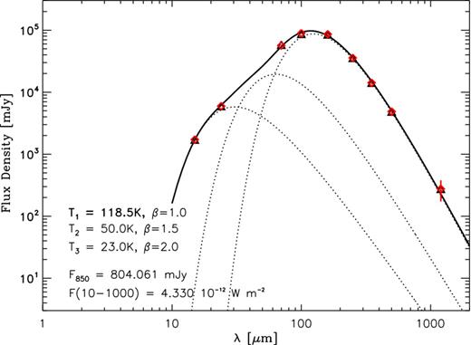
Observed integral SED of the Antennae, from ISOCAM 15 μm, Spitzer-MIPS 24 μm, Herschel-PACS 70, 100 and 160 μm, Herschel-SPIRE 250, 350 and 500 μm and IRAM-MAMBO 1200 μm photometry. Black triangles are the flux values originating from the standard calibration of the respective instrument. Red diamonds are colour-corrected fluxes (colour correction only applied for the PACS and SPIRE photometry) according to the thermal components (dotted lines) fitted to result in a composite model SED (solid black line). Details of the modified blackbody fits are given in the figure legend as well as the 850 μm flux prediction used for dust mass determination and the total 10–1000 μm flux.
Similar to the IRAS FIR flux definition (Lonsdale & Helou 1985; Helou et al. 1988) and its extension to the 170 μm ISOPHOT filter (Stickel et al. 2000), we use a PACS FIR flux parameter for the wavelength range 59 to 206 μm (effective band width of the three PACS bands together), which is valid for the temperature range 20–80 K and emissivity indices n = 0–2, being the ranges of interest for galaxies. The conversion formula for the calculation of the PACS FIR flux parameter from the PACS 70, 100 and 160 μm monochromatic flux densities will be presented in detail in Klaas et al. (in preparation). The total FIR luminosity is derived from this FIR flux parameter in analogy to the IRAS FIR luminosity calculation in Sanders & Mirabel (1996). This is the input for the calculation of observational IR SFRs according to formula (3) in Kennicutt (1998).
STAR FORMATION IN THE ANTENNAE SIMULATIONS
Global star formation properties
The top three panels of Fig. 2 show colour-coded maps of the total gas surface densities, Σgas, indicating differences in the central morphologies obtained for three Antennae simulations providing a varying degree of pressure support in the star-forming gas by adopting three different EoS parameters (see Section 2), qEoS = 1.0, qEoS = 0.1 and qEoS = 0.01 (from left to right). Each gas surface density map is overlaid with contours of the SFR surface density ΣSFR. For all three parameters, we find a similar large-scale morphology: the nuclei of the progenitor discs are still well separated, but connected by a ridge of high-density gas. In the case of very efficient feedback (qEoS = 1.0; K10-Q1.0), a high-density overlap region forms, but the highest densities are found in the galactic nuclei. In the simulations K10-Q0.1 and K10-Q0.01 with less vigorous feedback (qEoS = 0.1 and qEoS = 0.01), the high surface density regions tend to become tighter and more pronounced in the overlap (middle and right top panels). As a consequence we also find an increasing number of low-density (‘void’) regions inside the discs for lower values of qEoS ≤ 0.1 due to the decreasing pressure support in the star-forming gas. The star formation contours directly support this picture. Lowering the effective pressure, and hence the stellar feedback, in star-forming regions leads to more confined, localized regions of intense star formation activity. In the bottom panels of Fig. 2, we show the corresponding contours of the gas surface density and overplot all stellar particles (with individual masses of mstar = 6.9 × 10⁴M⊙), colour-coded according to their ages, having formed in the last τ < 15 Myr (blue), 15 Myr < τ < 50 Myr (green) and 50 Myr < τ < 100 Myr (red).4 This period corresponds to the time-span of the interaction-induced rise in the star formation activity during the recent second encounter. The youngest stars (blue) form predominantly in regions of currently high gas densities, i.e. in the centres, the overlap region, and in the arc-like features along the discs, very similar to observations of the youngest clusters in the Antennae (Whitmore et al. 1999, 2010; Wang et al. 2004b). This qualitatively confirms our earlier results in Karl et al. (2010), indicating that our conclusions are robust to altering the parameters of the adopted star formation feedback algorithm. However, Fig. 2 also shows that the star formation in the galaxy centres is much more pronounced in run K10-Q1.0 with qEoS = 1.0 (bottom left panel), while the overlap starburst gains more relative importance for runs K10-Q0.1 (qEoS = 0.1) and K10-Q0.01 (qEoS = 0.01; see also below). Furthermore, young stars (τ < 50 Myr) tend to be more concentrated in the overlap region and the well-defined arcs in the remnant spirals, while older stars (50 Myr < τ < 100 Myr) are dispersed more evenly throughout the discs. This captures a similar trend observed in the Antennae (e.g. Zhang et al. 2001, their fig. 2). Therefore we conclude that, within a range of feedback efficiencies qEoS ≲ 0.1, the overlap starburst seems to be driven by the most recent episode of star formation in the Antennae, which was induced by the second close encounter, while for values approaching the full stellar feedback (qEoS ≳ 0.5) the overlap starburst is significantly suppressed.
![Projected gas surface density and star formation in the central ±18 kpc of the galactic discs for the three Antennae simulations (K10-Q1, K10-Q0.1 and K10-Q0.01) with different values for the parameter for the softened EoS, qEoS = 1.0 (left), qEoS = 0.1 (middle) and qEoS = 0.01 (right). Top panels: projected gas surface density overlaid with contours of the SFR surface density. The contours correspond to levels of $\log (\Sigma _{\rm SFR}\,/[{\, {\rm M}_{{\odot }}}\,{\rm yr}^{-1} \,{\rm kpc}^{-2}]) = -6,\, -5, \ldots , \,-3,\, -2$, respectively. Bottom panels: gas surface density contours and stellar particles formed within the last 100 Myr, colour-coded by their age (see legend).](https://oup.silverchair-cdn.com/oup/backfile/Content_public/Journal/mnras/434/1/10.1093_mnras_stt1063/1/m_stt1063fig2.jpeg?Expires=1716393485&Signature=SsEMkk9T8X5lrPnkcT6H-7aTAVoN9BrbWQoOXFVVlrpm-LDxxCuBFJps-4uei-wvE~n13KWFPFpabgPvPN4XU65PFSa3zjUNr3qYeVLduaTkzYGw6aB79XlJl6XWU706M2HgEJPa7jq-9v93VTMXndT5ZWnTDejmFcVmy-IbpsEBcOaQq4JgF6AeNbwow1shtO8tYwUZSbLMUSlIvSGBBsJQatr-Il-Lf4y232sg9RuNF1zByLYvS4UgLHZLrQPNroH~gEw-DdxNeOQDe-A02XkpueAEIKaNxWt7TfvJBSUrzKCUq4GbW80H8fqoBP~xj7fbRDlCyplt7DknaRgTyg__&Key-Pair-Id=APKAIE5G5CRDK6RD3PGA)
Projected gas surface density and star formation in the central ±18 kpc of the galactic discs for the three Antennae simulations (K10-Q1, K10-Q0.1 and K10-Q0.01) with different values for the parameter for the softened EoS, qEoS = 1.0 (left), qEoS = 0.1 (middle) and qEoS = 0.01 (right). Top panels: projected gas surface density overlaid with contours of the SFR surface density. The contours correspond to levels of |$\log (\Sigma _{\rm SFR}\,/[{\, {\rm M}_{{\odot }}}\,{\rm yr}^{-1} \,{\rm kpc}^{-2}]) = -6,\, -5, \ldots , \,-3,\, -2$|, respectively. Bottom panels: gas surface density contours and stellar particles formed within the last 100 Myr, colour-coded by their age (see legend).
Thanks to the very good spatial resolution of the Herschel-PACS instrument in the FIR, the previously determined IR SEDs of individual star-forming knots (see e.g. Brandl et al. 2009) could be augmented by additional flux estimates at 70 μm, 100 μm and 160 μm (Klaas et al. 2010; Klaas et al., in preparation). The improved analysis described in Section 2.3 allows for a precise determination of the total FIR luminosities and SFRs in individual knots yielding integrated SFRs of |${\rm SFR}^{\rm 4038} = (1.57 \pm 0.04) {\, {\rm M}_{{\odot }}}\,{\rm yr}^{-1}$| and |${\rm SFR}^{\rm 4039} = (0.72 \pm 0.02) {\, {\rm M}_{{\odot }}}\,{\rm yr}^{-1}$| in the nuclei of NGC 4038 and NGC 4039, and |${\rm SFR}^{\rm OvL} \gtrsim 6.93 {\, {\rm M}_{{\odot }}}\,{\rm yr}^{-1}$|, when taking the sum over all knots in the overlap region as a lower limit (i.e. knots ‘K1’ to ‘K4’; see fig. 3 in Klaas et al. 2010 for a definition). We compare these estimates to our simulated SFRs in the galactic nuclei of NGC 4038 and NGC 4039 (defined as the central region of each nucleus with a radius of 1 kpc), and the overlap region (chosen according to the central morphology of the simulations). Details are provided in Table 3, where we compare the total SFRs, the gas mass, the stellar mass formed in the last 15 Myr, and the FIR fluxes in the three PACS bands at 70 μm, 100 μm and 160 μm for the different specific regions in each simulation. In the case of efficient feedback (qEoS = 1.0 and qEoS = 0.5), the simulations show stronger star formation activity in the two nuclei compared to the overlap region. The simulations with low stellar feedback (qEoS = 0.1 and qEoS = 0.01) develop a very vigorous overlap starburst with SFRs of |${\sim }26 {\, {\rm M}_{{\odot }}}\,{\rm yr}^{-1}$| and |${\sim } 11 {\, {\rm M}_{{\odot }}}\,{\rm yr}^{-1}$|, which is higher than the observed lower limit of |${\gtrsim } 6.93 {\, {\rm M}_{{\odot }}}\,{\rm yr}^{-1}$| (by a factor of ∼1.5–4) together with a very low ratio of SFRnuclei/SFRoverlap = 0.11 and 0.09 compared to ≲0.33 in the Herschel-PACS observations. Simulation K10-Q0 without stellar feedback has the lowest gas masses and local SFRs of all simulations due to a very efficient star formation and gas consumption earlier in the simulation (see below). The total instantaneous SFRs in the five simulations show a large scatter within |$5.4 {\, {\rm M}_{{\odot }}}\,{\rm yr}^{-1}\lesssim {\rm SFR} \lesssim 30 {\, {\rm M}_{{\odot }}}\,{\rm yr}^{-1}$|, as measured from the simulated SPH particles at the time of best match (see Table 4). These values are in broad quantitative agreement with the range of observed values between ∼5 and 20 |${{\rm M}_{{\odot }}}\,{\rm yr}^{-1}$| (e.g. Zhang et al. 2001) and with the value of |${\rm SFR} = (19.1 \pm 1.4) {\, {\rm M}_{{\odot }}}\,{\rm yr}^{-1}$| we derive from the total IR luminosity in this paper (see Table 4). Therefore, without attempting a fine-tuned match, we conclude that adopting a rather inefficient parametrization for the thermal stellar feedback, such as in simulations K10-Q0.1 and K10-Q0.01, tends to give the most consistent results with the observed spatial distribution of star-forming regions in the Antennae system.
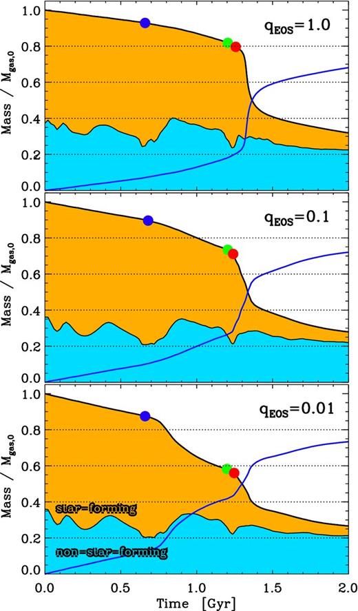
Time evolution of the mass in gas (upper black solid line) and newly formed stars (blue line) normalized to the initial gas mass in three Antennae simulations with different parameters for the softened EoS. Top panel: full feedback simulation K10-Q1 with qEoS = 1.0; middle panel: intermediate feedback simulation K10-Q0.1 with qEoS = 0.1; and bottom panel: the K10-Q0.01 simulation with very weak feedback, qEoS = 0.01. In addition, we distinguish between the dense star-forming gas (n > ncrit ≡ 0.128 cm−3) treated by the effective multi-phase model (orange) and non-star-forming gas (blue). The blue, green and red dots indicate the times of first pericentre, second pericentre and the time of best match in each simulation.
Local SFRs, gas masses, stellar mass formed within the last 15 Myr and FIR fluxes in the galactic nuclei and the overlap region for the five Antennae simulations (K10-Q1, K10-Q0.5, K10-Q0.1, K10-Q0.01 and K10-Q0) with qEoS = 1.0, qEoS = 0.5, qEoS = 0.1, qEoS = 0.01 and qEoS = 0.0.
| Simulation | Region | SFR (|${\, {\rm M}_{{\odot }}}\,{\rm yr}^{-1}$|) | Mgas (|$\times 10^{9} {\, {\rm M}_{{\odot }}}$|) | M⋆( < 15 Myr) (|$\times 10^7 {\, {\rm M}_{{\odot }}}$|) | f70/f100/f160 ( Jy)a |
|---|---|---|---|---|---|
| Nuc4038 | 1.71 | 1.60 | 2.30 | 4.59/6.54/4.12 | |
| qEoS = 1.0 | Nuc4039 | 4.08 | 1.68 | 6.30 | 12.6/17.1/8.01 |
| Overlap | 0.49 | 2.58 | 1.03 | 2.61/5.15/7.98 | |
| Nuc4038 | 4.55 | 1.49 | 6.98 | 10.3/14.3/6.63 | |
| qEoS = 0.5 | Nuc4039 | 2.85 | 1.15 | 4.72 | 10.4/12.7/5.74 |
| Overlap | 0.76 | 3.05 | 1.58 | 5.31/8.32/11.4 | |
| Nuc4038 | 0.92 | 0.58 | 1.48 | 4.48/5.24/2.81 | |
| qEoS = 0.1 | Nuc4039 | 2.02 | 0.10 | 3.39 | 9.91/11.8/5.65 |
| Overlap | 26.09 | 3.67 | 16.23 | 22.5/39.4/35.3 | |
| Nuc4038 | 0.49 | 0.26 | 0.75 | 3.03/3.29/1.53 | |
| qEoS = 0.01 | Nuc4039 | 0.44 | 0.14 | 0.55 | 3.67/3.76/1.59 |
| Overlap | 10.88 | 3.09 | 10.22 | 29.7/39.3/27.6 | |
| Nuc4038 | 0.99 | 0.13 | 1.48 | 4.16/3.92/1.47 | |
| qEoS = 0.0 | Nuc4039 | 0.46 | 0.15 | 0.70 | 3.31/3.44/1.35 |
| Overlap | 2.24 | 2.52 | 3.04 | 8.44/11.4/10.1 | |
| Nuc4038 | 1.57 ± 0.04 | 3.65 | − | 3.91 ± 0.12/6.73 ± 0.20/8.94 ± 0.45 | |
| Observationsb | Nuc4039 | 0.72 ± 0.02 | 1.34 | − | 1.91 ± 0.06/3.53 ± 0.11/3.40 ± 0.17 |
| Overlap | 6.93 ± 0.27 | 6.16 | − | 21.6 ± 0.4/31.4 ± 0.7/30.1 ± 1.1 |
a Fluxes at 70 μm, 100 μm and 160 μm, given in Jy, for models with gas-to-dust ratio 62:1 and the observations (see Section 2.3).
b SFRs are calculated from the total infrared luminosity, L(50-1000) μm, according to Kennicutt (1998), equation (3). FIR flux densities, gas masses and SFRs for the overlap region are estimated as a lower limit by summing up the emission from knots K1 − K4 (for D = 30.8 Mpc). See Klaas et al. (2010) for a definition of the different FIR knots. Observed gas masses denote molecular gas masses from Wilson et al. (2000) (see Klaas et al. 2010, table 2).
Reproducing the overlap starburst
In a first attempt to explain the large scatter in the star formation properties, we show the evolution of the gas masses for three simulations employing different parameters for the stellar feedback model in Fig. 3. The gas is separated into non-star-forming (blue) and star-forming gas phases (orange) based on the density criterion n > ncrit = 0.128 cm−3. All three simulations show a steady decrease in their gas mass (upper solid line) due to consumption by star formation from the very start of the simulations, corresponding to a gradual build-up of the new stellar component (blue solid line). However, due to the lower pressure support in the effective multi-phase model in the K10-Q0.01 simulation (bottom panel), a fraction of 12.5 per cent of the initial gas mass has already been turned into stars by the time of the first pericentre (blue dots), whereas the K10-Q1.0 simulation, with a more efficient stellar feedback (top panel), has only consumed about 7.2 per cent at the same time. The K10-Q0.1 case is intermediate with 10.4 per cent. The total fraction of non-star-forming gas (blue) stays constant to within ∼10 per cent around a level of 0.3 during the whole course of the simulated time-span (t < 2.0 Gyr), save some little ‘dips’ during episodes of induced star formation associated with the first and the second pericentre passages indicated by the blue (t = 0.66–0.68 Gyr) and green (t ≈ 1.20 Gyr) dots in Fig. 3. The more dramatic evolution can be seen in the star-forming gas (orange, n > ncrit = 0.128 cm−3) which gets efficiently depleted after the first pericentre in the K10-Q0.01 simulation with weak feedback (bottom panel), having consumed more than 41 per cent of the initial gas mass in the form of star-forming gas at the time of second pericentre. In contrast, in the full-feedback run (K10-Q1.0) there is still about 81 per cent of the initial gas mass remaining after the second encounter, which leads to a very rapid consumption of 40 per cent of the gas within the first ∼250 Myr after the final merger (red dots). The key difference is that the low feedback simulation consumes the nuclear gas reservoir before the best match in contrast with the full feedback simulation. In Table 3 we find that, with decreasing qEoS, the nuclear gas masses go down drastically – from nuclear gas masses of |$M_{\rm gas} = 1.6 \times 10^9 {\, {\rm M}_{{\odot }}}$| for qEoS = 1.0 to a factor of ∼10 lower in the other two runs. The gas masses in the overlap regions, on the other hand, show a less pronounced dependence on the chosen effective stellar feedback parameter, staying constant to within ∼40 per cent, while the SFRs increase significantly for the two lower-feedback simulations as discussed above.
A complementary view of this picture is offered by the star formation histories in the Antennae simulations (Fig. 4). The isothermal and quasi-isothermal simulations (K10-Q0 and K10-Q0.01) show quite similar initial SFRs of |${\sim } 3.6 {\, {\rm M}_{{\odot }}}\,{\rm yr}^{-1}$| and |${\sim } 3.2 {\, {\rm M}_{{\odot }}}\,{\rm yr}^{-1}$|. The SFRs for the simulations with efficient feedback and qEoS ≥ 0.5 (K10-Q0.5 and K10-Q1.0) are smaller by a factor of about ∼1.5 from the very start, while run K10-Q0.1 is intermediate with |${\rm SFR}(t = 0) \sim 2.6 {\, {\rm M}_{{\odot }}}\,{\rm yr}^{-1}$|. After the first pericentre (black arrow) runs K10-Q0 and K10-Q0.01 both experience a significant rise in their SFRs by more than a factor of 5, while the other three simulations show a more gradual increase. The low-feedback simulations show high total SFRs of |${\sim }30 {\, {\rm M}_{{\odot }}}\,{\rm yr}^{-1}$| (K10-Q0.1) and |${\sim }14 {\, {\rm M}_{{\odot }}}\,{\rm yr}^{-1}$| (K10-Q0.01) at the time of best match (see Table 4), powered by the short-lived overlap starburst shortly after the second pericentre. The full-feedback (K10-Q1.0) and intermediate-feedback (K10-Q0.5) simulations, on the other hand, build up very powerful nuclear starbursts after the final merger with a maximum total SFR of SFR|$_{\rm max}\sim 140 {\, {\rm M}_{{\odot }}}\,{\rm yr}^{-1}$| and SFRs at the best match of only |${\sim }7 {\, {\rm M}_{{\odot }}}\,{\rm yr}^{-1}$| and |${\sim }9 {\, {\rm M}_{{\odot }}}\,{\rm yr}^{-1}$| (Table 4), respectively. An equally powerful starburst is missing in the case of weaker stellar feedback with SFR|$_{\rm max} = 68.4 {\, {\rm M}_{{\odot }}}\,{\rm yr}^{-1}$| for the K10-Q0.1, and SFR|$_{\rm max} = 40.8 {\, {\rm M}_{{\odot }}}\,{\rm yr}^{-1}$| for the K10-Q0.01 simulations. Having consumed about half of its gas before the second pericentre, simulation K10-Q0 has the lowest SFR of all simulations during the time between second pericentre and final merger with a |${\rm SFR} \sim 5.4 {\, {\rm M}_{{\odot }}}\,{\rm yr}^{-1}$| at the best match. Leaving aside simulation K10-Q0 without stellar feedback, we find a clear anti-correlation between the height of the maximum SFRs after the first and second pericentres in the sense that simulations having higher star formation peaks after the first pericentre have correspondingly lower star formation peaks after final coalescence and vice versa. Note also that this trend, interestingly, yields very similar gas fractions in these simulations after final coalescence of the galaxies (see Fig. 3), differing by less than ∼5 per cent at 2 Gyr. It is, however, not directly reflected in the SFRs at the time of best match, which we find shortly (∼30–50 Myr) after the second encounter but before the time of maximum star formation activity (see Fig. 4). This is first due to a more rapid gas consumption during the first pericentre in the weaker feedback runs and secondly due to a weaker pressure support in the star-forming gas phase in the K10-Q0.1 and K10-Q0.01 simulations making the gas in the overlap region more susceptible to local shock-induced fragmentation and subsequent star formation, as discussed above.
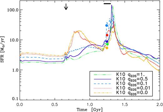
Star formation histories for the five Antennae simulations with varying feedback parameters: qEoS = 1.0 (green), qEoS = 0.5 (purple), qEoS = 0.1 (blue), qEoS = 0.01 (red) and qEoS = 0.0 (orange). The arrow gives the time of first close encounter, while the bar indicates the time between second close encounter and final merger. The time of best match is denoted by the coloured dots for each simulation.
Global SFRs, gas masses and FIR fluxes, measured over the entire system, for all Antennae simulations (K10-Q1, K10-Q0.5, K10-Q0.1, K10-Q0.01 and K10-Q0) with varying feedback parameters: qEoS = 1.0, qEoS = 0.5, qEoS = 0.1, qEoS = 0.01 and qEoS = 0.0.
| Simulation | SFRa | Mgas | ftot, 70/ftot, 100/ftot, 160b |
|---|---|---|---|
| qEoS = 1.0 | 7.16 | 13.2 | 31.0/49.6/46.8 |
| qEoS = 0.5 | 8.74 | 12.2 | 34.0/51.7/45.1 |
| qEoS = 0.1 | 30.1 | 11.8 | 48.5/76.8/66.4 |
| qEoS = 0.01 | 14.3 | 9.28 | 49.2/65.1/46.7 |
| qEoS = 0.0 | 5.36 | 8.38 | 26.8/34.0/26.7 |
| Observationsc | 19.1 ± 1.4 | ∼9.6 | 56.5/89.4/86.1 |
aUnits for the numbers given in Columns 2–4 are in [|${\, {\rm M}_{{\odot }}}\,{\rm yr}^{-1}$|], [|$\times 10^{9} {\, {\rm M}_{{\odot }}}$|] and [ Jy], respectively.
bTotal fluxes at 70 μm, 100 μm and 160 μm, given in Jy, for models with gas-to-dust ratio 62:1.
c For the observed SFRs and FIR fluxes we give values re-analysed for this paper (see Section 2.3, Klaas et al., in preparation). Total gas masses in the galactic discs for H2 and H i are adopted from Gao et al. (2001) and Hibbard et al. (2001), assuming a distance of D = 30.8 Mpc and a CO-to-H2 conversion factor |$\alpha _{\rm CO} = 0.8 {\, {\rm M}_{{\odot }}}\,{\rm pc}^{-2}\, (K {\rm km\, s}^{-1})^{-1}$| (Downes & Solomon 1998).
Overall, the star formation histories are complex and there is a large scatter in the SFRs at the time of best match (being defined as the time when simulated and observed morphology and line-of-sight kinematics are most similar), depending on the parameter choice of qEoS for the stellar feedback model. This, e.g., leads to very similar SFRs at the time of best match in the full-feedback simulation K10-Q1, employing a vigorous feedback, and the isothermal simulation K10-Q0 with no feedback at all. Therefore, global properties like the total SFRs and the total gas masses alone seem to be a degenerate diagnostic when comparing to observations.
Comparison with observed CO maps
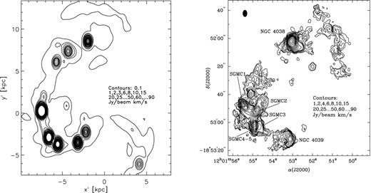
Left-hand panel: synthetic CO map of the central regions of the Antennae from the K10-Q0.01 simulation. The integrated CO masses are obtained in a two-step process. First, the H2 surface densities are obtained from the SFR surface densities of the SPH particles using an ‘inverse’ Bigiel et al. (2008) relation. Then, adopting a conversion motivated by the observations (Wilson et al. 2000), we map H2 masses back to CO integrated intensities (see text for details). Right-hand panel: CO(1–0) integrated intensity map, adapted from fig. 1 in Wilson et al. (2000). The two galactic nuclei and five supergiant molecular clouds in the overlap region are indicated. The filled black oval in the top left corner gives the size of the synthesized beam (3.15 × 4.91 arcsec2) in the observations. Reproduced by permission of the AAS.
COMPARISON WITH FAR-INFRARED OBSERVATIONS
In Fig. 6 we compare Herschel-PACS data (top row; see Section 2.3) in three photometric wavebands centred on 70 μm, 100 μm and 160 μm with the simulated FIR RT maps of the K10-Q0.5, K10-Q0.1 and K10-Q0.01 simulations (bottom three rows; see Section 2.2). Being an a priori un-constrained parameter in the RT model (see Section 2.2), we tested for variations in the gas-to-dust ratio (not shown) but found only negligible changes in the FIR morphology for gas-to-dust ratios between 62:1 and 124:1 in all three FIR bands. Therefore, we only show the simulated maps adopting a gas-to-dust ratio of 62:1, which generally gives the best match to the observed SED in the Antennae (see below). We choose a lower cut in the surface brightness determined by the mean noise level corrected for correlated noise above the mean background in each band. The upper limits in the colour scheme are set by the maximum surface brightness levels of the observations.
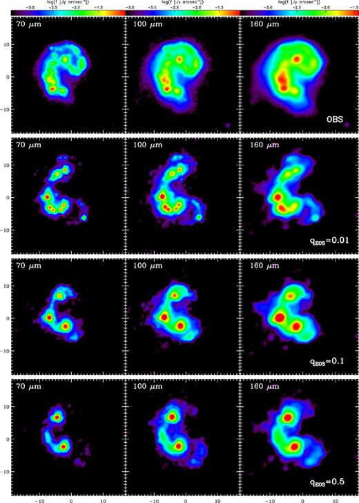
Synthetic 3D RT maps of the central regions of the Antennae at 70 μm (left-hand column), 100 μm (middle column) and 160 μm (right-hand column) for simulations K10-Q0.01, K10-Q0.1 and K10-Q0.5 with a gas-to-dust ratio 62:1 (bottom three rows). The simulated maps are compared to Herschel-PACS observations in the same bands (top row; see Section 2.3, Klaas et al. 2010, Klaas et al., in preparation). Surface brightness is given in logarithmic units of Jy arcsec−2.
Emission in the FIR bands reveals the sites of recent star formation that are still embedded in the dusty molecular clouds from which they have formed. The simulated FIR properties vary significantly depending on the adopted efficiency of the sub-grid stellar feedback model. Simulations K10-Q0.5 and K10-Q0.1 (two bottom rows) show only a small number of emission peaks, most dominant either in the two nuclei (K10-Q0.5) or in the overlap region (K10-Q0.1) in all three simulated bands. Simulation K10-Q0.01 (the second row of Fig. 6), on the other hand, shows a well-defined pattern of sequential, confined star-forming knots along the overlap region very similar to the observations (top row). However, there are also two additional star-forming knots near the northern nucleus which are not detected at a similar level in the observations. As seen in Tables 3 and 4, more than ≳ 50 per cent of the FIR emission in each band originates from the overlap region in simulations K10-Q0.01 and K10-Q0.1, compared to only 6–14 per cent (12–30 per cent) from the two nuclei in NGC 4038 and NGC 4039 combined in K10-Q0.01 (K10-Q0.1). A similar percentage (10–15 per cent) is observed in the combined fluxes of the two nuclei in all three Herschel-PACS bands. The combined emission from the observed knots in the overlap regions gives a lower bound for the total emission from the overlap region, yielding a total of ∼35–39 per cent for the three bands. We find a very good agreement between the observed FIR surface brightness maps and those of simulation K10-Q0.01.
Apart from differences in the spatial distribution of the simulated and observed FIR emission due to the specific adopted stellar feedback parameters, there are also some characteristic differences with respect to the observed FIR maps which are generic to all the simulations. These are mostly caused by slight differences in the underlying overall projected gas morphologies in the simulations, as discussed in Section 3 (see Fig. 2). Most notably, the simulated RT maps in the bottom three rows in Fig. 6 indicate some low-level emission from the southern disc (NGC 4039) which is not observed (top row). This makes the observed discs look slightly more tilted to the north-west than the simulated ones. Furthermore, the dominant emission peak is found in the northern part of the overlap region in the simulations which is slightly at odds with the highest emission being observed in knots K1 and K2, at the southern end of the overlap region in the Antennae (fig. 3 in Klaas et al. 2010). Comparing the global distribution of FIR emission, we do not find equally strong spatially extended emission in the simulated progenitor discs. This may be best seen in the northern spiral, e.g. comparing the arc-like feature which is clearly detected in the 100 μm and 160 μm Herschel maps (top middle and left panel) to the very localized emission in the simulations in these bands (bottom three middle and left panels). This may partly be caused by different large-scale gas morphologies, as discussed above, and, to some extent, by resolution effects and/or restrictions in the adopted sub-grid model for the stellar feedback, leading to a spatially confined star formation in high-density regions, which in turn is seen in the simulated FIR maps.
To highlight the striking differences in the simulated FIR properties when adopting different feedback parameters we present in Fig. 7 the two most extreme cases from our sample, the full-feedback simulation K10-Q1 with qEoS = 1 and the isothermal simulation K10-Q0 without any stellar feedback, i.e. qEoS = 0, both with a gas-to-dust ratio of 62:1. In the K10-Q1 simulation, emission from the overlap region is feeble, especially at the shorter wavelengths, which reveals a prevalence of cold dust in this region. The observed overlap starburst is missing entirely in the synthetic FIR maps. In simulation K10-Q0 a large number of spatially confined peaks of emission develops in the three FIR bands and the emission shows a secondary peak at the southern end of the overlap region. Due to the high prior gas consumption and a resulting low SFR of |${\sim }5.4 {\, {\rm M}_{{\odot }}}\,{\rm yr}^{-1}$| at the time of best match, however, the surface brightness is much lower compared to the best-matching simulation K10-Q0.01 (as discussed in Section 3).
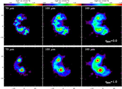
Synthetic 3D RT maps of the central regions of the Antennae at 70 μm (left-hand column), 100 μm (middle column) and 160 μm (right-hand column) with a gas-to-dust ratio 62:1, highlighting the large scatter in FIR properties when adopting the two extreme parameter choices for the stellar feedback model in our sample: the simulation without stellar feedback K10-Q0 with qEoS = 0.0 (top) and the full-feedback simulation K10-Q1.0 with qEoS = 1.0 (bottom). Surface brightnesses are given in logarithmic units of Jy arcsec−2.
Fig. 8 shows the simulated SEDs of the three Antennae simulations with qEoS = [1.0, 0.1, 0.01] in comparison to observations of the FIR fluxes in the Antennae at 70 μm, 100 μm and 160 μm, given as the filled dots with error bars, and a model of three combined modified blackbody spectra fitted to IR data points within 10-1000 μm, given as the thin black line (see Fig. 1 and Section 2.3). The different lines for each simulation probe varying gas-to-dust models with a standard Milky Way value of 124:1 (dotted lines) and lower values employing successively more dust with ratios of 83:1 (dashed lines) and 62:1 (solid lines). Increasing the total amount of dust in the RT simulations leads to increasingly lower dust temperatures seen as shifts in the peak emission towards longer wavelengths. The observed spectral shape is best reproduced with a low gas-to-dust ratio of 62:1 (solid lines). In particular, this choice leads to a steep slope between 70 μm and 100 μm, similar to the observed data points, with a ratio f100 μm/f70 μm = 89.4/56.5 ≈ 1.6, as well as the flat and subsequently declining part near the peak of the spectrum between 100 μm and 160 μm. Only for wavelengths below ≲ 60 μm the simulated SEDs seem to drop a bit too fast compared to the fitted modified blackbody spectra. This is in part due to the fact that, at these and shorter wavelengths we start to miss some significant contributions to the total flux density from stochastically heated small dust grains, or, in the mid-infrared, from polycyclic aromatic hydrocarbons (PAHs).
![Comparison of the total SED of RT calculations for the three different Antennae simulations K10-Q1, K10-Q0.1 and K10-Q0.01 with observations. Dotted lines correspond to SEDs calculated assuming a standard Milky Way gas-to-dust ratio of 124:1, while for the dashed and solid lines the ratio is reduced to a factor of 83:1 and 62:1, respectively. The small circles give the total fluxes obtained with Herschel-PACS observations at 70 μm, 100 μm and 160 μm (see Fig. 1 and Section 2.3, Klaas et al. 2010; Klaas et al., in preparation). The total (intrinsic+systematic) photometric error is given as bars, where we estimated the intrinsic photometric error as ∼[50, 50, 90] mJy and the systemic error as ∼[3 per cent, 3 per cent, 5 per cent] at 70 μm, 100 μm and 160 μm, respectively. The thin black line gives a theoretical fit to the observed IR SED using a three-component modified blackbody model (see Section 2.3).](https://oup.silverchair-cdn.com/oup/backfile/Content_public/Journal/mnras/434/1/10.1093_mnras_stt1063/1/m_stt1063fig8.jpeg?Expires=1716393485&Signature=bbUzapl5JoFX6EMoOD8bujarpdxJtprz7VtdSWsddODx0FRnn56J2dCq7hhs5QRrbSJJ-YniQYAS4GFF8xwbUK6hpHaeb7zWHyj4HBJQR~nIK9c7nbvMTuZVjDzo~drX7uL0-W9ixJGXjMF4sDMPnqebWV9lBLQi3mhSICaAeHVM-P6Bw6qeptD91Eg3HD2YLQwkNkUSRVYNfax2T6-AZroE96Jyaa-~j2juhHXkAXBbTh7KuRIbhC8esfoimvg5ezt64pDu245UttWZmgI0PqBLU4x~EV7Wq8ZBHOOLQ5aZyUF9~ZqPBPrvi2YqcCeA4wxloxT1Ar933KOi2NyE1w__&Key-Pair-Id=APKAIE5G5CRDK6RD3PGA)
Comparison of the total SED of RT calculations for the three different Antennae simulations K10-Q1, K10-Q0.1 and K10-Q0.01 with observations. Dotted lines correspond to SEDs calculated assuming a standard Milky Way gas-to-dust ratio of 124:1, while for the dashed and solid lines the ratio is reduced to a factor of 83:1 and 62:1, respectively. The small circles give the total fluxes obtained with Herschel-PACS observations at 70 μm, 100 μm and 160 μm (see Fig. 1 and Section 2.3, Klaas et al. 2010; Klaas et al., in preparation). The total (intrinsic+systematic) photometric error is given as bars, where we estimated the intrinsic photometric error as ∼[50, 50, 90] mJy and the systemic error as ∼[3 per cent, 3 per cent, 5 per cent] at 70 μm, 100 μm and 160 μm, respectively. The thin black line gives a theoretical fit to the observed IR SED using a three-component modified blackbody model (see Section 2.3).
More important for the SEDs of the simulated data, however, is the choice of the adopted stellar feedback parameter qEoS. While the adopted gas-to-dust ratio changes mostly the spectral shape, the parameter for the stellar feedback changes significantly both the spectral shape and the total flux of the simulated SEDs due to differences in geometry, total gas mass and SFRs between the simulations. Simulation K10-Q0.01 has the smallest amount of gas (and dust) in the actively star-forming regions (see Table 3) combined with a relatively high SFR at the time of best match, yielding a strong emission from hot dust at shorter wavelengths. Simulations K10-Q0.1 and K10-Q1.0, however, show a spectral shape peaking at longer wavelengths due to their larger reservoirs of gas (and dust).6 The best agreement to the observed data points both in terms of the total flux level and the spectral shape is reached for simulation K10-Q0.1 (i.e. with a low feedback efficiency of qEoS = 0.1) and a gas-to-dust ratio of 62:1 (red solid line in Fig. 8). The SEDs of simulations K10-Q0.01 and K10-Q0.1 peak at a value of ∼65 Jy at 99 μm and ∼81 Jy at 116 μm (compare also with Fig. 6), respectively, similar to the peak value of 97.4 Jy at 118 μm in the modified blackbody spectrum (thin black line).
SUMMARY AND DISCUSSION
In this paper, we analyse the global and spatially resolved star formation properties in a suite of hydro-dynamical simulations of the Antennae galaxies in order to understand the origin of the observed central overlap starburst. Our aim is to assess the impact of variations in the applied thermal stellar feedback on observable simulated star formation properties at the time of best match, in the spirit of a study on the Mice galaxies by Barnes (2004) who investigated variations due to the applied star formation law. Using a state-of-the-art dust RT code (Lunttila & Juvela 2012, see Section 2.2) we directly compare synthetic FIR maps and SEDs with re-analysed Herschel-PACS observations (Klaas et al. 2010, see Section 2.3; Klaas et al., in preparation). This is the first time that the FIR properties of a specific local merger system are compared in quantitative detail to the simulated FIR properties of a dynamical merger model.
The distributed extra-nuclear starburst in the Antennae galaxies is plausibly a natural consequence of induced star formation in high-density regions in the overlapping galactic discs after the recent second close encounter. This is the only phase in the simulations when a gas-rich, star-bursting overlap region forms and when we find spatially confined areas of high star formation activity and of similar extent as observed in the overlap region in the Antennae (e.g. Mirabel et al. 1998; Wilson et al. 2000; Zhang et al. 2001; Wang et al. 2004b; Zhang et al. 2010). We confirm that this result holds for a range of adopted stellar feedback efficiencies of the sub-grid star formation model (see e.g. Fig. 2). However, we find a trend that the overlap star formation activity is significantly suppressed for values approaching the full stellar feedback simulation (qEoS ≲ 1; Springel & Hernquist 2003). Best qualitative agreement with observations is obtained using a rather inefficient parametrization, 0.01 ≲ qEoS ≲ 0.1, for the thermal stellar feedback. This is in agreement with recent results by Hopkins & Quataert (2010) who advocated a range of qEoS = [0.125, 0.3] by comparing model predictions and simulations for different values of qEoS to the gas properties in observed star-forming systems.
The star formation histories in the different simulations are complex and there is a large scatter in the global observable properties, e.g. the total gas mass, SFR and FIR fluxes, at the time of best match (see Table 4; Figs 3 and 4), even though they only differ in the chosen parameter for the thermal stellar feedback. We find that additional information provided by a spatially resolved analysis of these properties is needed to break degeneracies in the model assumptions.
Synthetic FIR maps at 70 μm, 100 μm and 160 μm (Figs 6 and 7) show very different FIR surface brightness properties for varying efficiencies of the thermal stellar feedback. We find that, for a rather inefficient stellar feedback formalism with 0.01 ≲ qEoS ≲ 0.1, the simulated maps are in good agreement with the spatially resolved FIR observations. This quantitatively supports results from a simple conversion of the simulated local star formation to molecular hydrogen surface densities that compares well with the observed integrated CO intensity map (Fig. 5). We propose that the reason for this is that the simulations employing low feedback efficiencies encompass a sweet spot between a moderate previous gas consumption history together with a higher susceptibility to induced star formation after the second close encounter caused by the weak thermal support against local gas collapse.
Probing synthetic SEDs in the FIR using different gas-to-dust ratios, we find that a low gas-to-dust ratio of 62:1 yields spectral shapes of the simulated SEDs that are in good agreement with a simple modified blackbody spectrum fitted to the observed data points, however with significantly lower flux densities in the simulated SEDs (Fig. 8). For simulations K10-Q1.0, K10-Q0.1 and K10-Q0.01 with gas-to-dust ratios of 62:1, the average flux decrements are 43.9 per cent, 18.6 per cent and 31.7 per cent within 50–280 μm. The synthetic FIR SED of the best-fitting simulation, K10-Q0.1 (i.e. with qEoS = 0.1), peaks at a value of ∼81 Jy at 116 μm, similar to the peak value of 97.4 Jy of the fitted modified blackbody spectrum at 118 μm. A comparison with the observed L250–SFR relation (Hardcastle et al. 2013, cf. formulae on page 13; their fig. 9) reveals that the SFRs estimated from our modelled flux densities at 250 μm seem to be systematically lower (by an average of 0.4 dex) than the SFRs in the hydrodynamic simulations. About half of the simulations lie within the observed uncertainty in the SFRs, which is given as ±0.5 dex (Hardcastle et al. 2013, their fig. 9). Again, we find that the agreement is best for simulations with low gas-to-dust ratios of 62:1.
Is the seemingly favoured low gas-to-dust ratio of 62:1 realistic? Assuming all the metals to be locked up in the dust grains and none left in the gas phase, this value corresponds to a lower limit in the metallicity being slightly sub-solar (Z ∼ 0.8 Z⊙). This is well within estimates for individual young star clusters in the Antennae having metallicities of roughly solar (0.5 < Z/Z⊙ < 1.5, see fig. 11 in Bastian et al. 2009). Metal abundances determined in the hot ISM phase are found to vary widely from sub-solar (∼0.2 Z⊙) to highly super-solar ∼20 Z⊙ (Fabbiano et al. 2004; Baldi et al. 2006a). So a lower metallicity limit of Z ≥ 0.8 Z⊙ is not ruled out by the observations.
On the other hand, we can try and estimate the observed gas-to-dust ratio. These estimates depend critically on the adopted CO-to-H2 conversion factor. If we identify the total gas mass in the discs as |$M_{\rm gas}^{\rm {disc}} \approx M_{\rm H\,\small {I}}^{\rm {disc}} + M_{{{\rm H}_2}}$| (|$M_{{{\rm H}_2}} = M_{{{\rm H}_2}}^{\rm {disc}}$|, since there is no H2 detected in the tidal arms), we obtain a gas-to-dust ratio of G/D ∼ 670 for |$\alpha _{\rm CO} = 4.78 {\, {\rm M}_{{\odot }}}\,{\rm pc}^{-2}\, (K {\rm km\, s}^{-1})^{-1}$| (Gao et al. 2001), and G/D ∼ 135 for |$\alpha _{\rm CO} = 0.8 {\, {\rm M}_{{\odot }}}\,{\rm pc}^{-2}\, (K\, \,{\rm km\, s}^{-1})^{-1}$| as frequently adopted in starbursts (Downes & Solomon 1998) and consistent with the latest analysis (Bolatto, Wolfire & Leroy 2013) and values obtained in the nucleus of NGC 4038 and the overlap regions in the Antennae (Zhu et al. 2003). Here we have used |$M_{{{\rm H}_2}} = \alpha _{\rm CO}\cdot L_{\rm CO}$| with LCO taken from Gao et al. (2001), |$M_{\rm H\,{\small I}}^{\rm {disc}}$| from Hibbard et al. (2001), and all quantities scaled to the same distance. While the uncertainty is large depending on our choice for αCO, these values seem to favour a higher gas-to-dust ratio than the one we have chosen to match the observed FIR SED.
What else could influence the simulated SED shape? Changes in the assumed distance used to match the observations would result only in changes of the normalization in the simulated fluxes, e.g. a distance change of ∼10 per cent changes the fluxes by ∼20 per cent. They would, however, have no influence on the SED shapes. Higher dust masses due to higher initial gas fractions or due to cooling and subsequent accretion from a hot galactic halo (Moster et al. 2011), however, might lead to redder simulated SEDs by increasing the total dust mass at any given time throughout the merger process, without invoking low gas-to-dust ratios. Accordingly, higher SFRs might counteract this trend, most likely, however, to a much smaller extent (see e.g. Hayward et al. 2011). We plan to test this hypothesis in future hydrodynamic simulations including the effects of metal evolution and the presence of galactic hot haloes.
The specific form of the stellar IMF also affects the simulated SEDs. The star formation and feedback model we use (Springel & Hernquist 2003) intrinsically assumes a Salpeter IMF, e.g. for computing the supernova rates and hence the feedback energy and gas return fractions to the surrounding ISM, producing only about half of the luminous stars with respect to a Chabrier (2003) IMF. For consistency, we also use a Salpeter IMF to compute the stellar emission in the RT calculations. Choosing a Chabrier IMF to test the impact of the IMF on the RT calculations, we found that a lower mass-to-light ratio (by ∼0.1–0.2 dex) in this case leads to an increase in the FIR emission by a similar amount (20–50 per cent). Furthermore, the higher relative fraction of massive young stars leads to higher dust temperatures, with the emission peaking at shorter wavelengths and shifting the SEDs towards the blue. As a result, an even lower gas-to-dust ratio would be required to match the observed SEDs in Fig. 8. Adopting a Chabrier IMF in the star formation and feedback model would probably yield a more vigorous stellar feedback due to the higher fraction in massive stars. The consequences of these changes, however, are less obvious, requiring further self-consistent simulations.
The RT calculation we use here assumes that the dust grains are in thermal equilibrium with the local radiation field. However, stochastic heating of very small dust grains by absorption of starlight results in high-temperature transients, during which the absorbed energy is re-radiated mainly at mid-infrared wavelengths. It has been shown that this mechanism may have a significant effect on the emission at 70 μm, depending on the local stellar radiation field (Silva et al. 1998; Li & Draine 2001). At the FIR wavelengths, which are the focus of this article, the emission from large grains at the equilibrium temperature, however, is expected to be dominant.
Another factor affecting the results from the RT simulations is the treatment of small-scale structure in the ISM. While we assume a smooth density distribution at the scale of individual cells (∼40 pc in the central parts of the galaxies), the ISM definitely shows structures on much smaller scales. We do not include any sub-scale modelling of photodissociation regions (PDRs) around young stars or clumpy molecular clouds. In the simulations discussed in this article the effect of PDRs is likely to be relatively small, because a large fraction of the total luminosity is from stars older than 10 Myr. On the other hand, the non-uniform dust density distribution is known to have a potentially significant effect on the dust temperature distribution and infra-red emission (e.g. Witt & Gordon 1996; Doty, Metzler & Palotti 2005; Schunck, Hegmann & Sedlmayr 2007). A proper treatment of the clumpy cloud structure using a sub-grid model is to be considered in future studies.
In this paper we have shown as a proof of principle that variations in parameters governing the stellar feedback model result in unambiguous changes in the observable FIR properties. Without attempting a fine-tuned match, in our adopted star formation and feedback model a rather inefficient thermal stellar feedback formulation (0.01 ≲ qEoS ≲ 0.1) seems to be clearly preferred both by simulated FIR maps and by SEDs, similar to the recently advocated range by Hopkins & Quataert (2010). Recently, more realistic numerical models also include metal evolution, kinetic and thermal stellar feedback (e.g. Hopkins, Quataert & Murray 2011), feedback from active galactic nuclei (e.g. Choi et al. 2012), effects from magnetic fields (Kotarba et al. 2010) and accretion from hot galactic gas haloes (Sinha & Holley-Bockelmann 2009; Moster et al. 2011). Tests with other codes, e.g. AMR grid codes, might also prove useful to single out numerical artefacts inherent to different methods using the same initial conditions (see e.g. Agertz et al. 2007, for a comparison between SPH- and grid-based hydrodynamical methods). The next step is to compare further mock observations of the simulation results to multi-wavelength observations of the Antennae. In this context, constraints from detailed X-ray maps are particularly important (Fabbiano, Zezas & Murray 2001; Fabbiano et al. 2004; Baldi et al. 2006a,b). In doing so, using the Antennae system as a ‘standard ruler’, we can further gauge the employed star formation algorithms and simultaneously possibly gain further insights into the physics of merger-induced star formation.
We thank the anonymous referee for useful suggestions and comments which improved the presentation of the paper. This work was supported by the Science & Technology Facilities Council [grant number ST/J001538/1]. PHJ acknowledges the support of the Research Funds of the University of Helsinki. TL and MJ acknowledge the support of the Academy of Finland through grants No. 132291 and No. 250741. Many thanks to Christine Wilson for useful discussions and the permission to reproduce fig. 1 from Wilson et al. (2000) in Fig. 5. PACS has been developed by a consortium of institutes led by MPE (Germany) and including UVIE (Austria); KUL, CSL, IMEC (Belgium); CEA, OAMP (France); MPIA (Germany); IFSI, OAP/AOT, OAA/CAISMI, LENS, SISSA (Italy); IAC (Spain). This development has been supported by the funding agencies BMVIT (Austria), ESA-PRODEX (Belgium), CEA/CNES (France), DLR (Germany), ASI (Italy) and CICYT/MCYT (Spain). The simulations in this paper were performed on the OPA cluster supported by the Rechenzentrum der Max-Planck-Gesellschaft in Garching.
Herschel is an ESA space observatory with science instruments provided by European-led Principal Investigator consortia and with important participation from NASA.
The corresponding stellar masses formed in the last τ < 15 Myr are given in Table 3 for different regions in the merger.
One should bear in mind, however, that these maps still fundamentally represent the simulated SFRs and no CO(1–0) emission, which we do not model in the simulations presented here, even if we will call the converted simulated SFR maps ‘CO-maps’ (instead of ‘SFR-to-CO-maps’) for simplicity for the rest of this paper.
Note here that average dust temperatures depend much more strongly on the total dust mass than on the SFR, or the bolometric luminosity Lbol, causing the SED to appear ‘warmer’ for smaller dust masses (e.g. Hayward et al. 2011).
