


Abstract
Many supernova remnants (SNRs) are characterized by a knotty ejecta structure. The Vela SNR is an excellent example of remnant in which detached clumps of ejecta are visible as X-ray emitting bullets that have been observed and studied in great detail. We aim at modelling the evolution of ejecta shrapnel in the Vela SNR, investigating the role of their initial parameters (position and density) and addressing the effects of thermal conduction and radiative losses. We performed a set of 2D hydrodynamic simulations describing the evolution of a density inhomogeneity in the ejecta profile. We explored different initial setups. We found that the final position of the shrapnel is very sensitive to its initial position within the ejecta, while the dependence on the initial density contrast is weaker. Our model also shows that moderately overdense knots can reproduce the detached features observed in the Vela SNR. Efficient thermal conduction produces detectable effects by determining an efficient mixing of the ejecta knot with the surrounding medium and shaping a characteristic elongated morphology in the clump.
1 INTRODUCTION
The ejecta in supernova remnants (SNRs) drive the exchange of mass and the chemical evolution of the Galactic medium. The structure of SNR ejecta has been proved to be knotty, and several clumps have been observed at different wavelengths in remnants of core-collapse supernovae (SNe), as G292.0+1.8 (Park et al. 2004), Puppis A (Katsuda et al. 2008) and Cas A, where knots have been observed also beyond the main shock front (Fesen et al. 2006; Hammell & Fesen 2008; DeLaney et al. 2010).
The Vela SNR, being the nearest SNR, represents a privileged target for this kind of studies, since it is possible to observe fine structures down to small physical scales. Despite the bulk of the X-ray emission of the Vela SNR is associated with the post-shock interstellar medium, X-ray emitting ejecta have also been observed. In particular, six protruding features, with characteristic boomerang morphology, (labelled Shrapnel A–F) have been identified in the Vela SNR by Aschenbach, Egger & Trumper (1995), who argued an ejecta origin for these structures which appear to be detached from the remnant. The association with ejecta fragments has been supported by more recent observations performed with Chandra, XMM–Newton and Suzaku. The analysis of the XMM–Newton observation of Shrapnel D has revealed that O, Ne and Mg abundances are significantly larger than solar (Katsuda & Tsunemi 2005). A similar abundance pattern has been observed with Suzaku in Shrapnel B (Yamaguchi & Katsuda 2009), but in this case the overabundances of the lighter elements are less prominent, suggesting more effective mixing with the interstellar medium (ISM). A Chandra observation of Shrapnel A, whose projected distance from the centre of the remnant is larger by ∼20 per cent than Shrapnel D, reveals instead oversolar Si:O ratios (Miyata et al. 2001). Significant Si overabundance (Si∼3) has been confirmed by Katsuda & Tsunemi (2006), who analysed an XMM–Newton observation, finding solar or subsolar values for the O, Ne, Mg and Fe abundances. These results show differences in the chemical composition between Shrapnel A and Shrapnel B and D. In the northern rim of the Vela shell, Miceli, Bocchino & Reale (2008) discovered new X-ray emitting clumps of ejecta whose projected position is behind the main shock front. The relative abundances (O:Ne:Mg:Fe) of these new shrapnel are in good agreement with those observed in Shrapnel D. Similar abundance pattern have been observed also by LaMassa, Slane & de Jager (2008), who found ejecta-rich plasma in the direction of the Vela X pulsar wind nebula.
The present day morphology of SNRs and the structure of ejecta are believed to reflect the physical characteristics of the SN explosion (e.g. intrinsic asymmetries of the explosion, interaction of the early blast with the inhomogeneities of the circumstellar medium, physical processes in the aftermath of the explosion, etc.) and their detailed study promises to contribute to our understanding of the SN explosion physics. In the light of these considerations, it is then interesting to model the evolution of the ejecta knots to understand how the current position and chemical properties of the shrapnel in the Vela SNR depend on the physical conditions at the SN explosion and on the dynamics of the explosion itself.
The evolution of dense, supersonic clumps of SN ejecta running in a uniform medium has been studied by Anderson et al. (1994) and Jones, Kang & Tregillis (1994), who identified three main stages of evolution: a bow-shock phase, an instability phase and a dispersal phase. However, these models do not describe in detail the interaction of the clump with the remnant (post-shock medium, main shock, reverse shock) and do not include important physical effects (as thermal conduction and radiative cooling). Cid-Fernandes et al. (1996) included radiative losses in their 2D models, but they focused on the interaction of a knot with a very small SNR (∼1017 cm, i.e. more than 100 times smaller than the Vela SNR) evolving in an extremely dense medium (107 cm−3). A hydrodynamic model (without thermal conduction and radiative cooling) specifically tuned for the Vela SNR has been developed by Wang & Chevalier (2002, hereafter WC02) who followed the evolution of a shrapnel by using 2D simulations in spherical coordinates (because of the geometry of their simulations, the shrapnel are modelled as toroidal structures with very large masses). WC02 did not model the early evolution of the ejecta knot, but started their simulations at the time trev, corresponding to the first interaction of the shrapnel with the reverse shock front. They explored different values of trev and of the density contrast between the shrapnel and the surrounding ejecta, χ, and found that, in order to produce an observable protrusion on the shock front (like that observed in Shrapnel A–F), a very high density contrast (χ ∼ 1000) is necessary. With lower density contrasts (χ < 100), the shrapnel are rapidly decelerated and fragmented by hydrodynamic instabilities and the observed features cannot be reproduced (for the effects of hydrodynamic instabilities on shocked clouds see also Klein, McKee & Colella 1994; Orlando et al. 2005). Large density inhomogeneities in the clumps are difficult to explain in a core-collapse SN explosion. WC02 argued that a model that includes the effects of radiative cooling may show that lower values of χ are needed to match the observed protrusions. Also, WC02 do not include in their model the effects of thermal conduction that, as shown by Orlando et al. (2005), can efficiently suppress the hydrodynamic instabilities, thus allowing the shrapnel to overcome the main shock front without being disrupted. Recently, the evolution of knotty ejecta in a Type Ia SNR has been modelled by Orlando et al. (2012, hereafter O12), who found that small clumps with initial χ < 5 can reach the SNR shock front after ∼1000 yr. Nevertheless, these ejecta knots are then rapidly eroded and do not produce significant protrusions in the SNR shock front, thus being unable to reproduce the features observed in the Vela SNR.
Here we present a set of 2D hydrodynamic simulations of the evolution of an (initially spherical) ejecta shrapnel in the Vela SNR. We include in our model both thermal conduction and radiative cooling and explore different values of χ and of the initial position of the shrapnel in the ejecta profile. We aim at addressing the role of thermal conduction and radiative cooling and at understanding how the initial properties of the shrapnel influence its evolution. We also aim at evaluating whether values of χ lower than 100 (χ = 10–50) can reproduce the observed features.
The paper is organized as follows: the hydrodynamic model is described in Section 2, the results of the simulations are shown in Section 3, and our conclusions are discussed in Section 4.
2 HYDRODYNAMIC MODELLING
2.1 Initial conditions and model equations
We model the evolution of a shrapnel in a SNR by performing a set of 2D simulations in a cylindrical coordinate system (r, z), assuming axial symmetry. The system setup consists of a spherically symmetric distribution of ejecta with initial kinetic energy K = 1051 erg (the initial thermal energy is only the 0.2 per cent of K) and mass Mej = 12 M⊙ (representing the initial blast wave), where we place a dense, spherical knot (the shrapnel) in pressure equilibrium with the surrounding ejecta and with central coordinates (0, Rs).
The radial density profile of the ejecta consists of two power-law segments (ρ ∝ r−m on the inside and ρ ∝ r−b on the outside), in agreement with the density structure in a core-collapse SN described by Chevalier (2005). For our simulations, we use m = 1 and b = 11.2, and the position of the transition between the flat and steep regimes is derived by following Chevalier (2005). The initial velocity of the ejecta increases linearly (up to 6 × 108 cm s−1) with their distance from the centre. The maximum velocity is reached at the initial radius of the ejecta, i.e. R|${^{0}_{ej}}$| = 4.5 × 1018 cm. These values correspond to ∼240 yr after the explosion, appropriate for the relatively late stages of the SNR evolution that we address in this study. In fact, the starting time of our simulations corresponds to only ∼2 per cent of the Vela SNR age and the shrapnel reaches the reverse shock ∼2500–3000 yr after the explosion in all our simulations (i.e. the system has enough time to evolve, before the interaction of the shrapnel with the SNR reverse shock occurs). We then conclude that our simulations can provide a realistic description of the actual conditions in the Vela SNR.
The initial mass of the shrapnel is 0.05 Mej (1.19 × 1033 g), its density is χ times larger than that of the surrounding ejecta at distance Rs from the centre1 and its velocity is the same as that of the ejecta at distance Rs from the centre. We aim at showing that the detached shrapnel observed in the Vela SNR can be the result of moderately overdense clumps of ejecta originating in relatively internal layers. We explored different values of χ and Rs, namely χ = 10, 20, 50 and Rs = 1/6 R|${^{0}_{ej}}$|, 1/3 R|${^{0}_{ej}}$|. Fig. 1 shows the initial density and temperature conditions for the case with χ = 20 and Rs = 1/3 R|${^{0}_{ej}}$|. The simulation setups discussed in this paper are summarized in Table 1.
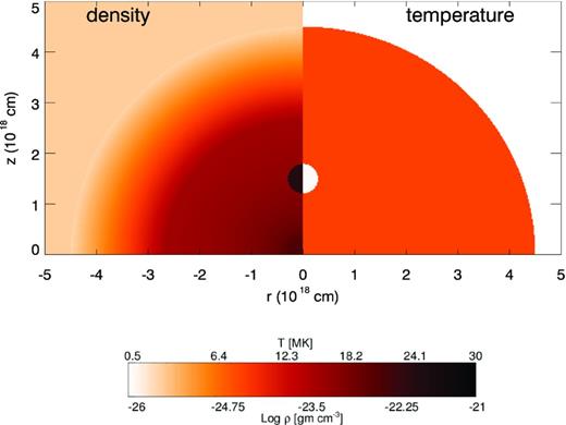
Density (left-hand panel) and temperature (right-hand panel) 2D cross-sections through the (r, z) plane showing an example of the initial conditions of our simulations (namely R1/3 − CHI20, see Table 1). The system consists of an expanding spherically symmetric distribution of ejecta where we place a dense, isobaric and spherical knot. In this case the knot is 20 times denser than the surrounding ejecta.
Physical parameters of the model setups (see Section 2). TC-RL indicates that the simulations were performed by including thermal conduction and radiative losses. In all the setups the initial radius of the ejecta is R|${^{0}_{ej}}$| = 4.5 × 1018 cm.
| Model setup | χ | Rs (cm) | TC-RL |
|---|---|---|---|
| R1/3 − CHI10 | 10 | 1.5 × 10¹⁸ | No |
| R1/3 − CHI10 − TR | 10 | 1.5 × 10¹⁸ | Yes |
| R1/3 − CHI20 | 20 | 1.5 × 10¹⁸ | No |
| R1/3 − CHI20 − TR | 20 | 1.5 × 10¹⁸ | Yes |
| R1/3 − CHI50 | 50 | 1.5 × 10¹⁸ | No |
| R1/6 − CHI50 | 50 | 0.75 × 10¹⁸ | No |
| R1/6 − CHI50 − TR | 50 | 0.75 × 10¹⁸ | Yes |
Vela SNR is the result of a core-collapse SN and we expect the ambient medium to be ‘perturbed’ by the wind residuals of the massive progenitor star. However, we assume for simplicity a uniform ambient medium as in WC02, since here we are not interested in modelling the details of the remnant evolution. The final (i.e. after 11 000 yr, the age of the Vela SNR; Taylor, Manchester & Lyne 1993) radius of the remnant strongly depends on the choice of the ambient density value, nISM. We set nISM = 0.5 cm−3, because with this value (and with the chosen values of K, Mej, nISM, b and m), the radius of the shell after 11 000 yr is Rshell ∼ 5.4 × 1019 cm, in good agreement with the observed radius of the Vela SNR that ranges between 5 × 10¹⁹ and 5.5 × 1019 cm (by assuming a distance of 250 pc, in agreement with Bocchino, Maggio & Sciortino 1999 and Cha, Sembach & Danks 1999).
Our model solves the time-dependent compressible fluid equations of mass, momentum and energy conservation. In three cases, we ran the same simulation with/without thermal conduction and radiative cooling inside our system, as shown in Table 1. As for thermal conduction, we considered both the Spitzer and the saturated regimes, while radiative losses (that can play an important role in the Vela SNR, as shown by Miceli et al. 2006) were computed for an optically thin thermal plasma. The model equations are described in Miceli et al. (2006, equations 1– 5 therein) and were solved by using the flash code (Fryxell et al. 2000).
The computational domain extends over 8 × 1019 cm in the r and z directions. We use axisymmetric boundary conditions at r = 0, reflection boundary conditions at z = 0 and zero-gradient (outflow) boundary conditions (for |${\boldsymbol v}$|, ρ, and p) elsewhere. We trace the motion of the ejecta material and of the shrapnel with passive tracers.2 Considering the large range in spatial scales of our simulations, we exploited the adaptive mesh capabilities of the flash code by adopting up to 10 nested levels of resolution (the resolution increases by a factor of 2 at each level). The refinement/derefinement criterion (Lohner 1987) follows the gradients of density, temperature and tracers. The finest spatial resolution is 1.95 × 1016 cm at the beginning of the simulation, therefore there are 230 computational cells per initial radius of the ejecta and ∼10 cells per initial radius of the shrapnel (that varies in the range 1.8–2.9 × 1017 cm). Because of the expansion of the system, the resolution is reduced by a factor of 2 after 2500 yr. We verified that by changing the resolution of our simulations by a factor of 2, the results do not change significantly (see Appendix A for further details).
3 RESULTS
3.1 Evolution of the system
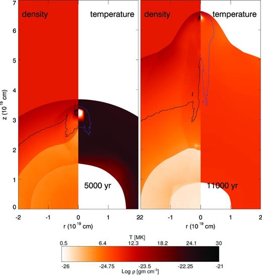
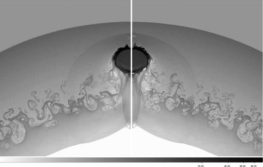
We first focus on simulation R1/3 − CHI20. Fig. 2 shows the 2D cross-sections through the (r, z) plane of temperature and density at different evolutionary stages of the R1/3 − CHI20 simulation. The left-hand panel shows the system 5000 yr after the beginning of the simulation,3 when the shrapnel interacts with the intershock region. Rayleigh–Taylor and Richtmyer–Meshkov instabilities are visible as finger-like structures both in the density and temperature maps. At this stage, the knot is partially eroded by the hydrodynamic instabilities and evolves towards a core-plume structure. The core of the knot, however, is still significantly overdense with respect to the surrounding shocked ejecta. The right-hand panel of Fig. 2 shows the shrapnel at t = 11 000 yr, with its characteristic supersonic bow shock protruding beyond the SNR main shock.
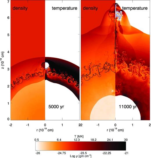
Left-hand panel: density (left) and temperature (right) 2D cross-sections through the (r, z) plane showing simulation R1/3 − CHI20 at t = 5000 yr. The black/blue contours enclose the computational cells consisting of the original ejecta/shrapnel material by more than 90 per cent. The colour bar indicates the logarithmic density scale and the linear temperature scale. Right-hand panel: same as left-hand panel, for t = 11 000 yr.
WC02 found that ejecta knots with density contrast χ ≤ 100 are rapidly fragmented and decelerated in the intershock region and do not even reach the main shock front (these effects being more dramatic for small clumps). Nevertheless, we notice that the value of χ in WC02 refers to the onset of the interaction between the knot and the reverse shock and that χ is not constant during the evolution of the system. In the ‘free’ expansion phase, the density of the shrapnel does not drop down uniformly (as that of the other ejecta does) and the shrapnel undergoes both diffusion and expansion. Fig. 3 presents a close-up view of the shrapnel density structure at t = 2500 yr, showing that, while the outer parts of the knot diffuse and mix with the expanding ejecta, its central core remains much denser. The density of the core of the clump drops down much more slowly than that of the spherically expanding ejecta. Therefore, the inhomogeneous rarefaction of the knot makes the density contrast between the core of the shrapnel and the expanding ejecta higher, and χ rapidly increases until the shrapnel reaches the reverse shock. We computed χ during the expansion phases, by calculating the shrapnel density, |$\overline{\rho _s}$|, as the average of the density in all the computational cells where the shrapnel content is >90 per cent.4 We then divided |$\overline{\rho _s}$| by the ejecta density (along the r-axis) at the same distance from the origin as the shrapnel centre. Fig. 4 shows the evolution of χ as a function of time for the R1/3 − CHI20 simulation. The figure shows that the ejecta knot reaches χ > 100 as it approaches the reverse shock, hence our results are in agreement with those of WC02. Our model shows that a knot that was only 20 times denser than the surrounding ejecta (at the beginning of the simulations) can reach the SNR main shock without being fragmented in the intershock region and can produce protrusions that are similar to those actually observed in the Vela SNR.
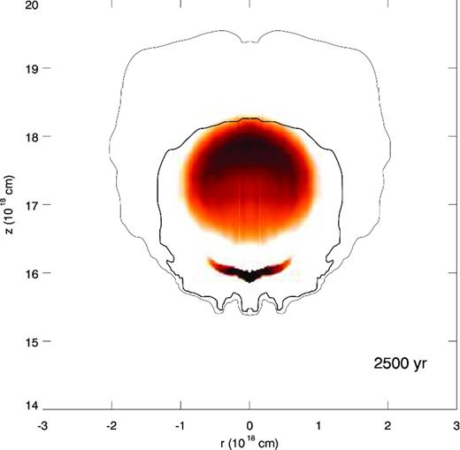
Density 2D cross-sections through the (r, z) plane for model R1/3 − CHI20 at t = 2500 yr. The colour scale increases linearly between 10−22 and 2 × 10⁻²² g cm−3. The contours enclose the computational cells consisting of the original shrapnel material by more than 99 per cent (bold line) and 50 per cent (narrow line).
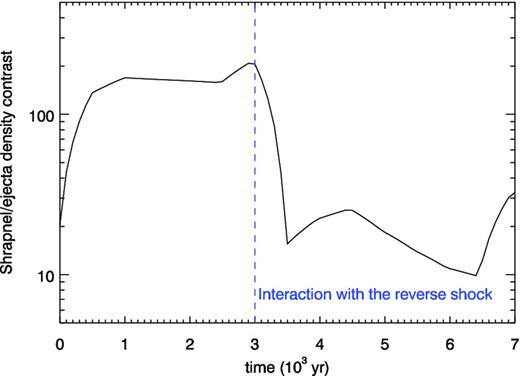
Temporal evolution of the shrapnel/ejecta density contrast for model R1/3 − CHI20. The blue horizontal line marks the beginning of the interaction between the shrapnel and the SNR reverse shock.
3.2 Effects of thermal conduction and radiative cooling
For a characteristic structure with size l ∼ 4 × 1018 cm, particle density n = 0.8 cm−3, Atwood number |$\overline{A}\sim 0.44$|, Δv ∼ 2 × 107 cm/s, T ∼ 1.3 × 10⁷ K (similar to that shown in Fig. 2), τinst ∼ 1.4τcond ∼ 2000 yr. Therefore, the thermal conduction diffusive processes develop faster than the hydrodynamic instabilities and density and temperature inhomogeneities are smoothed out before they can grow.
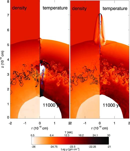
The evolution of the position of the shrapnel head and the protrusion it produces to the remnant shock front are similar to those obtained without including thermal conduction and radiative cooling. Nevertheless, the shrapnel evolution is remarkably different from that obtained in the pure hydrodynamic (HD) simulations. In particular, as shown by the blue contours in Fig. 5, the ejecta knot is elongated along its direction of motion and rapidly assumes a cometary shape, characterized by a prominent tail which is rich in shrapnel material. After t = 11 000 yr, shrapnel material is present at ∼10 pc away from the shrapnel head. Moreover, the shrapnel material is efficiently heated by thermal conduction with the surrounding shocked ejecta. Let MXshra be the mass of the plasma in the computational cells consisting of the original shrapnel material by more than 90 per cent and having a temperature higher than 106 K (and therefore emitting thermal X-rays). Fig. 6 shows the evolution of MXshra as a function of time for the simulations R1/3 − CHI20 − TR and R1/3 − CHI20. When thermal conduction is at work, ∼90 per cent of the original shrapnel mass is heated up to X-ray emitting temperature at t = 11 000 yr (i.e. at the age of the Vela SNR), while if thermal conduction in inhibited, only 50 per cent of the original mass has temperature higher than 106 K. Fig. 6 also shows the amount of X-ray mass beyond the shock front. In the pure HD simulation, the hot shrapnel material is all beyond the SNR shock front. In the R1/3 − CHI20 − TR simulation, only part of the X-ray emitting shrapnel is beyond the shock front and there is a significant fraction of the ejecta knot material (the shrapnel tail) that is inside the SNR shell and that is expected to emit thermal X-rays (see Section 4).
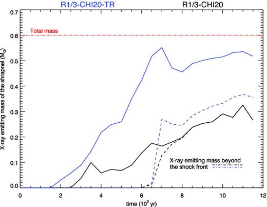
Temporal evolution of MXshra (mass of the plasma in the computational cells consisting of the original shrapnel material by more than 90 per cent and having a temperature higher than 106 K) for the simulations R1/3 − CHI20 − TR (blue curves) and R1/3 − CHI20 (black curves). The dashed lines indicate the part of MXshra that protrudes beyond the SNR shock front.
We point out that in SNRs the efficiency of thermal conduction can be significantly reduced by the presence of the magnetic field (which is not taken into account in our model). If we assume an organized ambient magnetic field, the thermal conduction is anisotropic, because the conductive coefficient in the direction perpendicular to the field lines is several orders of magnitude lower than that parallel to the field lines, which coincides with the Spitzer coefficient κ(T). The effects of the magnetic-field-oriented thermal conduction in the interaction between shocks and dense clump have been investigated in detail in Orlando et al. (2008). Because of the high beta of the plasma, the magnetic field lines are expected to envelope the hydrodynamic fingers thus hampering the thermal conduction with the surrounding material. At the same time, the magnetic field is expected to be trapped at the top of the ejecta clumps, and this yields to an increase of the magnetic pressure and field tension which limits the growth of hydrodynamic instabilities (see O12 and Sano et al. 2012). The basic physics of the interaction between the ejecta knots and the SNR shocks is similar to that for the interaction of planar shocks with an interstellar cloud (e.g. WC02) and it has been shown that, in this case, simulations including thermal conduction in an unmagnetized plasma and pure HD simulations are limiting cases that encompass the results obtained with different configurations of the magnetic field (Orlando et al. 2008). We can then conclude that our simulations provide the two extreme cases that bracket all the possible intermediate scenarios.
3.3 Effects of the initial conditions
We study the effects of the initial conditions on the shrapnel evolution with different simulations, as shown in Table 1. In particular, we explored two different initial positions of the shrapnel in the ejecta profile (Rs = 1/6 R|${^{0}_{ej}}$|, 1/3 R|${^{0}_{ej}}$|) and three different density contrasts (χ = 10, 20, 50).
In agreement with WC02, we found that shrapnel formed in the inner ejecta layers (i.e. those that reach the reverse shock later) produce smaller protrusions. In particular, an ejecta knot originating at Rs = 1/6 R|${^{0}_{ej}}$| does not even reach the SNR shock in the time spanned by our simulations. Therefore, our model indicates that Shrapnel A–F (all protruding well beyond the Vela main shock) originated in more external layers. Left-hand panel of Fig. 7 shows the 2D cross-sections through the (r, z) plane of temperature and density at the age of the Vela SNR for the R1/6 − CHI50 simulation. In this case, the knot is well within the intershock region, even though its initial density contrast (χ = 50) was higher than that of the R1/3 − CHI20 run. However, our models of knots originating at Rs = 1/3 R|${^{0}_{ej}}$| clearly show that denser shrapnel produce deeper protrusions and are more stable against the fragmentation and the deceleration induced by the hydrodynamic instabilities in the intershock region (as in WC02).5 Fig. 7, right-hand panel, shows the 2D cross-sections through the (r, z) plane of temperature and density at the age of the Vela SNR for the R1/3 − CHI50 simulation. As expected, the shrapnel head is much further away from the SNR shell than in the R1/3 − CHI20 case (shown in the right-hand panel of Fig. 2). We computed the time evolution of χ for the R1/3 − CHI50 run by following the procedure described in Section 3.1. We found that, in this case, the ejecta knot reaches the reverse shock with a very high density contrast (χ > 1000, see Fig. 8), thus producing a very prominent protrusion in the SNR.
Left-hand panel: density (left) and temperature (right) 2D cross-sections through the (r, z) plane showing simulation R1/6 − CHI50 at t = 11 000 yr. The black/blue contours enclose the computational cells consisting of the original ejecta/shrapnel material by more than 90 per cent. The colour bar indicates the logarithmic density scale and the linear temperature scale. Right-hand panel: same as left-hand panel, for simulation R1/3 − CHI50.
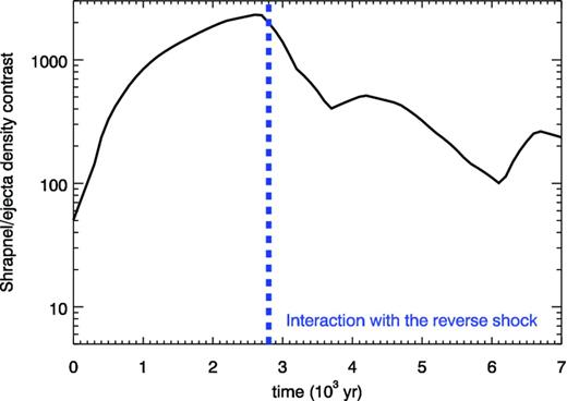
Fig. 9 shows the position of the shrapnel head (in units of the shell radius) as a function of time for all our simulations. Fig. 9 also shows the projected positions of Shrapnel A–D (Aschenbach et al. 1995) and of the ejecta knots FilE and RegNE (Miceli et al. 2008) with respect to the position of the shock front in the Vela SNR. These values were calculated by approximating the Vela SNR as a circular shell with angular radius 211 arcmin and centre with coordinates | $\alpha _{\rm J2000} = 8^{\rm h} 36^{\rm m} 19^{\rm s}_{.}8 \delta _{\rm J2000} = - 45^{\circ} 24^{\prime} 45^{\prime \prime}$|. Models including the effects of radiative cooling and thermal conduction (blue curves in Fig. 9) do not provide significant differences with respect to pure HD models (black curves) in terms of the shrapnel position.

Position of the shrapnel head (in units of the shell radius Rshell) as a function of time for all the simulations listed in Table 1. The black curves indicate pure hydrodynamic models, while the blue curves indicate simulations including thermal conduction and radiative cooling. The dashed/solid/thick lines indicate χ = 10/20/50, respectively. The red diamonds show the projected positions of Shrapnel A–D (Aschenbach et al. 1995) and of the ejecta knots FilE and RegNE (Miceli et al. 2008).
By considering all the simulations with Rs = 1/3 R|${^{0}_{ej}}$|, we find that the position of the head of the knot, Rh, after ∼11 000 yr ranges between ∼1.1 Rshell (for χ = 10) and ∼1.4 Rshell (for χ = 50). These values are similar to those observed for Shrapnel B, C, and D.
Shrapnel A, E and F (Shrapnel E and F are not shown in Fig. 9) instead have Rh = 1.57 Rshell, Rh = 1.88 Rshell and Rh = 1.91 Rshell, respectively. These values are much larger than those obtained in our simulations. Our results clearly suggest that these large distances from the shell can be produced by ejecta knots originating in outer ejecta layers. An alternative possibility is that the original density contrast for these shrapnel was >50. Nevertheless, Fig. 9 shows that the final position of an ejecta clump is more sensitive to its initial position and depends only weakly on χ. In fact, by varying the initial position of the knot by a factor of 2, we found that its final position varies approximately by the same factor, while a variation of the initial density contrast by a factor of 5, only determines a 30 per cent variation in the final position. Therefore, it is more likely that Shrapnel A, E and F were produced at |$R_s>1/3\ R^{0}_{{\rm {\rm e} j}}$|.
The two simulations with Rs = 1/6 R|${^{0}_{ej}}$| show that the ejecta knots originating in the inner ejecta layers do not reach the forward shock, even for the highest density contrast (χ = 50). The position of the head of the knot predicted by our simulations is in agreement with that observed for FilE (Miceli et al. 2008). X-ray emitting ejecta knots have been observed, in projection, inside the Vela SNR shell (e.g. RegNE and FilE; Miceli et al. 2008). However, we point out that the actual position of these ‘internal’ shrapnel can be well outside the SNR shell, and therefore the values reported in Fig. 9 might be considered as lower limits.
4 DISCUSSIONS AND CONCLUSIONS
The structure of the ejecta in a SNR contains the imprint of the metal-rich layers inside the progenitor star, and may help to understand the processes occurring in the latest stage of stellar evolution. We performed a set of hydrodynamic simulations to study the evolution of the ejecta knots in the Vela SNR.
We found that moderately overdense clumps (initial density contrast χ ∼ 10) can produce protrusions in the SNR shell similar to those observed for the Vela shrapnel. WC02 found that only clumps that reach the reverse shock with density contrast χ ≥ 100 can reach the main shock front and produce significant protrusions. This criterion is fulfilled in all our simulations. In fact, the (initially) moderately overdense clump experiences diffusion in the ‘free’ expansion phase, and, while its outer parts mix with the surrounding ejecta, its central core remains much denser. This inhomogeneous rarefaction makes the density contrast between the core of the shrapnel and the expanding ejecta higher as the remnant evolves, and χ reaches values ∼100–1000 at the interaction with the reverse shock.
In particular, a knot with initial χ = 20 and Rs = 1/3 R|${^{0}_{ej}}$| (simulations R1/3 − CHI20 and R1/3 − CHI20 − TR) can explain the observed features associated with the Vela Shrapnel D. Fig. 10 shows the ROSAT All-Sky Survey image of the Vela Shrapnel D in the 0.1–2.4 keV energy band, compared with a synthesis of the X-ray emission in the 0.1–2.4 keV band derived from the R1/3 − CHI20 − TR simulation at 11 000 yr. The synthesized X-ray map has been obtained as in Miceli et al. (2006): we produced the 3D map of the emission measure and temperature in the Cartesian space (x′, y′, z′), where the y′-axis corresponds to the direction of the line of sight and is perpendicular to the (r, z) plane. We derived the distribution EM(x′, z′) versus T(x′, z′) by considering all the contributions along the line of sight, for each (x′, z′). We then synthesized the map of the X-ray emission using the mekal spectral code (Mewe, Gronenschild & van den Oord 1985; Mewe, Lemen & van den Oord 1986; Liedahl, Osterheld & Goldstein 1995), assuming a distance of 250 pc, and an interstellar column density NH = 2 × 1020 cm−2. Finally, we degraded the spatial resolution of the synthesized X-ray map to match the resolution of the ROSAT image and randomized the map by assuming Poisson statistics for the counts in each image bin.
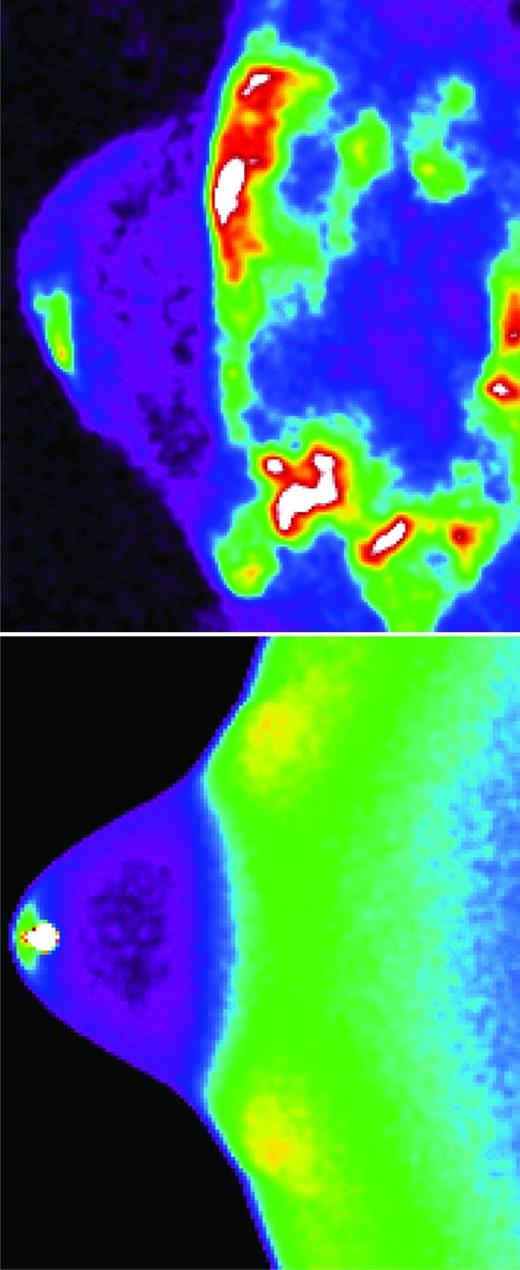
Upper panel: ROSAT All-Sky Survey image of Vela Shrapnel D in the 0.1–2.4 keV energy band. The bin-size is 1.5 arcmin and the image has been smoothed through a convolution with a Gaussian with σ = 3 pixels. North is up and East is to the left. Lower panel: synthesized X-ray emission in the 0.1-2.4 keV band for the simulation R1/3 − CHI20 − TR at t = 11 000 yr (see Section 4).
Fig. 10 shows that the bright X-ray spot at the apex of the shrapnel bow shock and the enhanced X-ray luminosity at the base of the protrusion can be explained by our model as local enhancements of the plasma emission measure. The overall shape of the observed features is also reproduced by our model. Moreover, the mass of the X-ray emitting shrapnel predicted by our model is in agreement with that measured for Shrapnel D. In fact, it has been estimated that the X-ray emitting mass (considering only the bulge above the Vela SNR bow shock) is ∼0.1 M⊙ (Katsuda & Tsunemi 2005), i.e. the same order of magnitude as that obtained in our simulation (see dashed curves in Fig. 6). Vela Shrapnel D is therefore consistent with being originated by an ejecta knot 20 times denser than the surrounding ejecta and initially located at 1/3 R|${^{0}_{ej}}$|. As shown in Fig. 9, we found a degeneracy in the space of the initial parameters, and similar results can be obtained also by enhancing/decreasing the density contrast and decreasing/increasing the initial distance of the knot to the explosion centre. However, as explained in Section 3.3, the final position of the shrapnel is much more sensitive to its initial position in the ejecta profile. In conclusion, according to our model, the original position of Shrapnel D should not differ much from 1/3 R|${^{0}_{ej}}$|.
As shown in Section 3.3, our model suggests that Shrapnel B, C and D were all originated at ∼ 1/3 R|${^{0}_{ej}}$|. This conclusion is in agreement with the results of X-ray data analysis that show that Shrapnel B and D have similar abundance patterns (Katsuda & Tsunemi 2005; Yamaguchi & Katsuda 2009). The fragment RegNE, which appears inside the Vela shell, has similar abundances as Shrapnel D (Miceli et al. 2008) and its position is compatible with an origin in the same layer where Shrapnel B, C and D were generated.6
In Section 3.3, we also pointed out that it is highly unlikely that Shrapnel A originated in the same ejecta layer as Shrapnel D. Indeed, the abundance patterns observed in Shrapnel A are remarkably different from that observed in Shrapnel B and D (Katsuda & Tsunemi 2006), thus suggesting a different location of this knot in the ejecta profile. Nevertheless, the Si:O ratio is much higher in Shrapnel A than in Shrapnel D and this indicates that Shrapnel A comes from a region of the progenitor star below that of the Shrapnel D (e.g. Tsunemi & Katsuda 2006), at odds with our predictions. As explained above, an unrealistically high initial χ is required for an inner shrapnel to overcome outer knots, if we assume that the initial velocity profile of the ejecta increases linearly with their distance from the centre. A possible solution for this puzzling result is that the Si burning layer (or part of it) has been ejected with a higher initial velocity, e.g., as a collimated jet. It is noteworthy to remark that in other core-collapse SNRs the Si-rich ejecta may show a very peculiar jet–counterjet structure. The well-known case of Cas A has been studied in detail thanks to a very long Chandra observation (Hwang et al. 2004) showing a jet (with a weaker counterjet structure) composed mainly of Si-rich plasma. Laming et al. (2006) have performed X-ray spectral analysis of several knots in the jet and concluded that the origin of this interesting morphology is due to an explosive jet and it is not arising because of an interaction with a cavity or other ISM/CSM peculiar structure. Therefore, a jet origin for the Si-rich knots is sound.
Finally, we investigated the effects of thermal conduction, finding that it determines an efficient ‘evaporation’ of the ejecta knot and accelerate its mixing with the surrounding medium. Moreover, it affects the shrapnel morphology, producing the formation of a long, metal-rich tail. Enhanced metallicities have been observed in the tails of Shrapnel A, B and D and the abundance analysis performed on the X-ray spectra clearly suggests an efficient mixing of the ejecta knots with the surrounding medium (Katsuda & Tsunemi 2005, 2006; Yamaguchi & Katsuda 2009). These results are in qualitative agreement with our findings. A quantitative comparison between models and observations requires a forward modelling approach, consisting in the synthesis of the X-ray spectra from the simulations and a detailed comparison between the synthesized observables and the corresponding observations (e.g. through a spatially resolved spectral analysis, as in Miceli et al. 2006, e.g.). Moreover, it will also be important for future models to include some seed magnetic fields in the simulations to study how tangled the field becomes and what this implies for thermal conduction. These further studies are beyond the scope of this paper.
In conclusion, our hydrodynamic modelling of ejecta knots in the Vela SNR allowed us to find: (i) the observed shrapnel can be the results of moderate density inhomogeneities in the early ejecta profile; (ii) the evolution of a shrapnel in the SNR is very sensitive to its initial position and depends much less (but does depend) on the initial density contrast; (iii) thermal conduction plays an important role and explains the efficient mixing of the ejecta knots observed in X-rays.
We thank the anonymous referee for their constructive suggestions to improve the paper. The software used in this work was in part developed by the DOE-supported ASC/Alliance Center for Astrophysical Thermonuclear Flashes at the University of Chicago. The simulations discussed in this paper have been performed on the HPC facility at CINECA, Italy, and on the GRID infrastructure of the COMETA Consortium, Italy.
The size of the clump varies accordingly.
Both tracers have zero mass and do not modify the dynamics of the system.
In the following, all the ages will be reckoned from the beginning of our simulations. We remind the reader that our initial condition corresponds to ∼240 yr after the SN explosion.
These cells are closer to the centre of the knot, and are less affected by the diffusion.
In our runs, higher values of χ correspond to smaller values of the shrapnel cross-section (given that the shrapnel mass is fixed to 1.19 × 1033 g in all our simulations), and this concurs in making the knot a more penetrating bullet.
In this case, its projected distance from the centre of the SNR must be much smaller than its actual distance.
REFERENCES
APPENDIX A TEST ON SPATIAL RESOLUTION
As explained in Section 2.1, the spatial resolution of our simulations is reduced by a factor of 2 at t > 2500 yr. To check whether this resolution is sufficient to capture the basic evolution of the system, we repeated simulation R1/3 − CHI20 by maintaining the finest level of resolution at its initial value (1.95 × 1016 cm, hereafter simulation R1/3 − CHI20 − hiRES) for the whole run. We verified that simulations R1/3 − CHI20 and R1/3 − CHI20 − hiRES yield very similar results and all the quantities discussed in the paper (position of the shrapnel as a function of time, X-ray emitting mass of the shrapnel, etc.) do not change significantly. Fig. A1 shows the 2D cross-sections of the density through the (r, z) plane obtained for simulations R1/3 − CHI20 and R1/3 − CHI20 − hiRES at t = 5000 yr. This evolutionary stage is the most critical, since the system is still relatively small and the ejecta knots interact with the hydrodynamic instabilities in the intershock region. Fig. A1 clearly proves that simulation R1/3 − CHI20 already provides a very accurate description of the system and run R1/3 − CHI20 − hiRES does not introduce any major differences.
Density 2D cross-sections through the (r, z) plane for simulation R1/3 − CHI20 (left-hand panel) and R1/3 − CHI20 − hiRES (right-hand panel) at t = 5000 yr. The colour bar indicates the logarithmic density scale and ranges between 10−25 and 10−22 g cm−3.
