


Abstract
Massive neutrinos make up a fraction of the dark matter, but due to their large thermal velocities, cluster significantly less than cold dark matter (CDM) on small scales. An accurate theoretical modelling of their effect during the non-linear regime of structure formation is required in order to properly analyse current and upcoming high-precision large-scale structure data, and constrain the neutrino mass. Taking advantage of the fact that massive neutrinos remain linearly clustered up to late times, this paper treats the linear growth of neutrino overdensities in a non-linear CDM background. The evolution of the CDM component is obtained via N-body computations. The smooth neutrino component is evaluated from that background by solving the Boltzmann equation linearized with respect to the neutrino overdensity. CDM and neutrinos are simultaneously evolved in time, consistently accounting for their mutual gravitational influence. This method avoids the issue of shot noise inherent to particle-based neutrino simulations, and, in contrast with standard Fourier-space methods, properly accounts for the non-linear potential wells in which the neutrinos evolve. Inside the most massive late-time clusters, where the escape velocity is larger than the neutrino thermal velocity, neutrinos can clump non-linearly, causing the method to formally break down. It is shown that this does not affect the total matter power spectrum, which can be very accurately computed on all relevant scales up to the present time.
INTRODUCTION
The determination of neutrino masses lies on the boundary between particle physics, astrophysics and cosmology. Atmospheric and solar neutrino oscillations have allowed the measurement of two mass-squared differences Δm212 ≡ m22 − m21 = 7.54+ 0.46− 0.39 × 10− 5 and |Δm213| ≡ |m32 − (m21 + m22)/2| = 2.43+ 0.12− 0.16 × 10− 3 eV2 (central values and 2σ error bars from Fogli et al. 2012). These measurements do not allow us to pin down the individual neutrino masses, nor their hierarchy, since only the absolute value of Δm213 is measured – note, however, that next-generation oscillation experiments such as NOVA1 aim to distinguish the neutrino hierarchy through second-order mixing effects. Current β-decay experiments imply an upper limit on the individual neutrino mass mν ≲ 2 eV (Kraus et al. 2005), and future experiments like KATRIN (KArlsruhe TRItium Neutrino experiment) should lower this limit by an order of magnitude (Eitel 2005).
Cosmological probes are sensitive to the absolute mass of neutrino species (see, for example, Lesgourgues & Pastor 2006 and Wong 2011 for recent reviews), and so far provide the tightest limits on the total neutrino mass Mν ≡ ∑mν ≡ m1 + m2 + m3, at the level of a few tenths of electron volts (eV). Increasingly sensitive future experiments aim to reach levels of precision at which a total neutrino mass ∑mν ∼ 0.1 eV or lower would be detectable (we refer the reader to Abazajian et al. 2011 for a recent compilation of current constraints and forecasts). Ultimately, the neutrino hierarchy may even be within reach (Takada, Komatsu & Futamase 2006; Jimenez et al. 2010).
Massive neutrinos affect the growth of perturbations through two effects. First, they change the background evolution. For a total neutrino mass less than a few eV, neutrinos are still relativistic at the time of matter-radiation decoupling but non-relativistic today. At fixed total density of non-relativistic matter today, the epoch of matter-radiation equality is moved to later times as the neutrino mass is increased. If one holds the density of baryons and CDM fixed instead, the angular-diameter distance and time of matter – dark energy equality are changed for different neutrino masses. In each case, the cosmic microwave background (CMB) anisotropy power spectrum is affected (Lesgourgues & Pastor 2006; Wong 2011), which has allowed CMB observations to set what is perhaps the most robust constraint on the neutrino mass, ∑mν < 1.3 eV (Komatsu et al. 2011). Upcoming data from the Planck satellite is expected to lower this bound by a factor of 2 (Planck Collaboration 2005; Abazajian et al. 2011).
The second effect of massive neutrinos is to slow down the growth of structure on scales smaller than their free-streaming length. This effect has long been understood in the linear regime (Bond, Efstathiou & Silk 1980; Bond & Szalay 1983; Ma & Bertschinger 1995; Lesgourgues & Pastor 2006 and references therein), and is implemented in all modern Boltzmann codes (see for example Lewis & Challinor 2002; Lesgourgues & Tram 2011). For a total neutrino mass of a few tenths of eV, this effect becomes manifest at scales ≲100h−1 Mpc and gets stronger in the non-linear regime at scales of a few tenths to a few tens of Mpc (Lesgourgues & Pastor 2006).
Combined with CMB anisotropy measurements, various probes of the matter distribution have already constrained the total neutrino mass to ∑mν ≲ 0.2–0.3 eV. These include galaxy surveys such as SDSS (Sloan Digital Sky Survey; de Putter et al. 2012; Xia et al. 2012), cosmic shear surveys such as CFHT-LS (Canada-France-Hawaii Telescope Legacy Survey; Ichiki, Takada & Takahashi 2009), Lyman α forest measurements (Seljak, Slosar & McDonald 2006; Viel, Haehnelt & Springel 2010) and galaxy cluster surveys (Vikhlinin et al. 2009). As the survey samples grow larger, the sensitivity to the neutrino mass is expected to reach ∑mν ∼ 0.1 eV (Abazajian et al. 2011) or even lower (see Takada et al. 2006 for a detailed Fisher-matrix forecast of the constraining power of future high-redshift surveys). In addition, future measurements of CMB lensing (Hall & Challinor 2012) and 21 cm surveys (Mao et al. 2008) have the potential to reach yet lower bounds. Massive neutrinos also affect the growth of haloes (Brandbyge et al. 2010; Marulli et al. 2011).
Each one of the aforementioned methods has its own advantages and limitations. Systematic errors may arise from using biased tracers of the underlying density field, from difficulties in modelling complex baryonic physics or from foreground contamination. In addition, this level of precision requires an accurate modelling of corrections from non-linear structure growth. Here we focus on the latter problem. Cosmological neutrinos only interact gravitationally and, because of their large thermal velocities, effectively constitute a hot dark matter (HDM) component. While it poses significant practical difficulties, the non-linear clustering of massive collisionless particles is now a relatively well-understood problem. The growth of pure cold dark matter (CDM) structure can be computed through collisionless N-body simulations, whose accuracy is limited primarily by available computational resources, which have been steadily increasing over time (see e.g. fig. 1 of Dehnen & Read 2011). By contrast, the effect of neutrinos on the non-linear growth of matter perturbations has only recently been investigated in depth. This delicate problem has been approached from two angles. On the one hand, extensions to perturbation theory allow for semi-analytic calculations of the CDM power spectrum in the weakly non-linear regime. Combined with a linear treatment of neutrinos, such methods can reach a few per cent accuracy up to k ∼ 1 h Mpc−1 at high redshifts (z ≳ 2) (Saito, Takada & Taruya 2008, 2009; Wong 2008; Lesgourgues et al. 2009). Shoji & Komatsu (2009) go beyond linear theory for neutrinos and solve for both the CDM and neutrino overdensities to third order in perturbation theory, making however the simplifying assumption that neutrinos can be described by an ideal fluid with a constant Jeans scale. Hannestad, Haugbølle & Schultz (2012) incorporated neutrinos into N-body simulations using a similar fluid approach.
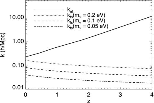
Non-linear scale (solid) and free-streaming scales for various neutrino masses, as a function of redshift.
On the other hand, the ‘exact’ solution to the problem of CDM+neutrino clustering can in principle be obtained from N-body simulations where both CDM and neutrinos are simulated as particles. This approach was recently taken by Brandbyge et al. (2008), Viel et al. (2010) and Bird, Viel & Haehnelt (2012) (see also references therein for earlier works). The main limiting factor of such an approach is numerical: since neutrinos do not significantly cluster below their free-streaming scale, their power spectrum on small scales is dominated by shot noise for any reasonable number of simulated particles,2 increasingly so for lower neutrino masses and at earlier times. A vast amount of computational power and memory is therefore wasted to extract a small amount of information on the actual neutrino clustering. In order to bypass the shot noise issue, Brandbyge & Hannestad (2009) included neutrino perturbations in Fourier space, while still treating the CDM component as particles in N-body simulations. The density field of their neutrino component was only computed using linear theory, however, and did not account consistently for non-linear CDM perturbations sourcing the gravitational potential in which neutrinos evolve (Bird et al. 2012). Recently, Brandbyge & Hannestad (2010) suggested a hybrid method, where neutrinos are initially treated using the Fourier method with linear theory, and converted to particles as time progresses. One of the remaining sources of errors of this implementation is that the Fourier-space part does not account for the non-linear growth of gravitational potentials in the neutrino evolution.
The aim of this work is to close this gap and provide an efficient method for accurately computing the effect of massive neutrinos on the non-linear matter power spectrum, with a minimal modification to well-tested pure CDM N-body simulation methods. To do so, we follow the CDM with the tree-PN N-body code gadget-3 (Springel 2005; Viel et al. 2010), and compute analytically the linearized neutrino overdensity sourced by the full gravitational potential. The CDM and neutrinos are evolved simultaneously and self-consistently, accounting for their mutual gravitational influence. Our method is therefore semilinear, in the sense that we account exactly for the non-linear growth of CDM overdensities and gravitational potentials, but effectively use a linear transfer function to obtain the neutrino overdensity from the gravitational potential. For neutrinos of the mass allowed by current data, our implementation is sufficient on its own for a complete description of the matter power spectrum up to the present time, and, for z ≥ 1, the neutrino power spectrum as well. It only fails to resolve neutrino clustering in the most massive galaxy clusters, in which neutrinos do cluster non-linearly (Ringwald & Wong 2004); however, it should be easy to perform zoomed simulations of these clusters using our method as a base. An ancillary advantage of our implementation is that it can easily be added into an N-body code as a small ‘patch’ and does not require running an independent Boltzmann code in parallel. Furthermore, our code can easily include the exact contribution of neutrinos to the background expansion, and the effect of the neutrino hierarchy, which are problematic or expensive to include in particle implementations. It can be applied to regimes where shot noise severely limits the reliability of the particle method, such as low neutrino masses, the 21cm forest or large-volume galaxy mock catalogue simulations. Perhaps the most important property of our code is that it allows massive neutrinos to be included into simulations with negligible cost in CPU and memory, and with no loss of accuracy. Thus, it can be useful for interpreting the results of essentially any probe of large-scale structure, including CMB lensing, the Lyman α forest, weak lensing experiments or galaxy surveys (Cooray 1999; Kaplinghat, Knox & Song 2003; Wang et al. 2005; Takada et al. 2006; Gratton, Lewis & Efstathiou 2008; Ichiki et al. 2009; Schlegel, White & Eisenstein 2009; Vallinotto et al. 2009; Beaulieu et al. 2010; Carbone et al. 2011).
This paper is organized as follows. In Section 2, we define our notation and discuss characteristic scales and the regime of validity of our main approximation. We derive our main equations in Section 3. The practical interfacing with our N-body code is detailed in Section 4. We describe our results and compare them against other methods in Section 5. We discuss potential applications of our method in Section 6 and conclude in Section 7.
NOTATION, CHARACTERISTIC TIME-SCALES AND LENGTH-SCALES
Notation
Relativistic to non-relativistic transition
Free-streaming scale
We therefore expect the neutrino component to be linearly clustered on all scales for masses below the current upper limit: for k < knl neutrinos cluster at most like the CDM, which is itself linearly clumped. For k > knl > kfs, the neutrino power per logarithmic interval is a decreasing function of k.
This argument motivates our use of linear theory for the neutrino component. However, this does not give the full physical picture of neutrino clustering: the slowest neutrinos may in fact significantly cluster in massive haloes. Before moving to the core of our calculation, we first discuss in which conditions it may break down.
Neutrino capture in massive haloes
Let us emphasize that although the crossing time of a neutrino in a massive halo is significantly shorter than the Hubble time (for the fiducial values of equation 16, Hδt ≈ 1/40 at z = 0), the relevant comparison is not of Hδt with unity but rather with the small ratio v2/ϕ (also ≈1/40 for our adopted fiducial values): even a small relative effect due to the change of the potential on a Hubble time-scale may translate into an order unity effect on the pre-entry velocity and prevent the neutrino from escaping the halo.
The analysis presented here is of course very simplified, for we have used an idealized (and unphysical) profile for the gravitational potential. Moreover, in reality there is no sharp boundary in momentum space between linear behaviour and strong clustering. It is however a robust statement to say that the characteristic momentum of neutrinos efficiently captured in massive haloes is of the order of their temperature. If the critical momentum were much larger than Tν, the bulk of neutrinos would be captured and the neutrino overdensity in massive clusters would reach values comparable to those for the CDM. If it were much smaller than Tν, then linear theory would be extremely accurate for neutrinos even in the vicinity of massive clusters. The actual situation is intermediate between these two regimes, as shown in the work of Ringwald & Wong (2004), who used N-one-body simulations to track the evolution of neutrinos around massive clusters. They found that for mν = 0.15 eV, linear theory underestimates neutrino clustering by a factor of ∼2 near the centre of 1014 M⊙ clusters, and by a factor of ∼4 for 1015 M⊙ clusters; for M ≤ 1012 M⊙, they found an excellent agreement with linear theory for mν = 0.15 eV.
With this caveat in mind, we now proceed to the main thrust of this paper: linear perturbations of neutrinos in a general gravitational potential.
LINEAR EVOLUTION OF HDM PERTURBATIONS IN A GENERAL BACKGROUND
In this section, we consider the linear evolution of an ensemble of non-relativistic HDM particles of mass m in a general gravitational potential ϕ in an expanding universe. We derive an integral equation known as the Gilbert equation (Gilbert 1966), which has been used in various analytic works on neutrinos (Bond & Szalay 1983; Brandenberger, Kaiser & Turok 1987; Singh & Ma 2003; Abazajian et al. 2005). This equation can easily be generalized to the relativistic case (Weinberg 2008; Shoji & Komatsu 2010; de Vega & Sanchez 2012a,b), although it takes on a more complicated form.
Vlasov equation
Derivation for non-relativistic particles in an expanding universe
In principle, the Boltzmann equation in an expanding universe should be derived in a consistent relativistic fashion (see for example Ma & Bertschinger 1995). However, for non-relativistic particles and in the Newtonian (ϕ ≪ 1) and subhorizon (k ≫ aH) limits, which always hold on the scales of interest, we can derive it more simply as follows.
Linearization and Fourier transform
In a homogeneous universe, |${\nabla }_{\boldsymbol x} \phi = 0$| and |$\nabla _{\boldsymbol x}f = 0$|. As a consequence, the solution to the Vlasov equation must satisfy ∂f0/∂τ = 0, i.e. be a function of momentum only. Finally, isotropy guarantees that f0 = f0(q) is a function of |$q \equiv |\boldsymbol q|$| only.
Integral solution
Discussion: limiting regimes
The unperturbed phase-space density is in general characterized by a typical comoving momentum q0, such that f0(q) decreases rapidly for q ≫ q0. For neutrinos, for example, q0 = Tν, 0. We also assume that this is the case for δf; indeed, provided this is true initially, it will remain true as long as linear theory is valid, as can be seen from equation (27).
Large scales
In general, the HDM component should behave like a cold species on scales much larger than its free-streaming length, regardless of whether it is linear. It is therefore important, for our linear approximation to work across all scales, that the CDM is indeed linear on scales larger than the free-streaming length, otherwise we would not get the correct long-wavelength behaviour. This is ensured by the hierarchy of scales kfs < knl.
Small scales
APPLICATION TO SIMULATING MASSIVE NEUTRINOS
Equation (40) allows us to compute the density field for HDM from a possibly non-linear dark matter potential. We shall now specialize to the case where the HDM is a neutrino component interacting gravitationally with CDM and baryons, whose non-linear evolution is computed using an N-body code.
Initial conditions
Phase evolution
Storing the full three-dimensional Fourier transform of the gravitational potential at each time-step in order to perform the integral in equation (40) would require prohibitive amounts of memory. We therefore make some simplifying assumptions so that we need to only store the power spectrum.
Previous works (Brandbyge & Hannestad 2009; Viel et al. 2010) used the fully linear neutrino overdensity (i.e. computed assuming even the CDM is linear) and assumed that the random phases and relative amplitudes of the neutrino density field did not evolve, but were given by the initial conditions. This is true on linear scales, where there is no mode mixing, but not on non-linear scales, where neutrinos, even if linear themselves, evolve in the gravitational potential sourced by non-linear CDM perturbations, for which mode mixing is important.
Implementation
We implement the effect of massive neutrinos in Fourier space as a modification to the tree-PM-SPH code gadget -3 (Springel 2005; Viel et al. 2010). In order to lower the computational cost, and following Viel et al. (2010), we do not compute the short-range tree force due to and experienced by neutrinos. The size of a PM grid cell for our fiducial simulation is 0.5 h−1Mpc, corresponding to a wavenumber k ≈ 13 h Mpc−1, a scale two orders of magnitude smaller than the neutrino free-streaming length. Neutrino overdensities are therefore completely negligible compared to CDM overdensities below the grid scale, and we are justified in neglecting the tree force due to them. However, neglecting the tree force experienced by neutrinos is not strictly justifiable, and effectively amounts to having a lower resolution for the neutrinos than for the CDM (Viel et al. 2010). As we shall discuss below, we checked that our results are converged with respect to grid size, proving that there is a negligible contribution from scales smaller than our grid resolution, where the tree force would be active.
We evolve CDM particles (and baryons) as well as neutrino overdensities simultaneously as follows.
We generate adiabatic initial conditions using power spectra from camb and setting equal random relative amplitude and phases for the CDM, baryon and neutrino initial overdensities.
Given the total matter overdensity field up to time τ − Δτ, we evolve the CDM and baryons with our tree-PM code up to the next time-step τ. We then evaluate the Fourier-transformed CDM+baryon density, as is required for computing the long-range particle forces, and compute the CDM+baryon power spectrum at time τ.
In order to evaluate the neutrino overdensity at time τ with equation (63), we require the total matter power spectrum up to (and including) the current time τ. Equation (63) is therefore strictly speaking an implicit equation for Pν(k, τ), and should be solved iteratively. Since the integrand vanishes at τ′ = τ [because of the (s − s′) term], and neutrinos contribute a small fraction of the dark matter, with a good initial guess a single iteration is sufficient. We show this in detail in Appendix B. We therefore approximate Pν(k, τ) ≈ Pν(k, τ − Δτ) to evaluate Pν(k, τ′) inside the integral of equation (63) – we do so by interpolating over our tables of stored power spectra. We checked that Pν(k, τ) obtained from this first iteration is converged at the level of ∼10−4 by comparing with the output of a second iteration, which is therefore not required.
- We then recover the full phase information for the neutrino overdensity from equation (64), and evaluate the total matter overdensity at the current time-step τ fromWe finally compute and store the total matter power spectrum at time τ, and reiterate steps (ii) to (iv) until the end of the simulation.(65)\begin{equation} \delta _{\rm M}(\boldsymbol k, \tau ) = (1-f_\nu ) \delta _{\rm cdm, b}(\boldsymbol k, \tau ) + f_\nu \delta _{\nu }(\boldsymbol k, \tau ). \end{equation}
Simulation details
The parameters of our simulations are shown in Table 1. Our cosmological parameters were similar to those in Bird et al. (2012). We set h = 0.7, the total matter fraction ΩM = 0.3, the scalar spectral index ns = 1 and the amplitude of the primordial power spectrum, As = 2.43 × 10⁻⁹. Our initial conditions were generated, from transfer functions generated by camb, using our own version of N-GenICs modified to use second-order Lagrangian perturbation theory (Scoccimarro 1998) and account correctly for baryons in the initial transfer function.5 Where it was important, we used Ωb = 0.05.
Summary of simulation parameters. mν is the mass of one neutrino species. Rows marked with an asterisk were run using both Fourier and particle neutrinos. Cosmological parameters were the same for all simulations and are given in the text. Where neutrino particles were included, the same particle number was used as for the dark matter particles. Simulations with mν = 0 included massless neutrinos. Note we held ΩM constant, making Ωcdm dependent on Ων. S03NH and S03IH had the same total neutrino mass as S05, but had three species with masses following the normal and inverted hierarchies, respectively.
| Name | mν (eV) | Box ( Mpc h−1) | N1/3CDM | zi | N1/3bar |
|---|---|---|---|---|---|
| S00 | 0 | 256 | 512 | 49 | |
| S00P | 0 | 256 | 1024 | 49 | |
| S05* | 0.05 | 256 | 512 | 49 | |
| S10* | 0.1 | 256 | 512 | 49 | |
| S15* | 0.15 | 256 | 512 | 49 | |
| S20* | 0.2 | 256 | 512 | 49 | |
| S40* | 0.4 | 256 | 512 | 49 | |
| F10BA* | 0.1 | 60 | 512 | 49 | 512 |
| S05IC | 0.05 | 256 | 512 | 99 | |
| S10P* | 0.1 | 256 | 1024 | 49 | |
| S03NH | 0.03, NH | 256 | 512 | 49 | |
| S03IH | 0.03, IH | 256 | 512 | 49 |
CODE VALIDATION
Convergence tests
In this section, we check the convergence of our method with respect to particle number and initial redshift.
Fig. 2 shows the impact of changing the initial redshift from zi = 49 to 99 for neutrinos of mass mν = 0.05 eV. The change at low redshift is of the order of 0.5 per cent and is consistent with slightly more small-scale non-linear growth for the simulation with the higher initial redshift, as expected from a pure CDM simulation.
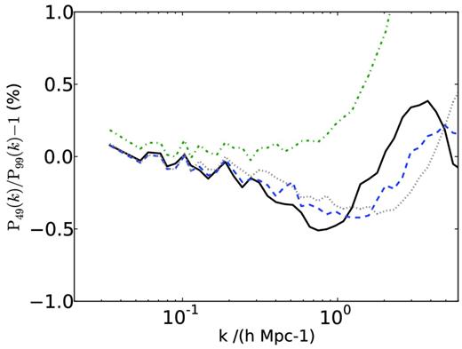
Change in the total matter power spectrum between S05 (initial redshift zi = 49) and S05IC (initial redshift zi = 99). Positive values correspond to more power in S05. Each line represents a different redshift: z = 9 (green dot–dashed), z = 3 (grey dotted), z = 1 (blue dashed) and z = 0 (black solid).
Fig. 3 shows the effect of changing the particle number, comparing S10 to S10P, which has eight times more particles. Changing the number of particles causes the sampling of initial structure to change slightly, introducing sample variance. To minimize this effect, we show the ratio of the suppression due to neutrinos for pairs of simulations with different particle numbers, that is, (PS10/PS00)/(PS10P/PS00P) − 1. Our results are converged at the 1 per cent level for k < 10 h−1 Mpc, and at the 0.2 per cent level for k < 1 h−1 Mpc. The effect of increasing particle resolution is to increase the overall growth of non-linear structure, and as a consequence to enhance the relative suppression due to massive neutrinos.
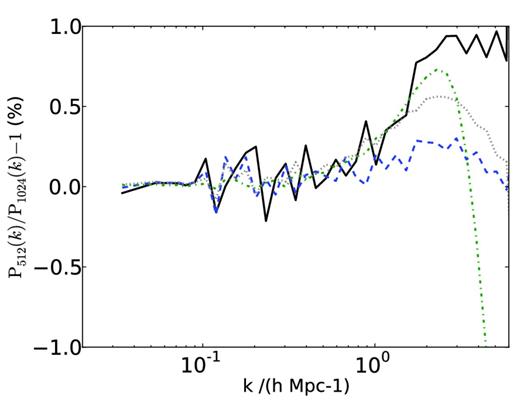
Effect of the number of CDM particles on the power suppression by neutrinos. What is plotted is the fractional difference between the ratio (PS10/PS00) (both using 5123 CDM particles) and the ratio (PS10P/PS00P) (both using 10243 CDM particles). Positive values correspond to a larger suppression of power in the 10243-particle simulation. Each line represents a different redshift: z = 9 (green dot–dashed), z = 3 (grey dotted), z = 1 (blue dashed) and z = 0 (black solid).
Total power spectra
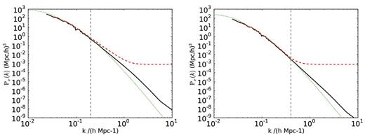
Fig. 4 shows the suppression in the total matter power spectrum, defined as the ratio between the total matter power spectrum including massive neutrinos with Mν = ∑mν = 0.3 eV and the matter power spectrum with massless neutrinos, but unchanged ΩM. The particle and Fourier neutrino simulation methods agree extremely well, and we see again the enhancement in the suppression due to the delayed onset of non-linear growth, as discussed in Bird et al. (2012).
The suppression in the total power spectrum at z = 0. Solid lines represent a 256 Mpc h−1 with our Fourier-based method (blue) and the particle method (red). The dashed line represents the prediction of linear theory. The spike at k ≈ 7 h Mpc−1 (corresponding to half the grid frequency) is a numerical artefact.
Fig. 5 shows the percentage difference in the total power spectrum between the particle and semilinear neutrino simulations, for redshifts between z = 3 and 0 and for a variety of neutrino masses. The agreement is extremely good in all cases. We show those scales where our simulation is resolved to less than 1 per cent; note that the difference between the two methods is generally smaller than the convergence error shown in Figs 2 and 3. The effect of non-linear growth in the neutrino component, neglected in our semilinear method, only begins to become important for Mν = 1.2 eV, at z < 1. Since neutrinos of this mass are already ruled out by current data, this is unlikely to be a practical limitation.
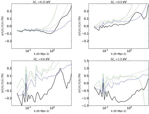
Percentage differences in the total matter power spectrum between the semilinear Fourier method and particles. ΔPt = PFourier − PParticle, so positive values correspond to more power in the Fourier method. The simulations used were S05 (top-left), S10 (top-right), S20 (bottom-left) and S40 (bottom-right). Each line represents a different redshift: z = 9 (green dot–dashed), z = 3 (grey dotted), z = 1 (blue dashed) and z = 0 (black solid).
One interesting feature is that on small scales we seem to see (slightly) more power in the Fourier method than the particle method, and the effect increases slightly at high redshift. This is not due to shot noise, which would lead to increased power in the particle method. This appears to be a convergence effect; as we have shown in Section 5.1, these scales are not converged to less than 1 per cent, and increasing the resolution of the simulation leads to a marginal increase of power on small scales. We therefore suspect that our semilinear method has an effective resolution slightly higher than the particle method, although if we computed the tree force for the neutrino particles, the situation would probably be reversed.
It is interesting to compare our results to those obtained using the original fully linear Fourier-space neutrino method of Brandbyge et al. (2008). Fig. 1 of that work is comparable to our Fig. 5. Our semilinear method agrees with the particle-based method slightly better in the linear regime. This is due to our derivation of the neutrino power spectrum from the CDM, which incorporates sample variance in the neutrino component in a way very similar to the particle method. In the non-linear regime, the agreement between the semilinear method and the particle method is significantly better than that between the fully linear and particle methods. The fully linear method shows differences from the particle method of >1 per cent for neutrinos with Mν = 0.6 eV, and has an error of about 5 per cent at 1.2 eV. We ran test simulations using the fully linear theory power spectrum, but with our improved model for the neutrino phase structure (i.e. assuming that the neutrinos are always in phase with the CDM rather than keeping their initial phases). The result was still in good agreement with Brandbyge et al. (2008), showing that the improved behaviour of the semilinear method in the non-linear regime does indeed result from accounting for the deeper non-linear potential wells sourcing the linear growth of neutrinos.
Bird et al. (2012), using the linear theory neutrino implementation of Viel et al. (2010), found somewhat larger differences between the linear and particle methods than Brandbyge et al. (2008). When preparing this work, we discovered that this was due to a slight inconsistency in the algorithm used; the Fourier-space neutrino implementation was altering the initial CDM transfer function to include neutrinos, adding the neutrino power when calculating long-range forces, but neglecting them when outputting the power spectrum. Once this was corrected, we obtain fully linear Fourier-space neutrino results in good agreement with those of Brandbyge et al. (2008).
Neutrino power spectra
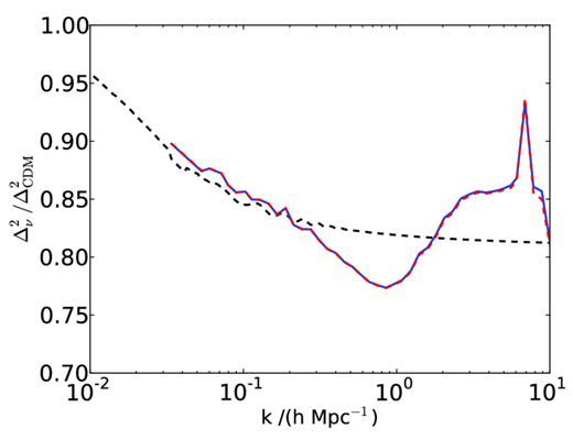
Fig. 6 shows the power spectra for the neutrino component at two different redshifts for the different methods. In the linear regime both codes agree well with linear theory. On non-linear scales our semilinear method shows additional power over the fully linear neutrino power spectrum. On all scales, PCDM ≫ Pν and k3Pν/(2π2) ≪ 1.
The power spectrum of the neutrino component at (left) z = 0 and (right) z = 1. Solid black represents the results of our semilinear Fourier-based method from simulation S10. Dashed red represents the particle method, from S10P, to obtain lower shot noise. Dotted green represents pure linear theory. The vertical dashed grey line represents the approximate non-linear scale for the dark matter.
At z = 0, the particle method produces additional power in the neutrino component. It begins to deviate from our semilinear Fourier-based method at k = knl, the non-linear scale for the dark matter. This first becomes apparent for z < 0.5, for all Mν ≥ 0.1 eV. We have checked that this area of the power spectrum is unchanged with a 5123-particle simulation, verifying that it is not being affected by shot noise. We ascribe this effect to non-linear growth in the neutrinos around the centres of clusters, as described in Ringwald & Wong (2004), Villaescusa-Navarro et al. (2011), and as we discussed in Section 2.4.
This does not appear to have any effect on the total matter power spectrum. Most of the effect of neutrinos on the total matter power spectrum comes from their time-integrated evolution; in particular, the size of the trough is due to their effect on the onset of non-linear growth. Since the highly non-linear effects on the neutrino power spectrum only take place at relatively late times, the impact on the total power spectrum is minimal. Moreover, on scales much smaller than the free-streaming scale, the main effect of including neutrinos is essentially to reduce the matter overdensity by a factor (1 − fν), while keeping the same background expansion rate (Lesgourgues & Pastor 2006). As long as |δν| < |δcdm|, the exact value of the neutrino overdensity does not matter very much. The same conclusion was reached by Shoji & Komatsu (2009), who compared their third-order perturbation theory calculations (for both CDM and neutrinos, the latter approximated as a perfect fluid with pressure) to a computation where CDM is treated to third order but neutrinos are computed to linear order (without accounting for non-linear growth of potentials), similar to the treatment of Saito et al. (2008). They found that although neutrino overdensities can be underestimated by order unity on non-linear scales, the total matter power spectrum is very accurately obtained, even with the simpler method.6
Finally, let us point out that for z > 0.5, subtracting the scale-free shot noise from Pν in the particle simulation produces very good agreement with the semilinear Fourier method, even at scales where the shot noise dominates. This is further evidence that neutrino shot noise is not having a strong dynamical effect, and is not causing spurious clustering.
Performance
Simulations S05–S20 were consistently faster when using our Fourier method. The speed increase was 13 per cent of the total walltime (which includes time spent reading and writing to disc). Note that the slowest single algorithm in gadget is the tree method for computing short-range forces, which is disabled for neutrinos even for our particle-based simulations, hence a large proportion of the execution time is independent of the method used to simulate neutrinos. More importantly, the total memory usage of gadget was 40 per cent smaller in the Fourier method than with particle neutrinos, essentially identical to the memory usage of a pure dark matter simulation. This is important because memory is often the limiting factor when performing large modern simulations.
The S10P simulation, which had eight times more dark matter particles than S10, took twelve times longer. This scaling is similar to that expected for a pure dark matter simulation, demonstrating that our neutrino method scales well. In fact, the only limit to scalability in the neutrino calculation is the need for interprocess communication when computing the power spectrum.
Overall, our Fourier method appears to have similar performance characteristics to a pure dark matter simulation, as should be expected; the time to compute the neutrino power spectrum is completely negligible compared to the N-body algorithms, and the most costly part of our Fourier algorithm is summing modes on the Fourier-transformed density grid to compute the power spectrum.
APPLICATIONS
Lyman α forest
The Lyman α forest is an indirect probe of the matter power spectrum at small, non-linear scales (k = 0.1-4 h− 1 Mpc), and at high redshift, z = 2-4. The power spectrum of the Lyman α flux measures the clustering of the absorption signal from neutral hydrogen in quasar spectra, and can be used to place constraints on the amplitude of primordial perturbations. When combined with constraints from large scales, this can lead to tight constraints on neutrino mass (Seljak 2000; Gratton et al. 2008; Viel et al. 2010). At these high redshifts, shot noise could be an issue for light neutrinos, so it is a natural place to apply our method. In addition, simulations with neutrino particles, dark matter and baryons can become unwieldy.
We used simulation F10BA to simulate the Lyman α forest at z = 2-4. Since the Lyman α forest is not the main focus of our paper, we shall not explain in detail our simulation methodology, and refer the interested reader to Viel et al. (2010). Our simulation calculates the clustering and ionization state of the gas at z = 2 using smooth particle hydrodynamics, together with radiative cooling and a reaction network which assumes optically thin gas in ionization equilibrium. We then simulate the flux in a set of 16 000 quasar spectra by calculating the absorption along random lines of sight. The averaged power spectrum of this flux is the observable quantity. Although constraints are available for k ≲ 4 h−1 Mpc, the Lyman α forest is also sensitive to the collapse scale of hydrogen absorbers k ∼ 60 h−1 Mpc, so very high resolution simulations are required. Fig. 7 shows the change in the flux power spectrum between our two methods; clearly, the differences are quite small. For simulations with the resolution of F10BA and mν = 0.1 eV, therefore, shot noise is not having a significant effect on the dynamics, even at z = 4, as also found by Viel et al. (2010). The total effect of neutrinos on the flux power is 5-10 per cent.
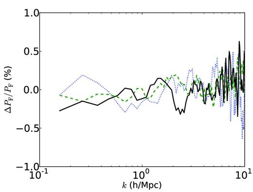
The change in the flux power spectrum between our Fourier method and the particle method, using simulation F10BA with mν = 0.1 eV. Positive values correspond to more power with the Fourier method. Each line represents a different redshift z = 4 (blue dotted), z = 3 (green dashed), and z = 2 (black solid). SDSS Lyman α data constrain the flux power spectrum for k ≲ 4 h−1 Mpc (McDonald et al. 2006).
Hierarchy
Achieving maximal accuracy for small neutrino masses requires us to account for the neutrino hierarchy. This is difficult in particle-based codes, as two neutrino species doubles the amount of memory required, but has been done (Wagner, Verde & Jimenez 2012). It is, however, essentially trivial using our method. We have performed two simulations (S03IH and S03NH) with a total neutrino mass of Mν = 0.1 eV using either the normal or inverted hierarchies, both to demonstrate the technique and to examine the effects of the hierarchy. For completeness, the masses of the three neutrino species were 0.022, 0.024 and 0.054 eV for S03NH, and 0, 0.049 and 0.051 eV for S03IH. Our results are shown in Fig. 8, together with the prediction of linear theory. The linear theory change due to the hierarchy is quite small (below our convergence error). Furthermore, the effect in linear theory is mostly due to the change in background evolution caused by one of the possible hierarchies having one massless species. As shown in fig. 16 of Lesgourgues & Pastor (2006), the difference between the hierarchies when all three neutrino species are massive in both cases is much less. Although differences in our cosmological parameters mean that the linear effect is smaller than that found by Wagner et al. (2012), we still find, as they did, an enhancement at non-linear scales, analogous to the enhancement for the total neutrino effect shown in Fig. 4. Determining the hierarchy separately from the total neutrino mass from an effect this subtle is likely to prove challenging. However, obtaining robust constraints with Mν ≲ 0.1 eV will require accounting for the mass splitting.
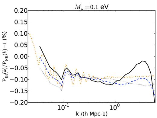
The difference in the total matter power spectrum between the inverted and normal neutrino hierarchies. Negative values correspond to more power in the normal scenario. Each line represents a different redshift: z = 3 (grey dotted), z = 1 (blue dashed) and z = 0 (black solid). The orange dot–dashed line represents the linear prediction at z = 0.
21 cm forest
Observations of the spin-flip transition of neutral hydrogen in the 21 cm forest have the potential to probe structure growth at z ∼ 20 (McQuinn et al. 2006). Structure formation at these redshifts is sensitive to the non-linear growth of the first, small haloes. No one has yet examined the impact of neutrinos on the 21 cm forest, and performing the requisite simulations is beyond the scope of this paper. However, our code would be ideal for such a study. Haloes at these redshifts are not yet sufficiently massive for our method to break down in their central region, so one could probe arbitrarily small scales. Furthermore, shot noise would be a severe issue for the particle method at these redshifts.
DISCUSSION AND CONCLUSIONS
We have presented a new semilinear method for simulating the effects of massive neutrinos on cosmic structure, taking advantage of the hierarchy between the neutrino free-streaming scale and the non-linear scale, kfs < knl for currently allowed neutrino masses. The power spectrum of the neutrino component is calculated using perturbation theory, and added to the CDM in Fourier space, as in Brandbyge et al. (2008). However, we improve upon their method by sourcing neutrino perturbations using the gravitational potential obtained from the full non-linear dark matter overdensity rather than from the dark matter power predicted by linear theory. We evolve the CDM, baryons and neutrinos simultaneously and self-consistently.
For observationally relevant neutrino masses, our method gives results for the non-linear power spectrum essentially identical to a fully converged neutrino particle treatment, a significant increase in accuracy over fully linear Fourier-space neutrinos. Our method also has several advantages over a particle treatment; it is faster, uses significantly less memory and does not suffer from shot noise in the neutrino component. Furthermore, it allows for an easy inclusion of the correct background evolution with relativistic corrections, and makes inclusion of the neutrino hierarchy trivial. These properties make it especially suitable for simulating neutrinos at the low end of the currently allowed mass range.
Our treatment is not strictly valid in the inner regions of very massive haloes, where the escape velocity might be larger than the thermal velocity of neutrinos, which may be captured and cluster non-linearly. Accurately describing the distribution of neutrinos in these haloes requires treating them as N-body particles. Because of this effect, we do not accurately recover the non-linear neutrino power spectrum at redshifts z < 0.5. However, this does not affect the total matter power spectrum, because on the one hand most of the neutrino effect is imprinted at earlier times, where our method is extremely accurate, and on the other hand, even with an enhanced clustering due to non-linear growth, neutrino overdensities are very subdominant compared to those of the CDM.
While we have focused on neutrinos, our treatment can also be easily applied to any HDM particle whose characteristic velocity is larger than (or at least of the order of) the escape velocity of massive clusters, and whose free-streaming length today is larger than the non-linear scale. There are many applications of our method beyond the non-linear matter power spectrum; we have briefly discussed the Lyman α and 21 cm forests. It allows the inclusion of neutrinos in an N-body simulation at minimal cost and effort, and should thus be useful for any problem in non-linear structure formation.
We thank Volker Springel for allowing one of us (SB) to use the code gadget-3, Matteo Viel for useful discussions and Daniel Grin for enlightening conversations on various aspects of this work. We are grateful to Anthony Challinor, Julien Lesgourgues and Eiichiro Komatsu for providing detailed comments on the draft of this paper, and acknowledge conversations with Matias Zaldarriaga, Scott Tremaine, Marilena LoVerde and Tobias Heinemann. The authors are supported by the National Science Foundation grants AST-080744 (for YA) and AST-0907969 (for SB).
NOVA proposal: http://www-nova.fnal.gov/.
The shot noise issue arises for neutrinos for two reasons. First, their large random velocities effectively randomly distribute them over the box, which leads to a Poisson spectrum |$P(k) = 1/\overline{n}$| at all scales. Secondly, their intrinsic clustering is very small on small scales. At large enough redshifts and for small enough scales, the true power may be completely swamped by the Poisson noise.
Note that consistently accounting for relativistic corrections in the evolution of neutrinos would also require accounting for CMB inhomogeneities sourcing the gravitational potentials; these are always (rightfully so) neglected in N-body simulations.
Interestingly, for a relativistic Fermi–Dirac distribution, the small-scale overdensity obtained from the linearized version of equation (49) is larger than the one obtained from the full non-linear equation.
Our initial conditions generator is freely available at http://github.com/sbird/S-GenIC
REFERENCES
APPENDIX A: ANALYTIC APPROXIMATION FOR LINEAR HDM CLUSTERING
APPENDIX B: ACCURACY OF THE ITERATIVE SOLUTION FOR THE NEUTRINO POWER SPECTRUM
APPENDIX C: FITTING FUNCTION FOR |$\mathcal {I}(X)$|
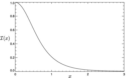
Function |$\mathcal {I}(x)$| that determines the damping of perturbations due to free-streaming of neutrinos (equation 38 with x = XTν, 0).
