


Abstract
We describe a methodology to accurately compute halo mass functions, progenitor mass functions, merger rates and merger trees in non-cold dark matter universes using a self-consistent treatment of the generalized extended Press–Schechter formalism. Our approach permits rapid exploration of the subhalo population of galactic haloes in dark matter models with a variety of different particle properties or universes with rolling, truncated or more complicated power spectra. We make detailed comparisons of analytically derived mass functions and merger histories with recent warm dark matter cosmological N-body simulations, and find excellent agreement. We show that once the accretion of smoothly distributed matter is accounted for, coarse-grained statistics such as the mass accretion history of haloes can be almost indistinguishable between cold and warm dark matter cases. However, the halo mass function and progenitor mass functions differ significantly, with the warm dark matter cases being strongly suppressed below the free-streaming scale of the dark matter. We demonstrate the importance of using the correct solution for the excursion set barrier first-crossing distribution in warm dark matter – if the solution for a flat barrier is used instead, the truncation of the halo mass function is much slower, leading to an overestimate of the number of low-mass haloes.
1 INTRODUCTION
The cold dark matter (CDM) paradigm (Peebles 1982) works extremely well on large scales (Seljak et al. 2005; Percival et al. 2007; Ferramacho, Blanchard & Zolnierowski 2009; Sánchez et al. 2009; Komatsu et al. 2011), but there remains the possibility of deviations from the CDM expectations on small scales – arising notably from the issue of cores versus cusps and the inner slope of dark matter density profiles (Salucci 2001; Donato, Gentile & Salucci 2004; Donato et al. 2009; Newman et al. 2009, 2011; de Blok 2010; Kuzio de Naray & Kaufmann 2011; Kuzio de Naray & Spekkens 2011; Salucci et al. 2012; Wolf & Bullock 2012) and the apparent paucity of bright satellites around the Milky Way (Boylan-Kolchin, Bullock & Kaplinghat 2011, 2012; although see Wang et al. 2012). Several extensions to dark matter phenomenology (Markevitch et al. 2004; Ahn & Shapiro 2005; Boehm & Schaeffer 2005; Miranda & Macciò 2007; Randall et al. 2008; Boyarsky et al. 2009; Lovell et al. 2012) and several different particle physics candidates for dark matter (Raffelt 1990; Turner 1990; Jungman, Kamionkowski & Griest 1996; Hogan & Dalcanton 2000; Spergel & Steinhardt 2000; Abazajian, Fuller & Patel 2001; Cheng, Feng & Matchev 2002; Feng, Rajaraman & Takayama 2003; Sigurdson & Kamionkowski 2004; Hubisz & Meade 2005; Feng et al. 2009) have been put forward to explain these deviations, although it remains unclear if any of these proposals is able to fully explain observed phenomena (Kuzio de Naray et al. 2010) or if they are even necessary, with the observed phenomena simply being a consequence of galaxy formation physics in a CDM universe (Benson et al. 2002b; Libeskind et al. 2007; Li et al. 2009; Stringer, Cole & Frenk 2010; Font et al. 2011; Oh et al. 2011; Governato et al. 2012; Kuhlen et al. 2012; Pfrommer, Chang & Broderick 2012; Pontzen & Governato 2012; Starkenburg et al. 2012; Vera-Ciro et al. 2012). A variety of experimental measurements may be sensitive to the small-scale structure of dark matter haloes (Simon et al. 2005; Viel et al. 2008). The most promising are future lensing experiments, which have the potential to strongly constrain dark matter particle phenomenology (Keeton & Moustakas 2009; Vegetti & Koopmans 2009a,b; Vegetti, Czoske & Koopmans 2010a; Vegetti et al. 2010b, 2012). A variety of previous works have shown that the subhalo mass function should depend sensitively on the dark matter physics and the shape of the power spectrum. To maximize the scientific return of future experiments therefore requires the ability to accurately and rapidly predict the distribution of dark matter substructure as a function of dark matter particle thermal or interaction properties, for arbitrary power spectra.
In this work, we develop techniques to follow the growth of non-linear structure in non-CDM universes using a fully consistent treatment of the extended Press–Schechter formalism. We demonstrate the performance of these techniques by applying them to a representative case of warm dark matter (WDM), which has the advantage of several pre-existing N-body simulations which we utilize to test the accuracy of our methods. WDM particles1 are lighter than their CDM counterparts, allowing them to remain relativistic for longer in the early universe and to retain a non-negligible thermal velocity dispersion. This velocity dispersion allows them to free-stream out of density perturbations and so suppresses the growth of structure on small scales (Bond & Szalay 1983; Bardeen et al. 1986). While mass functions have been previously considered in this case (Barkana, Haiman & Ostriker 2001), we go one step further and develop methods to compute conditional mass functions and halo merger rates, and use these to construct merger trees in WDM universes. These merger trees are a key ingredient required to predict the distribution of substructure masses, positions and internal structure as is necessary to make detailed predictions for future lensing experiments.
The remainder of this paper is organized as follows. In Section 2, we describe the changes that we introduce to the extended Press–Schechter formalism to make it applicable to the case of non-CDM scenarios (including some specifics for the WDM case). In Section 3, we apply these methods to the case of WDM, first comparing their predictions to the available data from N-body simulations, then exploring the limitations of ignoring the effects of WDM velocity dispersion and presenting a comparison of key results between WDM and CDM. Finally, in Section 4, we discuss the consequences of this work and present our conclusions.
We also include two appendices. Appendix A gives a detailed derivation of our numerical procedure for solving the excursion set first-crossing problem for arbitrary barriers. Appendix B explores the numerical accuracy and robustness of the methods developed in this work.
When comparing our analytic theory with results from N-body simulations we will adopt the same cosmological parameters and dark matter particle properties as were used for the simulation. These values will be listed where relevant. For the rest of this work, specifically in Sections 2, 3.23.3 and Appendix B we adopt a canonical cosmological model with ΩM = 0.2725, |$\Omega _\Lambda =0.7275$|, Ωb = 0.0455 and H0 = 70.2 km s−1 Mpc−1 (Komatsu et al. 2011) and a canonical WDM particle of mass, mX = 1.5 keV and effective number of degrees of freedom gX = 1.5 (the expected value for a fermionic spin-|$\frac{1}{2}$| particle).
2 METHODS
Our approach makes use of the Press–Schechter formalism (Press & Schechter 1974; Bond et al. 1991; Bower 1991; Lacey & Cole 1993) which, after substantial development and tuning against N-body simulations, has proven to be extremely valuable in understanding the statistical properties of dark matter halo growth in CDM universes. The Press–Schechter formalism in its modern form is expressed in terms of excursion sets – the set of all possible random walks in density at a point as the density field is smoothed on ever smaller scales. Halo formation corresponds to a random walk making its first crossing of a barrier. The height of that barrier is determined from models of the non-linear collapse of simple overdensities.
The Press–Schechter algorithm requires three ingredients: (1) the power spectrum of fluctuations in the density field (characterized by σ(M), the fractional root variance in the linear theory density field at z = 0); (2) the critical threshold in linear theory corresponding to the gravitational collapse of a density perturbation δc; and (3) a solution for the statistics of excursion sets to cross this threshold. We will address each of these three ingredients below.
2.1 Power spectrum
2.1.1 Window function
However, in the case of power spectra with a small-scale cutoff, such as those of WDM models and many other non-CDM candidates, the situation is very different. With a top-hat window function, σ(M) continues to increase with decreasing filter mass even for masses well below the cutoff scale. This happens because although there are no new intrinsic small-scale modes entering the filter, the longer wavelength modes are getting reweighted as the mass scale of the filter increases. In contrast, with a sharp k filter, σ(M) increases monotonically up to the cutoff scale and then becomes constant with the transition being determined by the abruptness of the cutoff in the input WDM power spectrum. Since the Press–Schechter mass functions depend directly on σ(M), including a direct dependence on the logarithmic slope of σ(M), its predictions for the case of WDM are sensitive to this choice. Hence, for non-CDM models, it is important to revisit the issue of filter choice and one would expect that the conventional top-hat choice will lead to an overestimate of the number of low-mass haloes [an effect apparent in the works of Barkana et al. (2001) and Menci, Fiore & Lamastra (2012)].
We begin by adopting the sharp k-space window function of equation (3) when working with truncated power spectra, such that the contribution from long-wavelength modes remains constant. In the case of a top-hat real-space window function, there is a natural relation between the top-hat radius and the smoothing mass scale, as given by equation (5). In the case of a sharp k-space window function, the choice of ks(M) is less clear. Lacey & Cole (1993) suggest choosing |$\stackrel{\sim }{W}\!\!(r=0)=1$| (where |$\stackrel{\sim }{W}\!\!(r)$| is the Fourier transform of the window function) and then choosing ks(M) such that the integral of the mean density, |$\bar{\rho }$|, under |$\stackrel{\sim }{W}\!\!(r)$| equals the required smoothing mass, M. However, as noted by Lacey & Cole (1993), this choice for ks(M) lacks any strong physical motivation.
We note that fixing the ks(M) relation in this way introduces a free parameter, a, into our method and introduces a dependence on the N-body simulation to which we will compare our results in Section 3.1.1. However, given that the CDM linear power spectrum is close to a power law on the scales that will be of interest for WDM models and that the modification to the transfer function due to WDM scales simply with the mass of the dark matter particle, we expect that the same choice of a should be valid for all WDM particle masses of interest.
Fig. 1 shows the resulting root variance in the density field (smoothed using a top-hat filter in real space) as a function of mass enclosed within the filter for both WDM and CDM models. As expected, σ(M) in our WDM model is suppressed below the CDM value for M ≲ Ms.
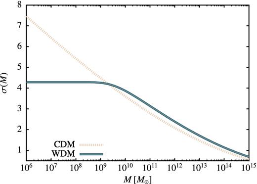
The fractional root variance of the mass density field as a function of the mean mass contained within that filter. Both CDM and our canonical WDM cases are shown. A top-hat real-space window function is used for the CDM, while a sharp k-space filter is used for WDM. The WDM case is suppressed below the CDM value for M ≲ Ms.
2.2 Critical overdensity for collapse (excursion set barrier)
The Press–Schechter algorithm as formulated by Bond et al. (1991) associates the collapse of a dark matter halo with a random walk in δ(M) making its first crossing of some barrier, B(S). This barrier is usually associated with the critical linear theory overdensity for collapse of spherical top-hat perturbations (although see Section 2.2.1 for a refinement of this assumption). In the CDM case, that critical overdensity is independent of mass scale (since there are no preferred scales in the problem). In the non-CDM case, this is no longer true. For example, with WDM we expect collapse to become significantly more difficult on small scales, where the WDM particles can stream out of collapsing overdensities due to their non-zero random velocities. Barkana et al. (2001) addressed the question of collapse thresholds in WDM universes by performing a set of 1D hydrodynamical simulations, in which pressure acted as a proxy for the velocity dispersion of WDM particles. They find that the growth of collapsing overdensities is suppressed below a characteristic mass scale – i.e. the threshold for collapse increases rapidly with decreasing mass below the characteristic mass scale.
The ratio of the resulting critical overdensity to the CDM value with masses scaled to MJ is shown in Fig. 2. For M/MJ ≲ 1, the critical overdensity for collapse in WDM universes is much higher than in CDM as a result of the non-zero velocity dispersion of WDM particles. A small-scale perturbation must have a much larger density for its self-gravity to overcome this velocity dispersion and cause collapse.
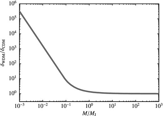
The critical linear theory overdensity for the collapse of a spherical top-hat density perturbation in a WDM universe normalized to that in a CDM universe as a function of halo mass, M (expressed in units of the effective Jeans mass of the WDM, MJ). For M/MJ ≫ 1 the WDM and CDM cases coincide, but for M/MJ ≲ 1 WDM requires a much larger overdensity to undergo gravitational collapse.
We emphasize that the calculations of Barkana et al. (2001) are approximate as they are based on a hydrodynamical approximation which will not fully capture the collisionless dynamics of WDM. We expect that the approximation made by Barkana et al. (2001) could lead to a small (order unity) difference in the characteristic mass scale for suppression of overdensity collapse (e.g. in a similar way that the Toomre stability threshold for collisionless stars and gas differ by a factor of π/3.36). There could plausibly be differences in detail in the shape of the collapse threshold as a function of mass, but we are unable to speculate what form those might take. A more realistic calculation using a Boltzmann solver should be carried out to improve upon these results and explore the dependence on cosmological parameters.
2.2.1 Barrier remapping
2.2.2 Barrier scaling
As noted in Section 2.1.1 our choice of normalization for the window function used to derived σ(M) from P(k) results in σ(M) for the WDM case lying above the CDM case for large masses. This will change the halo mass function for high-mass haloes – something which is not expected (i.e. WDM should behave just like CDM on sufficiently large scales). Therefore, we introduce a global rescaling of the barrier (applied after the remapping described in Section 2.2.1 – an important point since that remapping is non-linear), multiplying it by a factor of 1.197. This value is chosen to counteract the higher σ(M) on large scales8 and ensure that the mass function of high-mass haloes remains unchanged (see Section 2.1.1 for discussion of this point). This rescaling of the barrier is always included, both when computing halo mass functions and when computing halo merger rates. We note that this factor is very insensitive to cosmological parameters and σ8 as it depends only upon the shape of the power spectrum (not the normalization). For example, if we compute the appropriate rescaling factor for Wilkinson Microwave Anisotropy Probe 1 (WMAP1) cosmological parameters (rather than the WMAP7 cosmological parameters used throughout this work), we find that the factor changes by <0.1 per cent (despite there being a difference of 11 per cent in σ8).
The resulting excursion set barriers for both CDM and our canonical WDM models (including both remapping and subsequent rescaling) are shown in Fig. 3. For large masses the two are offset by a factor of 1.197, but the WDM barrier becomes very large for M ≪ Ms due to the velocity dispersion of the WDM particles.
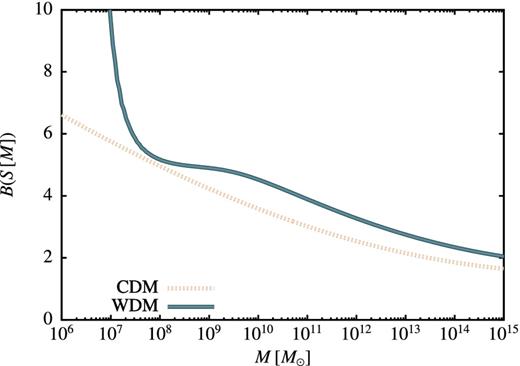
The barrier for excursion sets in both the CDM and our canonical WDM cases. For large masses the two are offset by the constant factor of 1.197 which accounts for the difference in definition (top-hat real-space versus sharp k-space window functions) of σ2(M) in the two cases, but the WDM barrier becomes very large for M ≪ Ms. Below M ∼ Ms the WDM barrier rises rapidly due to the velocity dispersion of WDM particles.
2.3 Excursion sets/barrier crossing
Given a barrier, B(S), and the variance of the density field, S(M), the Press–Schechter algorithm proceeds by following random walks in δ(S) beginning from (δ, S) = (0, 0). When a given random walk first crosses the barrier at some variance S, it is assumed that the point in question has collapsed into a halo of mass M(S). The fraction of random walks crossing between S and S + dS, f(S)dS, corresponds to the fraction of mass in the universe in haloes of mass M to M + dM.
2.4 Merger rates and progenitor mass functions
The original Press–Schechter algorithm has been extended to compute conditional mass functions (i.e. the mass function of haloes which will all belong to a single halo of larger mass at some later time; Lacey & Cole 1993). Further, the form of the conditional mass function in the limit of small timestep has been used to estimate merger rates of dark matter haloes and so to construct merger trees (Cole et al. 2000). We therefore wish to compute the conditional mass function in the WDM case, specifically in the limit of small δt. In the excursion set approach, the conditional mass function is found by simply solving the first-crossing problem beginning from the (δ, S) of the parent halo and using a barrier corresponding to an earlier time. This is equivalent to solving the original first-crossing problem with a modified barrier B′(S′, t1, t0) = B(S′ + S, t1) − B(S, t0).
To compute merger rates we therefore solve the first-crossing problem using our numerical method but with an effective barrier B′(S′, t1, t0). We choose t1 = (1 − ϵ)t0 where ϵ ≪ 1. The rate of crossing this effective barrier can then be estimated as f(S)/ϵt0. We will explore the sensitivity of our results to the value of the numerical parameter ϵ.
When solving for halo merger rates we do not include any remapping of the barrier function (as discussed in Section 2.2.1). The remapping function was chosen to result in good agreement between the Press–Schechter halo mass function and that measured in the Millennium N-body simulations (Springel et al. 2005). However, our merger rates will be used in merger tree construction algorithms which, in the CDM case, have been developed to work with a barrier with no remapping, but with their own empirical modification of merger rates designed to match progenitor mass functions found in N-body simulations (see Section 2.5 for further discussion). Scaling of the barrier (see Section 2.2.2) is included however.
2.5 Merger tree construction
We retain the same empirical modification in this work since it should remain valid for WDM in the limit of high-mass haloes. For masses comparable to and below Ms, this empirical modification may no longer be accurate. Our justification for retaining this empirical modification is the good agreement achieved with progenitor mass functions from N-body simulations of WDM as will be shown in Section 3.1.
A timestep is then chosen that is sufficiently small such that the probability of multiple branchings is small and the fractional change in mass due to subresolution accretion is small. This timestep is then taken, branching if a random deviate lies below the branching probability, and with mass removed at the rate of subresolution accretion. If branching does occur, the mass of one of the branched haloes is selected at random from the distribution d2f/ dωdM′ and the other is chosen to ensure mass conservation.
2.5.1 Smooth accretion
3 RESULTS FOR WARM DARK MATTER
The methods described in Section 2 have been implemented within the open source semi-analytic galaxy formation code, galacticus (Benson 2012). All results presented in this section were generated using galacticus v0.9.1 r903. Control files and scripts to generate all results presented in this paper using galacticus can be found at http://users.obs.carnegiescience.edu/abenson/galacticus/parameters/dmMergingBeyondCDM1.tar.bz2.
We consider three different WDM particle masses. In Section 3.1.1 we use mX = 0.25 keV to match the N-body simulations of Schneider et al. (2012), in Section 3.1.2 we use mX = 2.2 keV to match the Aquarius WDM counterpart simulations (described below) and in Section 3.3 we use mX = 1.5 keV in comparisons of WDM and CDM. For reference, Fig. 4 shows the halo mass function in these three cases, illustrating the expected increase in the cutoff mass, ms, as the WDM particle mass is decreased.
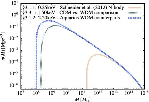
Dark matter halo mass functions, computed using the methods described in Section 2, for the three different WDM particle masses considered in this work. The labels give the particle mass and the section of this work in which that mass is used.
3.1 Comparison with N-body simulations
3.1.1 Halo mass function
N-body simulations should, in principle, provide an accurate determination of the dark matter halo mass function in WDM cosmologies, provided that initial conditions are constructed carefully. The points in Fig. 5 show the mass function measured in an N-body simulation of 0.25 keV WDM carried out by Schneider et al. (2012). The upturn below 2 × 10¹¹ M⊙ is a numerical artefact, arising from the fragmentation of filaments due to particle discreteness (Wang & White 2007). This is a challenging problem for N-body simulations of WDM as the mass scale at which the upturn appears decreases only as N−1/3 (where N is the particle number).
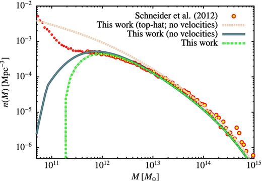
The dark matter halo mass function for WDM in the case of a 0.25 keV particle. The points show the results of an N-body simulation of WDM from Schneider et al. (2012) (small points are used to indicate the region in which the N-body simulation results are unreliable as a result of being dominated by haloes formed through artificial fragmentation), while the line shows the result from this work with dark matter properties and cosmological parameters matched to those used by Schneider et al. (2012). Note that the upturn in the N-body mass function below 2 × 10¹¹ M⊙ arises to artificial fragmentation of filaments (see Wang & White 2007).
The solid line in Fig. 5 shows the mass function predicted by our calculation using the same cosmological and WDM particle parameters as in Schneider et al. (2012). Schneider et al. (2012) identified haloes using a friends-of-friends (FOF) algorithm with a linking length of b = 0.2, corresponding approximately to density contrasts of 200. In our model, the relevant density contrasts are those arising from the spherical top-hat collapse model (e.g. Percival 2005). We correct the masses reported by Schneider et al. (2012) for this difference by assuming that the haloes have NFW density profiles (Navarro, Frenk & White 1997) with concentrations given by the CDM results of Gao et al. (2008) modified by the WDM-to-CDM conversion factor reported by Schneider et al. (2012). Additionally, Schneider et al. (2012) do not include any velocity dispersion of dark matter particles in their initial conditions and so the fairest comparison is the one in which we do not modify the critical overdensity for collapse as described in Section 2.2.
Results of three different calculations from this work are shown in Fig. 5. Going from top to bottom, the first two lines do not include the effects of velocity dispersion (consistent with Schneider et al. 2012). The first line corresponds to a case where we use a top-hat real-space window function to determine σ(M). It can be seen that this curve, while in good agreement with the N-body results for high masses, does not produce sufficient suppression of the mass function at lower masses – a similar discrepancy was seen by Barkana et al. (2001) when comparing their Press–Schechter-based model for WDM halo formation to the N-body simulations of Bode et al. (2001). The second line (blue) switches to using a sharp k-space window function as described in Section 2.1.1. For high-mass haloes, this results in only a small change in the mass function compared to the CDM case due to the difference in S(M) when computed with sharp k-space and top-hat window functions (even after scaling the barrier height to compensate for this difference as much as possible; see Section 2.2.2),10 but also results in an excellent match to the suppression of the abundance of low-mass haloes, indicating that the discrepancies found in previous works were due to the artificial increasing in σ(M) below the cutoff which arises when a top-hat real-space filter is used. At the lowest masses the suppression of the mass function is masked in the N-body simulation as it is masked by the upturn due to artificial fragmentation of filaments. Finally, the green line adds in the effects of velocity dispersion (which are not included in the N-body simulation), illustrating the importance of this effect to accurately model the suppression of the lowest mass haloes.
3.1.2 Progenitor mass functions/merger rates
A set of WDM Milky Way mass haloes have been simulated and analysed in Lovell et al. (in preparation). The haloes they simulated are WDM counterparts of the Aquarius CDM haloes presented in Springel et al. (2008), and so have masses of the order of |$10^{12}\,\text{M}_{\odot }$| – we will therefore refer to them as ‘Milky Way-mass WDM simulations’. Here we make use of a set of four (A–D) haloes simulated with approximately 40 million particles within their virial radii (resolution level 3 in the notation of the Aquarius project). One of the haloes (A) has also been run at higher (level 2) resolution, and we have used this to verify that the progenitor mass functions that we show in Fig. 6 have accurately converged over the range of masses plotted. The cosmological parameters for this set of simulations were chosen to match the WMAP7 results of Komatsu et al. (2011); however, the CDM power spectrum was modified using the prescription of Bode et al. (2001) for WDM as given in our equation (1) with a smoothing scale of λs = 78.4 kpc, corresponding to an approximately 2.2 keV thermal WDM particle. In each of the simulations, haloes and subhaloes were identified at each of the 128 output times using the FOF (Davis et al. 1985) and subfind (Springel et al. 2001) algorithms, respectively. Merger trees of subhaloes were constructed by identifying the descendant of each subhalo and halo merger trees built from the subhalo membership of each halo as described in Jiang et al. (in preparation) and Merson et al. (2012). These halo merger trees can be thought of as FOF halo merger trees that have been cleaned up to avoid problems that occur when FOF haloes are essentially composed of two distinct haloes linked by a low-density bridge.
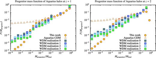
Progenitor mass functions of four realizations of the Milky Way-mass WDM dark matter haloes at z = 1 and 2 (squares) compared with the predictions of this work (circles). For reference, the corresponding progenitor mass functions from one realization of the Aquarius CDM simulations are shown as triangles. Each panel shows the fraction of the halo mass contributed by progenitors in each mass bin. Masses are shown as a fraction of the final halo mass.
The issue of spurious haloes formed by the fragmentation of filaments due to numerical noise (Wang & White 2007) is investigated in Lovell et al. (in preparation). They find that most of such (sub)haloes can be identified by looking at the shape in the initial conditions of the region from which their particles originated. The spurious (sub)haloes typically originate from very flattened configurations. Lovell et al. determine a threshold on the axis ratio, c/a, of the inertia tensor of the initial particle distribution such that for a CDM simulation 99 per cent of haloes pass this cut, while in a WDM simulation most of the spurious haloes are excluded. Here we use this criterion to exclude complete subhalo branches from the N-body merger trees. In these N-body merger trees, the same subhalo is identified at subsequent epochs by tracing the fate of a fraction of its most bound particles. In this way we can identify the point at which a halo dissolves as a result of disruption within a larger (sub)halo and form a branch consisting of its main progenitor at all earlier times. We discard such a branch if at the point at which this subhalo had half its maximum mass, the subhalo fails the cut on the initial axis ratio.
Fig. 6 compares the progenitor mass functions measured from a large number of merger tree realizations generated using the techniques described in this work (circles) compared with the progenitor mass functions measured from four Milky Way-mass WDM simulation haloes (squares). For reference, the equivalent CDM progenitor mass function from a single realization of the Aquarius simulations is shown (triangles). Given the halo-to-halo scatter, there is good agreement down to Mprogenitor/Mfinal ≈ 10−4. Below this, the abundance of progenitors in the WDM N-body simulations exceeds that predicted by our techniques. At these mass scales, the artificial halo rejection algorithm reduces the number of progenitors by over an order of magnitude. This excess of low-mass progenitor haloes is consistent with the failure rate for the artificial halo rejection algorithm of slightly less than 10 per cent. We cannot rule out such a failure rate in the algorithm and so the true progenitor mass function could decline much more rapidly. The progenitor mass functions from our analytic calculations decline rapidly as they approach Mprogenitor/Mfinal ≈ 10−4, but then transition to a slower, power-law decline at lower masses. As will be discussed in Section 3.3.3, this appears to be due to the finite difference approximation used to compute merger rates (see Section 2.4) and so can be suppressed as necessary by lowering the value of ϵ.
In the CDM case, the mass function (expressed in this way) levels off to be almost constant below Mprogenitor/Mfinal ∼ 10−3. In our calculation, which tracks the CDM case extremely well at high masses, this flattening begins (for Mprogenitor/Mfinal ≳ 10−3) but is then interrupted by the cutoff due to WDM physics. The result is a ‘bump’ feature. The presence of such a bump is less clear in the WDM N-body progenitor mass functions (although there is a hint of it in the z = 1 results) due to the noisiness of those results. This feature may have interesting implications for the expected number of surviving dwarf scale subhaloes, and so represents an interesting avenue for future investigation.
3.2 Limitations of only modifying power spectrum
Having demonstrated that our model is consistent with the available N-body simulation we now consider the effects of treating WDM incorrectly or incompletely in the extended Press–Schechter approach, as has previously happened in the literature (Menci et al. 2012). Fig. 7 shows a series of results for the halo mass function for 1.5 keV WDM. For reference, line 1 shows the mass function for CDM derived assuming a mass-independent critical overdensity. Line 2 switches to using the WDM power spectrum, but retains the CDM mass-independent critical overdensity. There is a clear suppression of the mass function below Ms. Line 3 now uses the WDM power spectrum and adds mass dependence to the critical overdensity, but still uses the barrier crossing solution for a linear barrier11 given in equation (B1). The suppression of the mass function is almost unchanged compared to the previous case where we used the CDM critical overdensity. Finally, line 4 shows the result of switching to using the correct, numerically determined, functional form for f(S). The mass scale of the cutoff undergoes a dramatic shift of almost an order of magnitude to higher mass compared to the previous case. The reason for this is simple to understand. When using the WDM B(S) in flinear(S) we are implicitly assuming that the barrier is flat at the same value of B(S) at all smaller S [this being the assumption used to derive flinear(S)]. This gives a certain crossing probability. When we numerically determine fcorrect(S), the full S dependence of the barrier is taken into account. In the first case, a random walk crossing B(S) at S must have remained below B(S) for all S′ < S, while in the second case it must have remained below B(S′) for all S′ < S. Since B(S′) < B(S) for all S′ < S, this second condition is much more stringent, and so far fewer random walks will satisfy it. Thus, the crossing probability, and so the mass function, will be more strongly suppressed. This illustrates the importance of correctly solving the barrier crossing problem for WDM calculations.
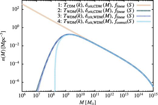
The dark matter halo mass function for CDM (line 1) and for various approximations to the 1.5 keV WDM solution. Line 2 shows the result of using the WDM transfer function, but retaining the CDM mass-independent critical overdensity and the functional form of f(S) appropriate to a linear barrier, flinear(S). Line 3 improves on this approximation by using the correct mass-dependent WDM critical overdensity, but still uses flinear(S). Finally, line 4 shows the result of using the correct functional form of f(S) for the WDM barrier. Note that, for large halo masses, all lines coincide precisely and so are hidden beneath line 4.
3.3 Warm versus cold dark matter
In the following we compare example results for CDM and 1.5 keV WDM cases. This WDM particle mass differs from those used in previous sections (where the choice was constrained to match those assumed in different N-body simulations). In all cases, we use the correct f(S) (determined numerically for the WDM case) and include remapping of the barrier for calculations of first-crossing probabilities and mass functions.
3.3.1 Mass functions
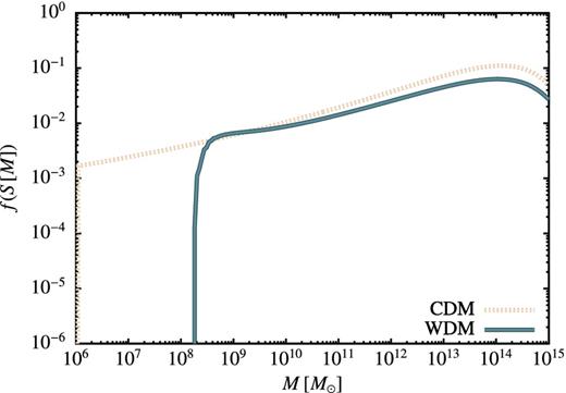
The first-crossing probability, f(S), is shown as a function of mass, M, for both CDM and WDM cases for z = 0.
Below around Ms the WDM first-crossing probability is suppressed due to the rapidly rising barrier B(S). (There is a small region where the WDM f(S) exceeds that of CDM due to differences in the mapping from M to S in the two cases.)
These first-crossing distributions translate directly into halo mass functions, as shown by lines 1 and 4 of Fig. 7. As expected, the suppression in f(S) in WDM translates into a strong suppression in the mass function below around Ms. At larger masses, the two are indistinguishable.
3.3.2 Merger rates
Fig. 9 shows the rate of first crossing for CDM and WDM barriers for a 1012 M⊙ halo at z = 0. The two lines almost coincide at high mass, although the WDM line lies slightly below the CDM line.12 The merger rate in the WDM case is strongly suppressed below around Ms due to the lack of halo in that mass range. The slight enhancement in the rate of first crossing in WDM compared to CDM just above Ms is due to the different mapping between mass and variance in the two cases.
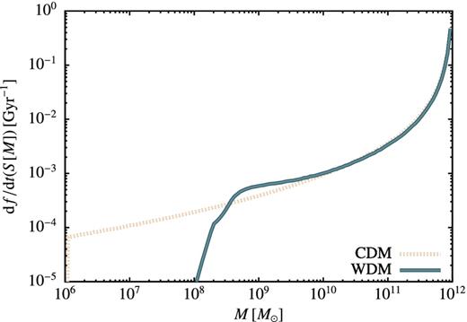
The rate of first crossing, df/dt(S), is shown as a function of mass, M, for both CDM and WDM cases, for the conditional barrier appropriate to a 1012 M⊙ halo at z = 0.
3.3.3 Merger tree statistics
Using merger rates computed as described in Section 2.4 we construct merger trees in both CDM and WDM cases using the algorithm described in Section 2.5, beginning with a halo of mass 1012 M⊙ at z = 0. We generate 1743 trees in each case and construct the mean progenitor mass function and the mean mass accretion history.
Fig. 10 shows progenitor mass functions at z = 1, 3 and 7. The sharp cutoff at 107 M⊙ (present also in the CDM case) is due to the imposed resolution of our merger trees13 (and so is unphysical). With smooth accretion included, the WDM progenitor mass function closely matches that of CDM above about 3Ms, but is strongly suppressed below it at lower masses.
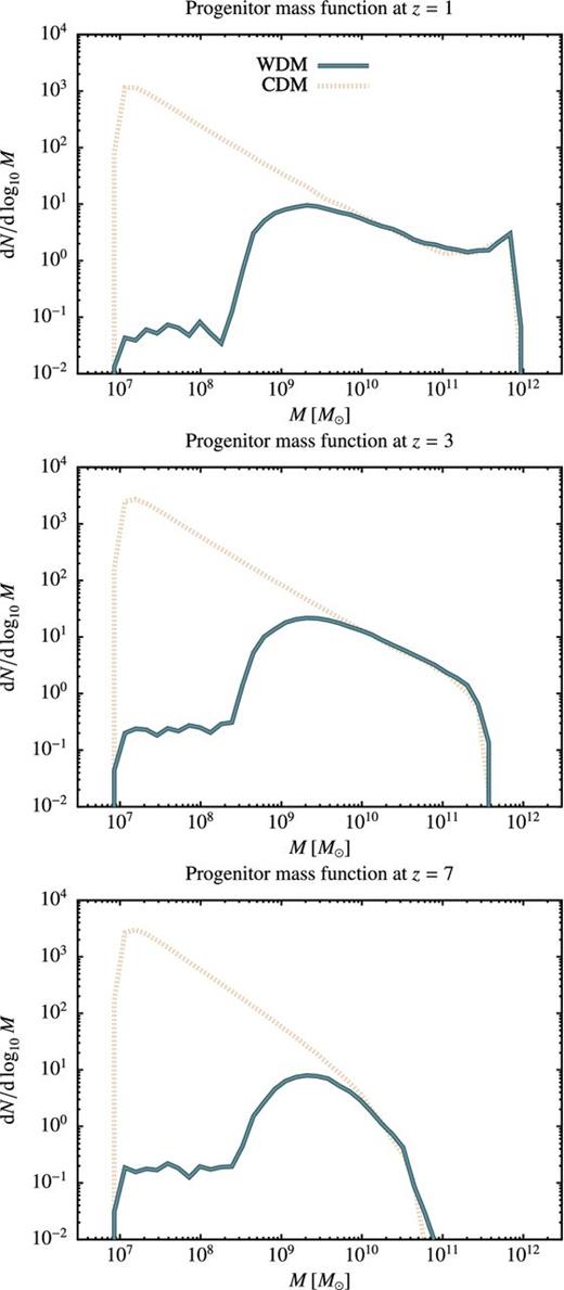
Progenitor mass functions derived via merger tree construction in CDM and WDM cases for a 1012 M⊙ halo at z = 0.
Well below the suppression scale a population of progenitor masses much less than Ms builds up. These are the result of smooth accretion – the first-crossing rate distribution (see Fig. 8) cuts off below Ms, so there is no way for these haloes to arise through branching of the merger tree – which gradually reduces the mass of the lowest mass haloes going back in time. The numerical robustness of our model in this regime is discussed in Appendix B4, in which we also demonstrate that the position of the peak in the progenitor mass function is numerically robust and well determined.
Fig. 11 shows the corresponding mean mass accretion histories of this halo (i.e. the mean mass of the most massive progenitor at each redshift). There is almost no difference between CDM and WDM. This is in agreement with the results of Knebe et al. (2002) who found almost no difference in the mass accretion histories of individual haloes in CDM and WDM N-body simulations. The two haloes presented by Knebe et al. (2002) were significantly more massive (almost 1014 M⊙) than those considered here, but they report the same conclusion for lower mass haloes. They conclude that the number of mergers that contribute significant mass to the assembly of the haloes is unchanged between CDM and WDM case. Our results suggest that this is an accurate conclusion for more massive haloes (the assembly of which will be dominated by haloes well above Ms). However, for lower mass haloes, which gain a significant fraction of their mass from haloes close to Ms, our results clearly show that smooth accretion plays a crucial role in shaping the mass accretion history of WDM haloes – without it, substantial differences from the CDM case would occur.
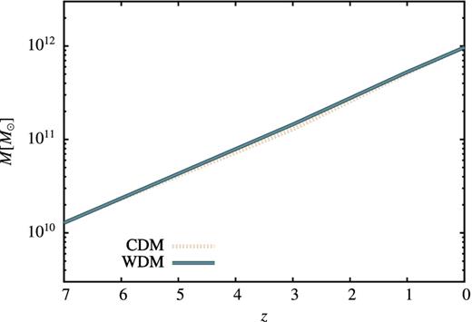
Mean mass accretion histories derived via merger tree construction in CDM and WDM cases for a 1012 M⊙ halo at z = 0.
4 DISCUSSION
We have described algorithms for constructing halo mass functions and merger trees for dark matter haloes in WDM universes. Our methods improve upon previous treatments which did not correctly solve the barrier first-crossing problem (Menci et al. 2012) and which used a top-hat filter to compute σ(M) resulting in an overestimate of the abundance of low-mass haloes. Our results are in excellent agreement with the available N-body simulations. Illustrative results clearly demonstrate that the mass function and progenitor mass functions of WDM haloes are strongly suppressed relative to CDM below about Ms. Differences between CDM and WDM in coarse-grained statistics, such as the mass accretion history, are small for haloes well above the cutoff scale, providing that the accretion of smoothly distributed matter in WDM is accounted for.
The method that we describe has a single free parameter – the coefficient a appearing in equation (6). We have fixed the value of this parameter to match the location of the turnover in the N-body mass function reported by Schneider et al. (2012). This introduces a dependency in one of the simulations to which we compare our model. Nevertheless, as discussed in Section 2.1.1, we expect that the same value of a will be appropriate for all WDM particle masses of interest. The limited evidence available from our present work (i.e. that a chosen to fit the mass function for 0.25 keV WDM also successfully matches the progenitor mass functions for 2.20 keV WDM) certainly supports this claim.
Our approach has the advantage, compared to N-body simulations of WDM, of not being affected by numerical noise in the particle distribution which leads to the formation of large numbers of artificial low-mass haloes (Wang & White 2007) and of being substantially faster to evaluate mass functions and progenitor distributions. Using the techniques developed in this work, the procedure for applying them to dark matter with different phenomenology or to other physics that modifies the power spectrum or excursion set barrier is straightforward:
determine the linear theory power spectrum of density perturbations from the dark matter (or other) physics;
determine, through analytic calculation or idealized N-body simulations, the critical linear theory overdensity for collapse, which will depend on the (thermal and interaction) physics of the dark matter particle.
Given these two inputs our techniques can be used to determine the resulting halo mass function and merger histories of dark matter haloes consistent with the input physics. The accuracy of our methods for phenomenology beyond that exhibited by WDM remains to be tested, but the success in this case leads us to expect that our methods will be generally applicable.
The nature of the dark matter distribution on small mass scales will be investigated by future lensing programmes (Keeton & Moustakas 2009; Vegetti & Koopmans 2009a). The techniques described in this work will allow detailed statistical predictions to be made for the expected numbers and masses of dark matter substructure as a function of dark matter particle properties.
To make accurate predictions for the dark matter subhalo distribution we have addressed only the first part of the problem, namely halo formation and merging. The second part, halo destruction by tidal forces must also be addressed. We plan to explore this process using the methods of Benson et al. (2002a; see also Taylor & Babul 2004), together with prescriptions for the internal structure of WDM haloes (which will, of course, differ from that of CDM haloes; Maccio’ et al. 2012; Macciò et al. 2012).
The methods described in Section 2 have been implemented within the open source semi-analytic galaxy formation code, galacticus (Benson 2012). All results presented in this work were generated using galacticus v0.9.1 r903. Control files and scripts to generate all results presented in this paper using galacticus can be found at http://users.obs.carnegiescience.edu/abenson/ galacticus/parameters/dmMergingBeyondCDM1.tar.bz2.
We thank Rennan Barkana for supplying results from his calculations of halo collapse in WDM universes, and Annika Peter for invaluable discussions and comments on an earlier draft of this paper. The work of LAM was carried out at Jet Propulsion Laboratory, California Institute of Technology, under a contract with NASA. LAM acknowledges support by the NASA ATFP program.
The two usual candidates – both lying beyond the standard model of particle physics – are sterile neutrinos (Dodelson & Widrow 1994; Shaposhnikov & Tkachev 2006) and gravitinos (Ellis, Kim & Nanopoulos 1984; Moroi, Murayama & Yamaguchi 1993; Kawasaki, Sugiyama & Yanagida 1997; Gorbunov, Khmelnitsky & Rubakov 2008).
This scale is usually approximated as being equal to the speed of the particles at the epoch of matter-radiation equality multiplied by the comoving horizon scale at that time; see Bode et al. (2001) for further discussion.
The normalization advocated by Lacey & Cole (1993) is equivalent to a = (9π/2)1/3 ≈ 2.42 which is not too different from our best-fitting value of 2.5.
This fit is accurate for the regime where δc, WDM/δc, CDM < 600, but substantially overpredicts the results of Barkana et al. (2001) for smaller masses. This is a deliberate choice – our aim was to match the shape of the function through the region where it transitions away from the CDM value. On smaller mass scales the suppression is so dramatic that the precise value of δc, WDM/δc, CDM is unimportant.
Note that, as is conventional, we place this time dependence into the critical overdensity, such that we can always work with σ(M) at z = 0. The growth function used here is the usual growth function computed for CDM, consistent with the definitions of Barkana et al. (2001).
This remapping was motivated by considerations of ellipsoidal collapse, the barrier for which differs from that for spherical collapse. In particular, Sheth et al. (2001) noted that the density perturbations leading to low-mass haloes are expected to be more ellipsoidal than those that give rise to the most massive haloes – effectively making the collapse barrier a function of mass scale.
This mapping was derived strictly for the CDM case. We retain it here since for haloes with masses, M, much greater than Ms, we expect the WDM case to converge to the CDM solution. However, there is no guarantee that this mapping remains accurate for M ≲ Ms. In particular, it is possible that low-mass haloes close to the cutoff scale could be more spherical in WDM than in CDM due to the isotropizing effects of the WDM velocity dispersion. Calibration of our methods against reliable N-body simulations of WDM universes would be required to evaluate the accuracy of the remapping in this regime. The N-body simulations currently available and examined later in this work do not address this particular issue as they do not include the effects of the non-zero velocity dispersion of WDM. However, it is understood how to include velocity dispersions in WDM simulations (Brandbyge et al. 2008), and this should be included in future simulations.
That is, the ratio of σ(M) computed using our sharp k-space filter to that computed using the top-hat filter is |$\sqrt{1.197}$|. Note that this scaling factor does not constitute a free parameter in our approach. Instead, it is fixed to offset the change in the S(M) relation on large scales resulting from the difference between top-hat and sharp k-space window functions. Therefore, given a power spectrum and a value of a (the coefficient in equation 6), the scaling factor is directly computable and uniquely determined.
Assuming that σ(M) continues to rise monotonically to arbitrarily small scales. In practice, this is not true as even CDM will have some cutoff in its power spectrum on very small scales (Green, Hofmann & Schwarz 2004; Loeb & Zaldarriaga 2005). However, for our present purposes the assumption that all mass is locked into haloes in CDM is a good one.
The slight difference between this curve and that computed using a top-hat window function is due to our inclusion of the Sheth et al. (2001) remapping. If this were not included, the factor of 1.197 increase in the barrier would precisely compensate for the difference in σ(M) between these two curves on large scales. With the Sheth et al. (2001) remapping included this constant factor cannot correct for the offset fully [due to the non-linear nature of the Sheth et al. (2001) remapping]. Future, high-precision work should consider recalibrating the Sheth et al. (2001) remapping to match a CDM halo mass function with σ(M) computed using our sharp k-space window function. This would obviate the need for a separate multiplicative increase in the barrier and could better capture the scale dependence of the required correction.
Specifically, we adopt a B(S) corresponding to the mass-dependent WDM critical overdensity, but simply use it in the solution for f(S) appropriate to a linear barrier.
The merger tree resolution is limited only by the available computational time and memory. We choose a resolution of 107 M⊙ in this case to be sufficiently below Ms while keeping computing times tractable.
REFERENCES
APPENDIX A: NUMERICAL METHOD
In either case (i.e. equations A13 and A14), solution proceeds recursively: f(S0) = 0 by definition, f(S1) depends only on the known barrier and f(S0), and f(Sj) depends only on the known barrier and f(S<j).
APPENDIX B: NUMERICAL TESTS
In this appendix, we examine the numerical accuracy and robustness of our methods.
B1 First-crossing probability solutions
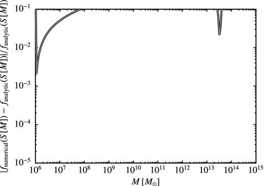
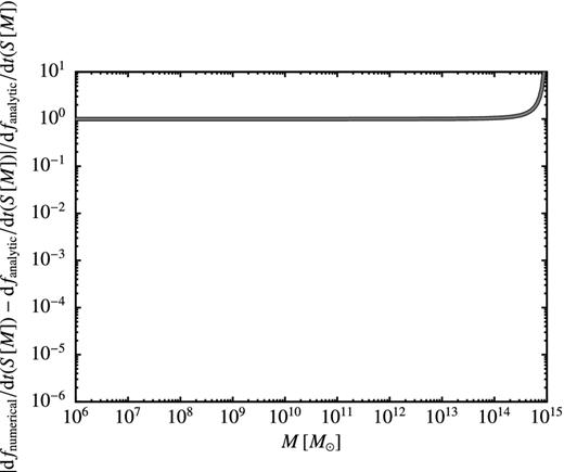
The absolute fractional error in the excursion set first-crossing distribution function, f(S), computed using our numerical method compared to the analytic solution for a constant barrier.
B2 First-crossing rate solutions
The absolute fractional error in the excursion set first-crossing rate function, df(S)/dt, computed using our numerical method compared to the analytic solution for a constant barrier.
B3 Testing the Parkinson–Cole–Helly algorithm on smaller mass scales
The Parkinson et al. (2008) empirical modification to the merger tree branching rate was calibrated against N-body merger trees drawn from the Millennium Simulation. As such, it has been tested for masses above approximately 1010 M⊙. Here we employ the same modification for much lower masses. Fig. B3 compares progenitor mass functions generated by the Parkinson et al. (2008) empirical modification with those extracted from the Aquarius CDM simulations of Springel et al. (2008) which resolve haloes of masses 106 M⊙. It can be seen that the Parkinson et al. (2008) empirical modification performs very well (with unchanged parameter values) for these much lower mass haloes in the CDM case also.
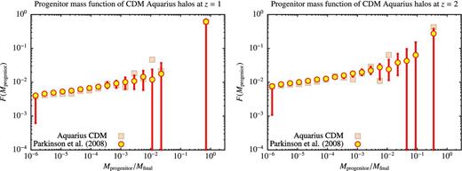
Progenitor mass functions of the Aquarius CDM dark matter haloes (Springel et al. 2008) at z = 1 and 2 (histograms) compared with the predictions of the Parkinson et al. (2008) algorithm. Each panel shows the fraction of the halo mass contributed by progenitors in each mass bin. Masses are shown as a fraction of the final halo mass. The error bars on the predictions from the Parkinson et al. (2008) algorithm indicate the 20th and 80th percentiles of the distribution of progenitor mass functions. While this algorithm was calibrated on the much higher mass haloes found in the Millennium Simulation (Springel et al. 2005), it can be seen to work extremely well at these lower masses also.
B4 Merger tree accuracy and smooth accretion
To test the convergence of our merger trees with respect to the parameter ϵ used in our numerical determination of the first-crossing rate distribution (see Section 2.4), we compute progenitor mass functions of 1012 M⊙ haloes for ϵ = 0.010, 0.003 and 0.001. Additionally, we perform these calculations both with and without the smooth accretion term of Section 2.5.1.
Fig. B4 shows progenitor mass functions at z = 1, 3 and 7. When smooth accretion is included, the WDM progenitor mass function closely matches that of CDM above about 3Ms, but is strongly suppressed below it at lower masses. If smooth accretion is ignored the WDM progenitor mass function evolves much more slowly and diverges from the CDM case even at the highest masses. Ignoring this smooth accretion leads to significantly biased results.
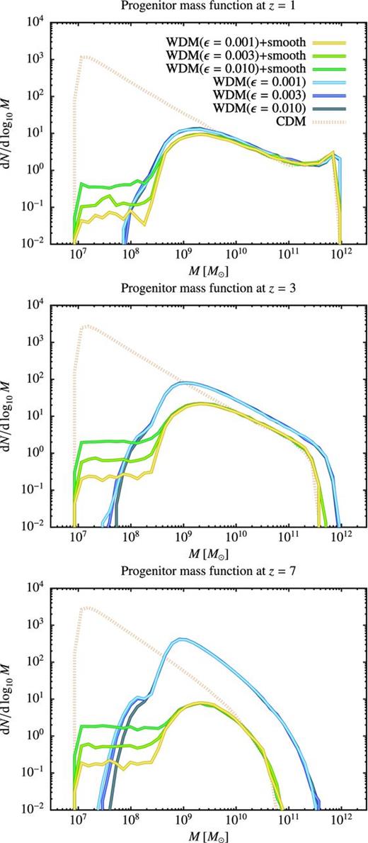
Progenitor mass functions derived via merger tree construction in CDM and WDM cases for a 1012 M⊙ halo at z = 0. For the WDM case, results are shown for different values of ϵ and also for cases with and without the accretion of smoothly distributed matter.
It can clearly be seen that our WDM results are converged with respect to the ϵ parameter except at masses well below the suppression scale in the progenitor mass function in the cases where smooth accretion is included. Here, a population of progenitor masses much less than Ms builds up. These are the result of smooth accretion – the first-crossing rate distribution (see Fig. 8) cuts off below Ms, so there is no way for these haloes to arise through branching of the merger tree – which gradually reduces the mass of the lowest mass haloes going back in time.
Our numerical determination of the first-crossing rate function is currently not robust in its determination of smooth accretion rates for these lowest mass (highest variance) haloes where the excursion set barrier is a very rapidly changing function of variance and our discretization of S used to obtain a numerical solution inevitably does a poor job of resolving the barrier. This could of course be mitigated by using a yet smaller value of ϵ (requiring substantially increased precision in the numerical solutions) or a finer grid in S (requiring both increased precision and substantially more computing time). Nevertheless, the position of the peak in the progenitor mass function is well determined, and the differences in the abundance of low-mass progenitors have negligible effect on the mean mass accretion histories of haloes considered in this work.
