


Abstract
In this article a 2-level multinomial model for the calculation of Likelihood Ratios (LRs) as a measure of the strength of evidence in the case of categorical evidence is introduced. In order to illustrate its usage, it is applied to gunshot residue (GSR) comparison data obtained in an experimental set-up and analysed using electron microscopy. The data consists of a number of gunshot residues divided in k categories depending on their elemental composition. For comparison a score-based model (the Pearson correlation) and a 1-level multinomial model estimated with Maximum Likelihood (ML) were also applied on the same data. Three variations of the 2-level multinomial model were tested, together with the other two models. The results show that all tested models can be applied on categorical data such as GSR. The 2-level multinomial model, the model that is introduced in the study, shows the least misleading evidence. Furthermore this article demonstrates a first step taken towards a system that calculates numerical LRs in GSR comparison studies.
1. Introduction
The comparison of two or more items of evidence is the core business of forensic scientists. Examples are: Comparing DNA of a suspect with that on the crime scene, or comparing glass in the hair of a suspect with that on the crime scene. The general question of interest for the court is whether these pieces of evidence originate from the same source. Nowadays it is widely accepted that forensic experts generally cannot fully answer such a question, because other information is needed which mainly lies outside the field of expertise of the particular expert. However, experts can provide a measure for the strength of the evidence under their investigation. This measure of strength of evidence can be quantified by a Likelihood Ratio (Robertson and Vignaux, 1995; Evett, 1983, 1998; Champod, 2000; Aitken and Taroni, 2004). The Likelihood Ratio (LR) applied to forensic sciences, is the ratio of the probability of finding certain feature values under two competing hypotheses, often referred to as the prosecutors and defence hypotheses. The prosecutor’s hypothesis (in the numerator) generally states that two items come from a same source while the defence hypothesis (in the denominator) states that two items come from different sources. The LR is usually expressed verbally, as in ‘observing this profile is more probable if it comes from the suspect than if it comes from a random person’. More and more research is performed to produce also numerical LRs, as in ‘observing this profile is a 100 times more likely if it comes from the suspect than if it comes from a random person’. Numerical LRs could be used as such in the report or form the scientific base of the reported verbal scales.
To calculate numerical LRs, data and statistical models are needed. In LR modelling two main strategies can be chosen, one based on score-based models and one based on feature-based models. For these models the same raw data in the form of feature values can be used, but the resulting LRs are fundamentally different (Bolck et al., 2015). Score-based models calculate LRs based on univariate scores in the form of distances or similarities between the feature values. They generally investigate whether items come from same sources or not. Feature-based models calculate LRs on the complete multivariate structure of the feature values to investigate whether a requested item comes from a specific source or not. The focus in this article is on these feature-based models. Different feature-based models exist based on the type of data used, as shown below.
There are the models for discrete data (Aitken and Gold, 2013). Discrete data is data with features that can take one of a limited number of values (such as DNA, counts, or colours and shapes of objects). DNA profiles consist of the numbers of base-pair repetitions at various loci. These profiles are a special form of discrete data because DNA in various cells of a single person generally is identical, so there is no within-source variation. Therefore the numerator of the LR of comparing single DNA profiles equals one. The denominator equals the ‘match probability’ (Selvin et al., 1983), which can be estimated by the frequency of occurrence in a relatively small sample. Also for DNA, by assuming approximate independence between the frequencies of the separate loci, the frequency of the whole profile is obtained by multiplying the frequencies of the individual loci, apart from a small correction factor. LRs of such multivariate profiles with independent features, whether they are based on discrete data or other types of data, can be obtained by multiplying the LRs of the individual (univariate) features.
Continuous data, such as a refractive index or chemical profiles, do have within source variation due to noise in, e.g. the elemental composition of glass fragments of the same window. As a result the numerator of the LR that does not equal one. Also probability density functions, instead of probabilities, should be used in the denominator as well as the numerator. Continuous data such as chemical profiles are multivariate and unlike the DNA profiles have dependent features within the profile. In that case multivariate densities should be used. For these type of data 2-level models were introduced (Aitken and Lucy, 2004; Zadora et al., 2014).
Yet another type of models, are models based on categorical data with more than 2 categories. In contrast to DNA-type discrete evidence that take one of a fixed number of possible values, categorical evidence consists of counts or proportions in categories. Aitken and Gold (2013) describe models for counts of characteristic occurrences in certain time periods. Counts, or proportional data derived from it, in multiple categories can be seen as multivariate discrete data. An example of such kind of data is gunshot residue (GSR) data. These data consists of inorganic GSR particles that are formed after discharging a cartridge with a firearm. The elemental compositions can be considered as counts of particles assigned to k particle categories, such as PbBaSbSn, GdZnTi, BaSb and ZnTi (Stamouli et al., 2008; ASTM E1588). Thus GSR data consists of count data that can be considered as counts in k categories that vary between samples of a same source and differ between samples of different sources. This article introduces feature-based LR models for categorical data based on the multinomial distribution. As an example these models are applied to a limited set of GSR data, but can also be applied on other type of categorical data.
The presented feature-based models based on multinomial distributions are compared with a score-based model that relates to the research recently performed in the field of forensic GSR comparisons (Rijnders et al., 2010). In the past years various groups in this field have done research on discriminating ammunition types based on GSR compositions. One of the important aspects with performing comparison studies is to estimate the frequency of occurrence. Data such as shown by Charles et al. (Charles et al., 2011) can be used. Recently the authors have published on the building of a database containing elemental compositions of cartridge cases originated from criminal cases. Others have tried to associate GSR samples from a crime scene with the type of ammunition used by analysis of the GSR compositions, notably the work of Brozek-Mucha and Jankowisc (2001), Brozek-Mucha and Zadora (2003) and Steffen (2006). The current article is, with respect to the GSR data, a continuation of the work of Rijnders et al. (2010). Here, it was shown that the Pearson correlation could discriminate between same-ammunition-type GSR compositions and different-ammunition type compositions. Therefore, the feature-based LR models presented in the current article are also compared with a score-based model based on the Pearson correlation distance. Focus will be on the feature-based models. The GSR data are too limited for practice, but are only used to illustrate that the models may work also when compared to the above-mentioned score-based model. In Section 2 the data are introduced, followed by the description of the models in Section 3. In Section 4 the results and discussion can be found and in Section 5 the conclusion is formulated.
2. Data and experimental setup
Experimental data are used to illustrate the theory in this article. These data are limited and do not cover all aspects needed for practical use, but are suitable for demonstrating the developed models. The data are an extension of those used in (Rijnders et al., 2010) and are gathered over a period of four years. In total 53 shots were fired using 13 different ammunition types. The number of shots per ammunition type is presented in Table 1. Three of the ammunition types (Magtech, S&B and Action Effect) were shot in 2 series with years in between those series.
Summary of the number of shots per ammunition type (including abbreviations which we used in Figs 3 and 4)
| Ammunition type (abbreviation) | Number of shots | |
|---|---|---|
| 1 | Samson Ultra (Sam) | 2 |
| 2 | Magtech (Mag) | 6 |
| 3 | Winchester (Win) | 2 |
| 4 | Lawman (Law) | 2 |
| 5 | S&B (S&B) | 10 |
| 6 | Action Effect (AE) | 7 |
| 7 | Sintox (Sin) | 4 |
| 8 | HP 6.35 (HP) | 4 |
| 9 | Remmington (Rem) | 4 |
| 10 | CCI (CCI) | 4 |
| 11 | Spreewerk (Spree) | 4 |
| 12 | Geco (Geco) | 2 |
| 13 | Fiocchi (Fio) | 2 |
| Total | 53 |
For each shot GSR were collected from various locations, of which 2 are used in this article. The collection of GSR from a location simulating the hand of the shooter was performed by placing a stub1 near the gun (the term ‘hand’ for short is used in the remainder of this article). Another stub was used to sample an entrance bullet hole which was shot at 60 cm in front of the gun simulating the clothes of the victim (the term ‘victim’ for short is used in the remainder of this article).
GSR particles collected with half inch aluminium stubs having an adhesive carbon tape were analysed by Scanning Electron Microscopy/Energy Dispersive X-Ray Spectrometry. The analysis was performed with FEI electron microscopes using an Oxford EDS detector equipped with INCA software of with an EDAX detector equipped with the GSR Magnum software.
GSR are particles that are formed when discharging a cartridge with a firearm and consists of single or a combination of chemical elements. In forensic comparison their elemental composition is used to make comparison studies, because the variation in elemental composition between ammunition is quite large. The variation in elemental composition of ammunition is the result of using different materials for the various parts of a cartridge. For example when the cartridge Action Effect is used, GSR particles containing the elements Gd, Zn and Ti as well as GSR particles containing Zn and Ti and single components (Gd, Zn and/or Ti) are created and expelled from the firearm. One of the largest contributions of GSR is the primer. Different primers are available, ranging from non-toxic (without the presence of heavy metals e.g. ZnTi) to marked primers (used from police officers e.g. ZnTiGd). The GSR composition can be seen as a list of (k) categories, representing counts of particles in k particle type categories (see Fig. 1).
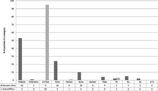
Examples of the GSR composition of observations of two different ammunition types (Samson Ultra in dark grey and Action Effect in light grey) with k = 12 particle type categories. Percentages of various particle types (on the x-axis) for the two ammunition types are provided on the y-axis. Some compositions do add up to 99 or 101% (instead of 100%) due to rounding.
In this article the number of categories are fixed to k = 12. In GSR practice the number of categories may vary from case to case. That is no problem as long as the items to be compared and the background in one case have the same categories. To illustrate the theory, the 12 categories selected in this article are: PbBaSb, PbBaSbSn, GdZnTi, PbSb, Sn, BaSb, BaSbSn, PbBa, Pb, Ba, Sb and ZnTi. If particles included some other elements attached to one of these 12, such as Al or Zn, they were assigned to the corresponding basic category without that extra element (e.g. PbBaSbAl and PbBaSbZn are both assigned to PbBaSb).
To calculate a LR as a measure of strength of evidence, in general three types of data will be distinguished. Firstly, a control or reference data (X) consisting of one or more measurements within one source. In this article these concern GSR compositions of several shots with the same ammunition type. Secondly, questioned or recovered data (Y) consisting of one or more measurements of unknown source to be compared with the control. Here, these are individual GSR compositions. Thirdly, the background data (Z) consisting of measurements of many sources representing the population. Here all 106 GSR compositions of the 53 shots sampled at the two different locations (‘hand’ and ‘victim’). Within this background data, the combination of ammunition type and location were used as a source. This means that in this article we have 2 locations times 13 ammunition types. That is 26 separate ‘sources’. Summarizing, to illustrate and test the presented models, the above-described GSR data were used as follows:
Control X: All GSR compositions of one specific ammunition type and one location can be used as a control. Thus in total there are 2 × 13 = 26 separate controls. For each control there are at least two measurements (shots) of which the mean is used as the reference composition.
Recovered data Y: All individual GSR compositions of all 53 shots at the two locations ‘hand’ and ‘victim’. Thus in total there are 106 GSR compositions for comparison with a control (resulting in106 separate LRs).
Background data Z: GSRs compositions of all the 53 shots, with 13 ammunition types, measured at the two locations ‘hand’ and ‘victim’. Thus in total there are 106 GSR compositions divided over 13 ammunition types and two locations, representing 26 sources.
Note: for the control and recovered data the same data are used as for the background. Preliminary calculations were performed by dividing all data in separate test- and training sets and also by removing the control and recovered under calculation from the background. These calculations resulted in LRs of the same magnitude as those shown in this article. Therefore and because in practice you may not know whether your control or recovered are present in the database, it was decided to use all data in the above way to gain a large number of (LR) results.
All statistical calculations were done in R (http://www.r-project.org/).
2.1 Data pre-treatment
In GSR studies the focus can be on the total number of GSR particles (Cardinetti et al., 2006, Gauriot et al., 2013, Biedermann et al. 2009 and 2011), which may have evidence in itself. The focus of the current article is, however, on the relative contributions of particles, that is the GSR compositions, whatever the total number is. Therefore, the number of particles in categories per sample in this article is normalized to a fixed total of 100%, resulting in a composition of relative proportions or particles per category. Based on this the strength of evidence was determined.
3. Models
This LR sometimes simply can be calculated by the frequency of occurrence of E (e.g. the logo on XTC tablets or DNA at one locus) under the two hypotheses. However, often the evidence consists of multiple and/or continuous features or other complicating aspects such that more complex statistical LR models are needed. This article focuses on models for such type of data; categorical or count data in more than two categories. These models are presented in the sections below.
The theory about the LR models for categorical data below were applied to GSR data to illustrate them. Currently, GSR experts in the Netherlands compare two (or more) GSR compositions visually and evaluate their (dis)similarities with verbal LRs,2 based on expert knowledge and experience, with respect to the hypotheses related to the same shot (Hp) or another shot (Hd).
There are several aspects to (GSR profiles) that influence the discrimination between the above hypotheses. One aspect is the variations within and between ammunition types; another aspect is the variations due to the location of sampling. Finally one has also to consider the memory effect. Memory effect is the phenomenon where GSR from a previous shot is expelled from the firearm at a following shot. The experimental data used in this article do not cover all these aspects. They are an extension of the data used in (Rijnders et al., 2010), where measurements were performed with a selection of ammunition types at sampled from various locations. The focus in the experiment in that article was investigating whether it is possible to statistically discriminate between ammunition types based on GSR compositions. Therefore, the memory-effect of the weapon was reduced as much as possible by cleaning the weapon thoroughly after each shot. In (Rijnders et al., 2010) it was shown that, among other things, Pearson correlation coefficients based on GSR compositions can be used to discriminate between ammunition types. In the current article we want to test whether the used models can be used to calculate the strength of evidence for discriminating between ammunition types, rather than discriminate between shots. Therefore, instead of the above hypotheses of GSR practice, we used variations of the more general hypotheses3:
Hp: GSR Y has the same specific ammunition type as X
Hd: GSR Y has a different ammunition type than X
3.1 Score-based LR models
The numerator gives the density of the score between two items using the distribution of comparison scores within sources and the denominator gives the density of the same score using the score distribution between sources. The score, instead of the original features, is used as the ‘evidence’ of which the strength of evidence is calculated with a LR. This score evidence generally is used to differentiate between common and different sources, instead of between a specific same source and another source. If within source variation may be assumed more or less equal (homogeneous intra-batch distributions (Meuwly, 2001)) this can be done and has the advantage that per comparison the same background can be used and this more data is available. This data consists of same-source comparison scores of various sources aggregated and different-source comparisons over various sources. If desired it is also possible to differentiate between a specific source and another source, but without the above mentioned advantage.
In forensic expertise’s with evidence consisting of many features, such as in speaker recognition (Brümmer and De Preez, 2006), or in fields where features cannot be easily measured themselves, e.g. finger traces (Neumann et al., 2007; Egli et al., 2007) or handwriting (Hepler et al., 2012), LRs based on scores then can be very useful or even the only option. The disadvantage of score-based models is that they generally reduce the whole multivariate structure of the evidence to one univariate measure. This means possibly information-loss including the information on dependencies between the various features and the information on the rarity of the profile. Apart from this information loss, not including rarity and using different hypotheses, score-based models (in contrast to feature-based models) are in general more robust, and do not have estimation problems due to high dimensionality. This is elaborated in (Bolck et al., 2009, 2015).
In a previous article (Rijnders et al., 2010) it was shown that using the Pearson correlation discrimination between ammunition types was possible. So it can be expected that a score-based LR based on the Pearson correlation or Pearson correlation distance (as in (Bolck, et al., 2009)) can distinguish between ammunition types. Therefore, in this article, a score-based LR model based on the Pearson correlation distance is used as a reference to which the developed feature-based models are compared. In the above formula, (x, y) thus is , with r the Pearson correlation between the samples x and y, with x = {x1,x2,…,xk} and y= {y1,y2,…,yk} vectors with count data (xi and yi) in k categories.
All scores of same-source comparisons and different-source comparisons are smoothed using Kernel Density Estimation (KDE), with a Gaussian kernel and optimal bandwidth (Silverman, 1986).
3.2 Feature-based LR models
With the numerator of the last term the conditional density of a recovered profile given the distribution of profiles within the specific source that is compared with and in the denominator the density of the recovered profile given the distribution of profiles in the population of sources. In contrast to score-based models, the whole multivariate structure of the data is considered and with that the rarity of a profile with a certain multivariate structure. In this way, more information is considered. On the other hand, a complex structure often needs complicated calculations and therefore problems with calculating measures of association in high dimensionality may occur.
Below a description is given of possible feature-based LR models for multivariate categorical or count data is given.
3.2.1 Feature-based models based on multinomial distributions (1-level)
With , πXi representing e the probability of (a particle) falling in category i if it comes from source X, and πi representing the probability of falling in category i if it comes from the general population of sources. Conditional Independence of the individual observations of particles is assumed.
The LR gives the probability of finding a measurement y if this measurement comes from the same source as X compared to the probability of finding this measurement y in the general population. In general the values πiand πXiare not known. They can be estimated, for instance with Maximum Likelihood (ML), by sample values piand pXi from representative samples. Alternatively, prior distributions on the probabilities can be assumed. This Bayesian or 2-level approach is presented in the next section.
3.2.2 Feature-based LR models based on multinomial distributions with priors (2-level)
With, f(θ) the prior distribution of the parameters θ representing the variation in θ across the population of all possible sources. Within one source these priors can be updated with the control data x to a posterior distribution f(θ|x). This results in a LR with a numerator representing the posterior predictive distribution of a new measurement y, and a denominator of a prior predictive distribution of this new measurement (Bolck et al., 2009; Bolck and Alberink, 2011).
With , , , and the gamma function.
The Dirichlet distribution is the multivariate alternative for a beta distribution. The beta distribution is commonly used as a conjugate prior in case of only two categories (k = 2), when the multinomial distribution equals the binomial distribution (such as with DNA).
With and .}
The (hyper) parameterscan be thought of as prior observation counts. There are various options for hyperpriors on these parameters:
; This is a uniform prior for π. This is not very practical in this case, because the background data measurements are then ignored. On the other hand this may not effect results to a high extend.
. This is a Haldane prior or uniform prior for log(π). This is an improper prior and also not very practical in this case, for the same reason as 1.
; This is a Jeffrey prior, a special kind of non-informative prior. In contrast to the uniform prior this prior is invariant under one-to-one transformation of the parameters, but again it is not very practical in this case, for the same reason as 1.
Use a mixture of Gamma or comparable distributions or other distributions on . The problem is that its parameters will need priors too, and so on.
Use of MCMC (Markov Chain Monte Carlo; A method often used in Bayesian analyses for sampling from probability distributions) or comparable iterative processes (e.g. (Gelman et al., 2004; Congdon, 2005)).
Approximating with and ; If is taken and pi is estimated from the mean proportions in the background data, thenrepresent the counts normalized to percentages.
- In case of k = 2 (binomial distribution with beta prior) the parameters 1 and 2, can be estimated with Maximum Likelihood (ML) based on background data representing the population of all sources:
With , and N the number of sources, pj the probability to be in the first of the two categories of type j and (1–pj) the probability to be in the second category. If more than two categories are considered no closed-form ML estimators for the hyperparameters exist. In that case, ML estimators can be approximated with iterative processes (such as Newton-Raphson or Expectation Maximization (EM)) to find optimized estimators (Minka, 2003; Ronning, 1989). In this article, optimal hyperpriors based on the optimization of the log-likelihood of the Dirichlet function with the Quasi Newton iteration method L-BFGS-B within the software package R are used (Ronning, 1989). The log-likelihood function is: with
Other options of course are possible. A selection of the above, as described in subsection 3.3, is used to calculate LRs to illustrate the effect of the various model choices. MCMC is not selected in order to keep the models simple for this initial investigation.
3.3 Selected models for demonstration
Five LR models for categorical data were selected and applied to the gunshot residue data of Section 2 (with their abbreviation between brackets):
A score-based model based on a Pearson-correlation distance smoothed with KDE, because previous research was based on this (Rijnders et al., 2010) (Pearson).
A 1-level feature-based model with a multinomial distribution for the control and another multinomial distribution for the background based on ML estimation, because this is perhaps the most intuitive model and a direct extension of simple discrete models based on binomial distributions (ML).
A 2-level model with a multinomial within distribution and a uniform prior (Uni).
A 2-level model with a multinomial within distribution and a mean prior using and =100 and pi is estimated from the mean proportions in the background data Z. (Mean %).
A 2-level model with a multinomial within distribution and an optimal prior for } based on the background data Z according to (Ronning, 1989) as described in point 7 above (Optim).
In Section 4, LR calculations using the same GSR data with all five selected models are presented. The results are visualized with boxplots in order to visualize the variations in LR values. Important is the general information these boxplots give with respect to median values (variation within the LR values) and for comparison reasons, rather than the exact values of the LRs. These latter may change when the background data is larger and more representative and when the models are calibrated and adjusted to specific casework. Tables of misleading evidence are provided, presenting percentages of LRs smaller than 1 for (known) same-source comparisons and LRs larger than 1 for (known) different source comparison. Thus providing global percentages of LRs pointing in the opposite direction as expected. The models are too general for performance measures such as ECE plots uses.
4. Results and discussion
In this section, five selected LR models for multivariate categorical data are applied to GSR comparisons as an illustration. These five models are referred to using the abbreviations as presented between brackets in subsection 3.3. The GSR compositions used are part of the experimental data as described in Section 2 and consist of proportions in 12 categories. Within this data the ammunition type (in total 13 types) and the location sampled (the hand of the shooter or at the body of the victim) of all profiles was known. Based on this the LR results can be divided into three situations: (1) LRs related to GSR compositions of same ammunitions at a similar location (e.g. thus both GSRs come from the hand (1a) or both from the victim (1b)); (2) LRs related to GSR compositions of same ammunitions but different locations and (3) LRs related to GSR compositions of different ammunition types. It is investigated whether the LRs can discriminate between ammunition types (at the same and different location) and how well this was done.
In subsection 4.1 results in the form of LRs and misleading evidence of all possible comparisons are combined and presented for the five models and the above situations. In subsection 4.2 comparable results per ammunition type are presented for two of the five models to illustrate the variation in LRs per ammunition type. In subsection 4.3 the robustness of the models is investigated. In subsection 4.4 the results are discussed.
4.1 LRs and misleading evidence for all 13 ammunition types together
For all five models the same data were used (see Section 2). The recovered data (Y) consist of 106 GSR compositions (of k = 12 categories) that each are compared separately with all 26 controls (X). The control compositions (with the same k = 12 categories) are the means of 2–10 shots within the same ammunition type at one location. In total thus 106 × 26 = 2756 comparisons are performed, of which 53 are same-ammunition type at the location ‘hand’, 53 are same-ammunition type at the location ‘victim’, another 106 are same-ammunition different-location type, and the remaining 2544 are different-ammunition type comparisons. The different-ammunition type comparisons are at the same location as well as at a different location. The background data (Z) consist of the same 106 GSR compositions as the recovered data, but grouped in m = 26 sources (13 ammunition types at 2 locations), as described in Section 2.
Means of multiple (often 2) control measurements are used instead of individual measurements, because this is expected to make LR calculation more robust. This is not conform GSR practice, because in practice usually there is only one measurement of unknown origin. The data used are intended to illustrate that the proposed models, rather than to provide the perfect model for GSR investigation. Even so, in subsection 4.3 the difference between using means or individual measurements is investigated in more detail.
The LRs calculated with the feature-based models are based on the hypotheses as presented in Section 3, assuming GSR Y to come from the same specific ammunition-type as GSR X or another ammunition-type, and thus calculating new model values for each control. The score-based models assume X and Y to come from same or different ammunition-types in general. These slightly different hypotheses are chosen because these are generally used for score-based models. They have the advantage that model values need to be calculated just ones for all comparisons and all the available data can be used for that. This gives more robust LRs than when exactly the same hypotheses are used. In this way all differences between score-based and feature-based models can be investigated. The hypotheses for all the earlier mentioned three situations are (per model type) the same. We designed the experiments, thus we know what samples come from the same ammunition and/or location and what samples do not. In real cases this is of course not possible.
The distributions of the LLRs, that is the logarithm with base 10 of the LRs (thus log10LR or 10log(LR) as is used in the figures), of all 2756 comparisons for each of the five models are illustrated with box-plots4 in Fig. 2 per situation.
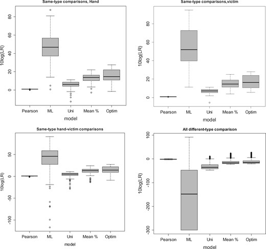
Boxplots of LLRs calculated with 5 models based on 13 ammunition types at 2 locations; Above the same-ammunition type comparisons with both X and Y measured on the hand of the shooter (left) or both X and Y measured on the victim (right). Below same-ammunition type comparisons at different locations (‘hand’ or ‘victim’) (left) and different-ammunition type comparisons (right).
Table 2 gives the corresponding misleading evidence (frequencies with total numbers between brackets) for the five models at the four situations. Here false negatives (FN) are LRs below 1 and thus LLRs below 0 in same source comparisons. Thus, where positive LLRs are expected. False positives (FP) are LRs larger than 1 or LLRs larger than 0 where negative LLRs are expected.
Frequency of misleading evidence corresponding to Fig 2; with between brackets the numbers of the in total 2 times 53, 106 and 2544 comparisons, or each of the four columns
Frequency of misleading evidence corresponding to Fig 2; with between brackets the numbers of the in total 2 times 53, 106 and 2544 comparisons, or each of the four columns
Not presented, but also investigated, was the effect of the various models on LRs of individual comparisons in contrast to the aggregated results of the boxplots above. It was found that the score-based model almost always provided the lowest LR (in absolute terms), and that the feature-based models often followed the same pattern in LR values in the sense if one model provided a low LR another model did the same. The highest values (in absolute terms) where almost always provided by the ML model, but this model also showed the most variation.
4.2 LRs and misleading evidence for all 13 ammunition separate
In this section the same LLRs as in subsection 4.1 are presented in boxplots, but now per ammunition type (Figs 3 and 4). This is done for only two models instead of five, to limit the number of figures. More pictures will not add to the purpose of making clear that LRs may vary between the ammunition types. Care has to be taken with the interpretation of the boxplots though, because for some ammunition types only two measurements were available (see Table 1). This means that some boxplots for same-ammunition type comparisons are based on only these two measurements. No misleading evidence is presented for the same reason.
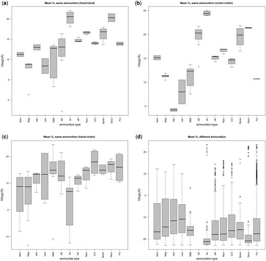
Boxplots of LLRs calculated per ammunition type with the MEAN model at two locations; In the upper pictures same-ammunition type comparisons with both GSR compositions measured on the hand of the shooter (left) or both on the victim (right) are shown. The lower pictures show same-ammunition type comparisons at different locations (‘hand’ or ‘victim’) (left) and different-ammunition type comparisons (right). The abbreviations of the various ammunitions can be found in Table 1.
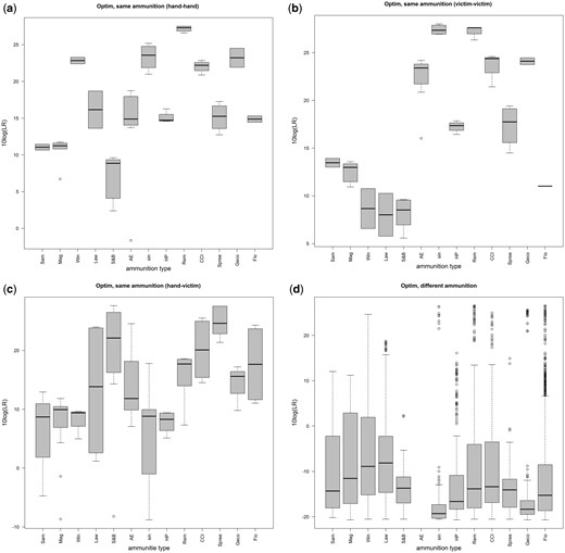
Boxplots of LLRs calculated per ammunition type with the OPTIM model at two locations; In the upper pictures same-ammunition type comparisons with both GSR compositions measured on the hand of the shooter (left) or both on the victim (right) are shown. The lower pictures show same-ammunition type comparisons at different locations (‘hand’ or ‘victim’) (left) and different-ammunition type comparisons (right). The abbreviations of the various ammunitions can be found in Table 1.
4.3 Robustness
The boxplots in subsection 4.1 show that LRs within one ammunition type (and location) can differ a factor 10 or 100. LRs calculated with the ML model even show larger differences (e.g. form LLR 5–10). This model seems with that respect the least robust.
Robustness as a result of reducing the background data was also investigated. The results showed that a reduction of the background data by 10–20% did not affect the magnitude of the LR values.
The effect of the number of measurements per control was investigated as well. Above LRs are calculated based on the mean of all measurements per control to demonstrate the models in general. In most cases in GSR practice only one control measurement is used. Figure 5 illustrates the effect of reducing the number of control measurements on LR values. On the y-axis the LLR is given of ten S&B ammunition measurements (numbered on the x-axis) when comparing with a control based on the mean of 10 measurements (black line), five measurements (dashed line), two measurements (dotted line) and all single S&B measurements separately (this is shown with dots, and no line). These figures are provided for the models Mean (left) and Optim (right) and recovered at location ‘hand’. They show that using the mean of 5 rather than 10 measurements does not seem to effect the LRs much. Using only one measurement shows high variation in the LR values. This is something GSR experts need to be aware of. The same pattern can be seen with other models and other ammunition.
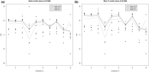
Same-ammunition and location LLR values calculated with models MEAN (left) and OPTIM (right) of which all 10 (recovered) S&B GSR profiles (on the hand) are compared with S&B controls based on the means of 10 (straight line), 5 (— line) or 2 (dotted … line) measurements, or 10 individual values (various symbols, without lines)(also on the hand).
4.4 Discussion
Figures 2–5 show that the score-based model provides relatively low LRs compared to feature-based models. The LRs based on the Pearson correlation are almost all between –10 and 10, which correspond to (only) the first two levels of the verbal scales in the footnote of the model Section 3. All feature-based models show more variation and thus also much higher values in absolute terms. This is seen before in similar situations (Bolck et al., 2009, 2015) and probably due to the fact that score-based models reduce the multivariate structure of the profiles of 12 categories to a single distance measure resulting thus in information loss. Another consequence of this is that in most cases, also in this article, score-based LRs are more robust against small variations within the data. This effect can partly be seen in the boxplots of Fig. 2. The score-based model (Pearson) has a thinner box than all feature-based models and especially the 1-level model with the parameters estimated by ML. This latter model produces high LRs that vary a lot with every small change. The robustness of all models reduces when (means of) less control measurements are used.
Misleading evidence as shown in Table 2 is very low for all models comparing same sources at the same location. False negatives when comparing same ammunition types at different locations are slightly higher especially for the Uni and ML model. False positives vary from 8% to 18%, with the highest percentage for the Pearson model and the lowest for Uni. The 2-level feature-based models Mean and Optim have moderate misleading evidence on both sides and are perhaps overall the best. Part of the misleading evidence can be explained by the not yet representative background data and the memory effect. This effect is related to the release of GSR particles with a composition that is not compatible with the composition of the primer of the ammunition, but with primers of ammunition which have been previously fired from the firearm (Charles et al., 2011; Zeichner et al., 1991).
5. Conclusion
This article presents models developed to calculate numerical LRs for multivariate categorical data. Three variants of a 2-level multinomial model (abbreviated: Uni, Mean and Optim) are introduced and comparable to those for multivariate continuous data (Aitken and Lucy, 2004, Aitken et al., 2007). This 2-level multinomial model was compared with a simple 1-level multinomial model (abbreviation: ML model) and a score-based model based on the Pearson correlation distance (abbreviation: Pearson) between two profiles.
The 5 models are used with experimental GSR data that are an extension of the data used in the former GSR paper (Rijnders et al., 2010). The data consists of GSR particle counts normalized to proportions in 12 elemental composition categories. LR results suggest that all presented models are reasonable options for calculating LRs for categorical evidence. In detail the results are summarized in Table 3. This table shows that models differ to a lesser or greater extend in various aspects.
Characteristics of 5 selected LR models (see subsection 3.3.) for categorical data; First some general statistical properties are summarized followed by three columns of summarizing results based on the calculations on the GSR dataset presented in this article. The labels + (very robust), – (not robust at all) and +/– (in between) are classifications relative to each other and based on the boxplots and discussion in subsection 4.1–4.3. Concerning misleading evidence: There were hardly any same-location false negatives (at the most one). Therefore only FP and different-location FN were provided
| Model type | Model abbreviation | General/statistical | Range LLR values | Robust | Misleading evidence |
|---|---|---|---|---|---|
| Score based | Pearson | Loss of information due to scores; rarity not included. | (–4,1) | + | 17% FP |
| Common/specific same-source | (5% diff-location FN) | ||||
| 1-level multinomial | ML | 1-level feature based; curse of high dimensions | (–300,95) | – | 13% FP |
| (11% diff-location FN) | |||||
| 2-level multinomial | Uni | curse of high dimensions; Non-informative priors | (–48,11) | +/– | 8% FP |
| (18% diff-location FN) | |||||
| Mean % | curse of high dimensions; | (–23,25) | +/– | 13% FP | |
| Informative priors | (7% diff-location FN) | ||||
| Optim | curse of high dimensions; Informative priors | (–21,28) | +/– | 16% FP | |
| (7% diff-location FN) |
The data and models are not fully extended and adapted for practical GSR comparison. As far as the authors are aware no models for LR calculation on full GSR data for comparison reasons are developed yet, so this arfticle presents a starting point. Future research concerning evidence evaluation in GSR comparisons will concentrate on creating a larger more representative background dataset, which may lead to more accurate LR values. Models need also to be refined and improved, perhaps calibrated, using the feature-based 2-level model with mean or optimized hyperpriors. Robustness issues concerning lack of the number of repeated measurements have to be addressed. Hypotheses on the identification level (GSRs originate from same shot versus GSR originate from different shots) need be considered. Data on shot level, incorporating memory effect, will be developed and compared with expert opinions in order to make the step towards calculating numerical LRs for actual casework in gunshot residue comparisons.
The main objective of this study was the introduction of the 2-level multinomial model for categorical data. As shown in Table 3 this model type can be applied on such data. Various options for (the parameters of) these models can be used. Which ones are more suitable in specific cases should be investigated more deeply in those specific cases. In this article, the differences for instance in misleading are not large and also should be further investigated with more and representative data for the specific cases at hand.
Footnotes
1A sampling kit widely used in the GSR field for the sampling and analysis of particles with electron microscopy.
2 The scale used at the NFI: The results of our research (e.g. the found (dis)similarities) are: • approximately equally probable; • slightly more probable; • more probable; • much more probable; • very much more probable; • exceedingly more probable. • under hypothesis 1 than under hypothesis 2.
3 Depending on the type of model (score-based or feature-based) and type of discrimination (between same versus different ammunition and/or same versus different location) these hypotheses can be slightly adapted. Score-based models generally hypothesize whether X and Y come from a common source (here: common ammunition type) instead of a specific source (for example S&B ammunition). Because the purpose of this article is to introduce models that work for categorical data, the above mentioned is not of main importance.
4 The black horizontal lines represent the median LR, the grey box represents all values between the 25% (Q1) and 75% (Q3) percentile, the upper whiskers is the minimum of Q3 + 1.5 times the interquartile range and the maximum value and the lower whisker is the maximum of Q1–1.5 times the interquartile range and the minimum value. Points outside this range of whiskers are considered outliers and represented by circles.
References
ASTM E1588 – 17 Standard Practice for Gunshot Residue Analysis by Scanning Electron Microscopy/Energy Dispersive X-Ray Spectrometry.
