


Abstract
Seismic waves propagating in a porous medium, under favourable conditions, generate measurable electromagnetic fields due to electrokinetic effects. It has been proposed, following experimental and numerical studies, that these so-called ‘seismoelectromagnetic’ couplings depend on pore fluid properties. The theoretical frame describing these phenomena are based on the original Biot's theory, assuming that pores are fluid-filled. We study here the impact of a partially saturated medium on amplitudes of those seismoelectric couplings by comparing experimental data to an effective fluid model. We have built a 1-m-length-scale experiment designed for imbibition and drainage of an homogeneous silica sand; the experimental set-up includes a seismic source, accelerometers, electric dipoles and capacitance probes in order to monitor seismic and seismoelectric fields during water saturation. Apparent velocities and frequency spectra (in the kiloHertz range) are derived from seismic and electrical measurements during experiments in varying saturation conditions. Amplitudes of seismic and seismoelectric waves and their ratios (i.e. transfer functions) are discussed using a spectral analysis performed by continuous wavelet transform. The experiments reveal that amplitude ratios of seismic to coseismic electric signals remain rather constant as a function of the water saturation in the Sw = [0.2–0.9] range, consistently with theoretically predicted transfer functions.
1 INTRODUCTION
Relative fluid–solid motions induced at the microscopic scale by a seismic wave propagating in porous media generate conversions from mechanical to electromagnetic energy. This transient electrokinetic phenomenon, that can be observed at the macroscopic scale, was first theoretically described by Frenkel (1944). More recently, in a reference paper, Pride (1994) developed the all set of governing equations for the seismoelectric phenomenon in a saturated medium. These equations are based upon the Biot's theory for seismic propagation in porous medium (Biot 1956a,b) and Maxwell's equations for electromagnetism using a volume averaging approach. Pride's complete seismoelectric analytical formulation has been largely used in recent years in numerical computations (Garambois & Dietrich 2002; Guan & Hu 2008; Zyserman et al.2010; Santos et al.2011; Zyserman et al.2012; Warden et al.2013) in order to discuss potential applications of seismoelectrics as a new geophysical probing method. By deriving the dispersion relations in terms of effective densities, Schakel & Smeulders (2010) proposed an alternative approach, while confirming its consistency with the original Pride's equations. In the last decade, seismoelectric phenomena were also discussed by considering electrokinetic couplings as a function of the charge density (e.g. Revil & Jardani 2010; Revil & Mahardika 2013; Jougnot et al.2013; Revil et al.2014).
Seismoelectromagnetic measurements are dominated by coseismic responses that accompanies both body and surface waves, but they also may contain signals originating from seismoelectromagnetic radiating waves generated at interfaces. It is commonly advanced that the analysis of these interfacial seismoelectromagnetic measurements may lead to informations on petrophysical properties of very thin layers (i.e. thinner than a quarter seismic wavelength). Some encouraging field measurements showed this effect to be measurable, at least for shallow interfaces (Garambois & Dietrich 2001; Dupuis et al.2007; Haines et al.2007a,b; Strahser et al.2007) and at the ice-bed interface (Kulessa et al.2006). However ‘deeper’ studies (Thompson & Gist 1993) are very rare, in particular because the interface radiation is very low in amplitude (Dupuis & Butler 2006), despite significative improvements in signal processing (Butler & Russell 1993; Dupuis et al.2009; Warden et al.2012).
In the last decade, laboratory experiments performed under controlled conditions have provided several data sets on seismoelectromagnetic coseismic and interfacial signals. For example, evidences of coseismic seismomagnetic fields were shown for Stoneley (Zhu & Toksöz 2005) and body waves (Bordes et al.2006, 2008). By using an apparatus designed for the characterization of fluid dispersion, Dukhin et al. (2010) also performed seismoelectric measurements showing that the magnitude of seismoelectromagnetic current depends on the porosity, pore sizes, zeta potential and elastic properties of the porous matrix. Other studies confirmed that the rocks petrophysical parameters (Zhu et al.2000; Zhu & Toksöz 2003) and the fluid properties (Chen & Mu 2005; Block & Harris 2006) have strong effects both on the shape and on the amplitude of interfacial radiations. Schakel et al. (2011a,b) eventually showed that laboratory data and numerical predictions were in good agreement in terms of traveltimes, waveforms and polarity.
Although the dependence of seismoelectromagnetic signals on fluid parameters such as the pore fluid conductivity, pH or viscosity have already been numerically and/or experimentally addressed, the impact of partial saturation has been rarely studied. However, saturation is often not achieved in reservoirs, since those generally contain at least a few percents of gas or oil, strongly influencing mechanical (Bachrach & Nur 1998; Bachrach et al.1998; Rubino & Holliger 2012) and electric properties of the rock (Archie 1942). Strahser et al. (2011) measured both seismoelectric coupling and electric impedance between electrodes and suggested that the water content should modify seismoelectromagnetic couplings. To our knowledge, the only laboratory experiment was performed by Parkhomenko & Tsze-San (1964) who measured the seismoelectric potential during water imbibition of dried rocks. Their results showed a dependence of the seismoelectric effect on water content, but they did not measure seismic displacements nor acceleration, assuming that it should not vary with a reproducible seismic source. Nevertheless, numerous later experimental and theoretical studies showed that attenuation of seismic waves depends on the water saturation (Santos et al.1990; Mavko & Nolen-Hoeksema 1994; Tuncay & Corapcioglu 1996; Carcione 2001; Lo et al.2005; Masson & Pride 2007; Lebedev et al.2009; Rubino & Holliger 2012). As a consequence, the dependence of seismoelectric coupling must be addressed in term of transfer function to account for seismic amplitudes variations due to changes in water saturation.
The goal of this paper is to compare laboratory data with the theoretical predictions from the Pride's theory (1994), extended to partial saturation by an effective fluid model as proposed in Warden et al. (2013). In Section 2, we derive the low frequency and dynamic analytical transfer functions giving the ratio of the local coseismic seismoelectric field to the local acceleration using the Pride & Haartsen (1996) approach. We present in Section 3 the experimental set-up which consists of a 1-m-typical-length-scale container filled with an homogeneous silica sand. Imbibition and drainage were performed in this container while seismic and seismoelectric signals were recorded. A spectral analysis based on a continuous wavelet transform (CWT) presented in Section 4 is then applied to the experimental signals and the results are compared to theoretical predictions. Our conclusion on the impact of saturation on seismoelectric coupling is given in Section 5.
2 THEORETICAL BACKGROUND
2.1 Seismoelectric transfer functions in fluid-filled media
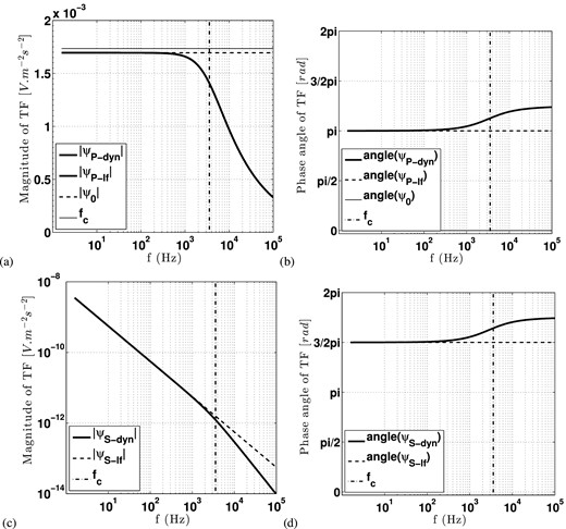
Magnitude (a) and phase angles (b) as a function of the frequency f, respectively for the P-waves dynamic transfer function ψP-dyn, for the P-waves low frequency transfer function ψP-lf and for the P-waves simplified low frequency transfer function ψ0 in a saturated sand (formulation in Appendix A and physical parameters in Table 1). Panels (c) and (d) are the magnitudes and phase angles of the S-waves transfer functions (ψS-dyn and ψS-lf) for the same parameters of the computations shown in (a) and (b). The Biot's frequency fc is shown with a vertical dashed line on all graphs.
Definition and values of the physical parameters involved in the computations of the transfer functions in a water saturated silica sand.
| Physical parameter | Notation | Value | Units | |
|---|---|---|---|---|
| Fluid | ||||
| Density | ρf | 103 | kg m−3 | |
| Dynamic viscosity | ηf | 10−3 | Pa s | |
| Elastic modulus | Kf | 2.5 × 10⁹ | Pa | |
| Electrical conductivity | σf | 1.17 × 10⁻² | S m−1 | Measured |
| Solid (silica sand grains) | ||||
| Grain density | ρs | 2.65 × 10³ | kg m−3 | |
| Elastic modulus | Ks | 3.6 × 10¹⁰ | Pa | |
| Porous medium | ||||
| Porosity | ϕ | 0.4 | Measured | |
| Intrinsic permeability | k0 | 1.02 × 10⁻¹¹ | m2 | Measured |
| Tortuosity | γ0 | 1.75 | From Berryman (1981) | |
| Drained or frame modulus | KD | 2.5 × 10⁷ | Pa | From seismic velocities |
| Shear frame modulus | G | 1.54 × 10⁷ | Pa | |
| Pore space term | m | 6 | From Pride (1994) | |
| Electrokinetic coefficient | Cek | −1.73 × 10⁻⁶ | V Pa−1 | From Guichet et al. (2003), see Appendix B |
The main information in Fig. 1 is that the predicted |$| \mathbf {E}_{{\rm S}}/ \mathbf {\ddot{U}}_{{\rm S}} |$| ratios are tiny compared to the |$| \mathbf {E}_{{\rm P}}/\mathbf {\ddot{U}}_{{\rm P}}|$| (factor at most 10−6 between those two ratios). Even if the measurements of a seismoelectric field in a transverse direction compared to the main longitudinal P-wave direction may be of interest, the analysis of such small transfer functions in S waves seems out of reach both numerically and experimentally as already foreseen by Garambois & Dietrich (2001). Note also that as indicated by eq. (11), the coseismic seismoelectric fields associated to P and S waves are phase shifted by an angle π/2 as seen in Figs 1(b) and (d). We conclude that the global ratio |$| \mathbf {E}/\mathbf {\ddot{U}}|$| is useless as soon as P and S waves coexist in the seismic signal, since only the P waves are efficiently converted into electric field: the magnitude of the ratio |$| \mathbf {E}/\mathbf {\ddot{U}}|$| is shifted towards smaller values compared to the analytical P transfer function ψP-dyn when S waves are present.
Computations in Fig. 1 confirm that the low frequency approximations ψP-lf and ψS-lf are consistent with the dynamic transfer functions ψP-dyn and ψS-dyn as long as the current frequency is below the Biot's frequency (Garambois & Dietrich 2001). This behaviour is in good agreement with experimental measurements of frequency dependent coupling coefficients (Reppert et al.2001; Tardif et al.2011). For f ≫ fc, the magnitude of the dynamic transfer function for P waves strongly decreases as the frequency increases. It is also worth to notice in Figs 1(a) and (b) that although the computation for f ≪ fc of the simplified low frequency transfer function ψ0 gives a correct magnitude (within 3 percents) compared to ψP-dyn or ψP-lf formulations, ψ0 is phase shifted by π compared to ψP-dyn or ψP-lf. As a consequence, the seismoelectric signals predicted by the simplified low frequency transfer function ψ0 have to be used cautiously since it may lead to some misinterpretations regarding the polarity of the seismic signal compared to electrical signal.
2.2 The effective fluid model
The theoretical transfer functions shown in Section 2.1 were developed for fluid-filled porous media since they were based on the original Biot's formulation. However, partial saturation has a strong impact on both seismic propagation and electrokinetic coupling. As long as the seismic wavelengths are much larger than the fluid heterogeneities, the simplest way to account for this partial saturation is to use effective fluid models as basically performed in seismic surveys (Bachrach & Nur 1998) or laboratory measurements (Barrière et al.2012).
For this purpose, the terms ρf, ρ, C, H, σf and Cek in eqs (3), (4) (dynamic formulation) and (11) (low frequency formulation) are replaced by their effective values depending on the water saturation Sw (defined as the pore volume ratio filled with water). The details of this classic effective model are given in Appendix A. Several models of electrokinetic coefficient Cek(Sw) accounting for partial saturation were constructed from theoretical studies and/or laboratory measurements (Guichet et al.2003; Darnet & Marquis 2004; Revil & Cerepi 2004; Revil et al.2007; Allègre et al.2010, 2012; Jackson 2010). The Biot frequency ωc is therefore strongly affected via its dependence on ρf(Sw) and ηf(Sw). The various Cek(Sw) models used in this study are described in Appendix B; all the electrokinetic models can be written under the following expression Cek(Sw) = Cek(Sw = 1)f(Sw) where f(Sw) are listed in Table 2 for the different models. The way we have derived the saturated value of Cek(Sw = 1) is also detailed in Appendix B.
List of the various functions f(Sw) used in the electrokinetic coefficient depending on saturation Cek(Sw) = Cek(Sw = 1)f(Sw). The various used notations are detailed in Appendix B.
| Model | f(Sw) | Reference |
|---|---|---|
| Linear model | Se | Guichet et al. (2003) |
| Volume averaging | |$S_e ^{\frac{2+3\lambda }{\lambda }}/S_{\rm w} ^{n+1}$| | Revil et al. (2007) |
| Capillary tubes | |${S_e}/{S_{\rm w} ^n}$| | Jackson (2010) |
Computations of the Cek(Sw) models presented in Fig. 2 in the Sw = [0.2 − 1] range show that, using the parameters of our experiment, two main trends are expected: Guichet et al. (2003) and Revil et al. (2007) models predict an increase of Cek(Sw) when Sw increases, whereas Jackson (2010) model predicts the opposite behaviour. Indeed, the choice of the electrokinetic model Cek(Sw) is rather important since Cek amplitudes can vary by a factor of ten between various models in the considered saturation range.
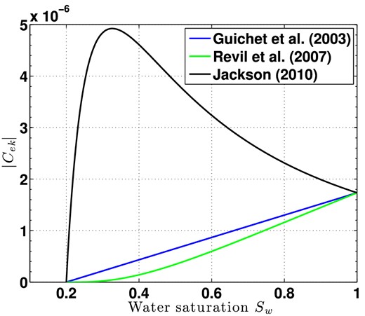
Absolute values of the coupling electrokinetic coefficients ∣Cek(Sw)∣ as a function of the water saturation Sw, for different electrokinetic models. The analytical formulations of the models are shown explicitly in Appendix B.
We will discuss in the following the effect of water saturation on seismoelectric transfer functions amplitudes. Since the use of all these models at once would make our discussion more complex, we propose to use the model of Jackson (2010), |$C_{{\rm ek}}(S_{\rm w}) = C_{{\rm ek}}(S_{{\rm w}} = 1) S_{\rm e} S_{\rm w} ^{-n}$|, as a reference, since it predicts values close to the experimental measurements presented in Section 4.
2.3 Seismoelectric transfer functions in partially saturated sands
We have presented in Section 2.1 both the dynamic and low frequency transfer functions in a fluid-filled silica sand. We have used the effective properties of the fluid and electrokinetic models to rewrite key terms depending on the water saturation in Section 2.2. The physical parameters needed to express the transfer functions as a function of partial saturation are listed in Table 3.
Definition and values of the physical parameters involved in the computations of the transfer functions in a partially saturated silica sand. f(Sw), entering in the definition of Cek(Sw), are given in Table 2.
| Physical parameter | Notation | Value | Units | |
|---|---|---|---|---|
| Fluid (water and gas) | ||||
| Density | ρw | 103 | kg m−3 | |
| Dynamic viscosity | ηw | 10−3 | Pa s | |
| Elastic modulus | Kw | 2.5 × 10⁹ | Pa | |
| Electrical conductivity | σw | 1.17 × 10⁻² | S m−1 | Measured |
| Gas density | ρg | 1.2 | kg m−3 | |
| Dynamic viscosity | ηg | 10−5 | Pa s | |
| Elastic modulus of air | Kg | 1.5 × 10⁵ | Pa | |
| Solid (silica sand grains) | ||||
| Grain density | ρs | 2.65 × 10³ | kg m−3 | |
| Elastic modulus | Ks | 3.6 × 10¹⁰ | Pa | |
| Porous medium | ||||
| Porosity | ϕ | 0.4 | Measured | |
| Intrinsic permeability | k0 | 1.02 × 10⁻¹¹ | m2 | Measured |
| Tortuosity | γ0 | 1.75 | From Berryman (1981) | |
| Drained or frame modulus | KD | 2.5 × 10⁷ | Pa | From Walton (1987), checked on seismic velocities |
| Shear frame modulus | G | 1.54 × 10⁷ | Pa | |
| Electrokinetic coefficient | Cek(Sw) | −1.73 × 10⁻⁶ × f(Sw) | V Pa−1 | From Guichet et al. (2003), see Appendix B |
| Residual water saturation | Sw0 | 0.2 | ||
| Pore space term | m | 6 | From Pride (1994) | |
| Second exponent of Archie's law | n | 2.58 | From Doussan & Ruy (2009) | |
| Curve shape parameter | λ | 1.7 | From Revil et al. (2007) |
Using the hypotheses of the calculation detailed in Appendix A, Fig. 3 presents magnitudes and phase angles of the partial saturation transfer function ψP-dyn(Sw, ω), ψP-lf(Sw), ψ0(Sw) as a function of the water saturation. We clearly see that the Biot's frequency (white line in Fig. 3a), varies significantly in the Sw = [0–1] range. Fig. 3(a) displays the evolution of the magnitude ∣ψP-dyn(Sw, ω)∣ in a colourmap representation as a function of the saturation and the frequency: it shows that, using the Pride's theory (1994) extended to effective fluid models with Jackson (2010) model, the magnitude of the dynamic transfer function is expected to remain rather constant in the Sw = [0.2−0.9] saturation range. Note that the choice of the Cek(Sw) model (among the ones seen in Appendix B and in Table 2) can affect the shape of the magnitude of ψP-dyn(Sw) from a clear increase to a rather constant behaviour (see the solid black, blue and green curves of Fig. 3b, respectively obtained by using Jackson 2010; Guichet et al.2003; Revil et al.2007).
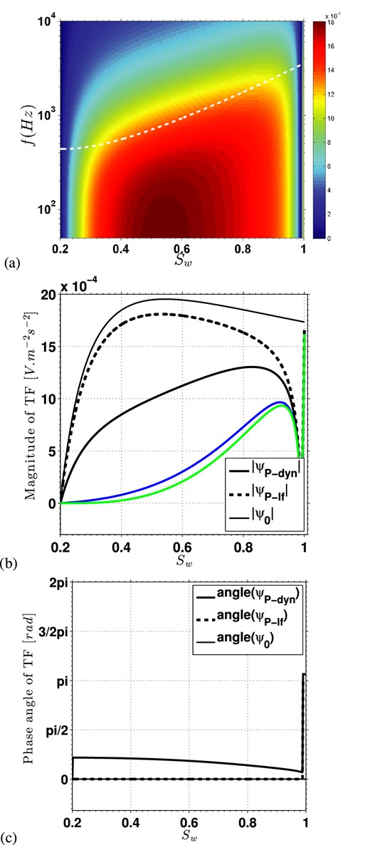
(a) Magnitude of the P-waves dynamic transfer function ∣ψP-dyn(Sw, ω)∣ as a function of frequency f and saturation Sw, based on the Jackson (2010) model for electrokinetic coupling. The white line gives Biot's frequency values as a function of Sw. (b) and (c): Magnitudes and phase angles as a function of the saturation Sw, respectively for the P-waves dynamic transfer function ψP-dyn at f = 1.5 kHz, for the P-waves low frequency transfer function ψp-lf and for the P-waves simplified low frequency transfer function ψ0 in a partially saturated silica sand. Magnitude of dynamic transfer functions obtained with the models of Guichet et al. (2003) and Revil et al. (2007) are respectively displayed by blue and green curves.
For very high saturations (close to Sw = 1), ∣ψP-dyn(Sw, ω)∣ strongly decreases towards 0 before a final increase to the value of the saturated transfer function described in Section 2.1. This effect is even better seen in Figs 3(b) and (c) which shows the magnitudes and phase angles of the transfer functions ψP-dyn, ψP-lf, ψ0 at a particular frequency f = 1.5 kHz (close to the experimental measurements presented in Section 3). Minimum values of ∣ψP-dyn∣ and ∣ψP-lf∣ in Fig. 3(b) corresponds to the specific saturation (Sw ≃ 0.99) where important changes occur in the transfer function close to Sw = 1, originating from strong changes in the poroelastic moduli KU, H and C (Bachrach & Nur 1998). Since the term involving the poroelastic moduli contribution was neglected in the expression of the simplified low frequency transfer function ψ0 (see eq. 7), ψ0(Sw) does not quite follow the amplitudes of the complete expression ψdyn(Sw), leading to the conclusion that ψ0 should not be used in partially saturated media.
The low frequency transfer function ψ0(Sw) is expected to increase rapidly in the Sw = [0.2−0.3] range whereas ψdyn(Sw) increases more gradually. Eventually, dynamical effect at 1.5 kHz are expected to be very strong [i.e. ψP-dyn ≫ ψ0(Sw)] in the Sw = [0.3−0.8] since the considered frequency is higher than the Biot frequency (Fig. 3a).
In order to summarize Section 2, the computations performed for a silica sand indicate that:
The predicted |$|\mathbf {E}_{i}/\mathbf {\ddot{U}}_{i} |$| ratios are at least 106 times higher for P waves than for S waves. We then conclude with two points: (1) the S waves being converted very poorly into electric field, it is hopeless both numerically and experimentally to work with an S-wave seismoelectric field; (2) if one wants to use quantitatively the amplitude of transfer P-waves functions ψP-dyn, the seismic signal should be purely composed of P waves otherwise the measured magnitude |$| \mathbf {E_{P}}/\mathbf {\ddot{U}_{P}}|$| would be underestimated.
Using the Jackson (2010) model for electrokinetic coupling, the theoretically predicted |$| \mathbf {E_P}(S_{{\rm w}},\omega )/\mathbf {\ddot{U}_P}(S_{{\rm w}},\omega ) |$| does not vary significantly in the saturation range Sw = [0.2–0.9].
Working in the kiloHertz range, low frequency approximation may overestimate |$|\mathbf {E}_{P}/\mathbf {\ddot{U}}_{P}|$| ratios especially for saturations close to Sw = 0.4.
In the next section of the paper, we present a laboratory experiment designed to record seismoelectric data during variations of water saturation. The goal of this experiment is to address the question of the validity of the transfer functions by comparing measured |$|\mathbf {E_{P}}/\mathbf {\ddot{U}_{P}} |$| ratio to theoretical predictions.
3 EXPERIMENTAL SET-UP
3.1 Description of the experimental set-up
Our experimental apparatus (Barrière et al.2012) described below was built to measure seismic and coseismic fields for various water content in a very permeable and homogeneous medium. A necessary condition to observe properly the propagation of direct P waves is to get at least several wavelengths along the sample length. The porous medium is a sand extracted from a sandpit located in the Landes forest (South West of France), composed of 99 per cent of quartz, which main grain size is around 250 μm). The very low seismic velocities in uncompacted sand involve short wavelengths that enable to built reasonably sized experiments (1-m length-scale container).
The final device shown in Fig. 4 was composed of:
A wood container filled with uncompacted sand (34 cm × 35 cm × 107 cm) which bottom and lateral edges were covered by acoustic foam (Strasonic foam, Paulstra) to attenuate refracted and reflected seismic waves.
Five wells consisting of unperforated PVC pipes: imbibition was performed by injecting water under the effect of gravity through the lower extremity of wells marked by blue arrows in Fig. 4 whereas drainage was performed by pumping water through the wells marked with red arrows.
An acoustic source (pendulum) consisting in a stainless steel ball hitting a granite cylinder in contact with the sand. An accelerometer placed on the granite cylinder recorded the source signal: the obtained broad-band spectrum lies in the [0.005–20] kHz frequency range (see Figs 4b and c). This seismic source was designed to generate mainly P waves along the x-axis (Sénéchal et al.2010).
Nine single component accelerometers (IEPE type, Bruel and Kjaer) with a 50 mV (m s−2)−1 sensitivity in the [0–17] kHz range. The accelerometers were aligned with the axis of the granite cylinder and placed in the same direction to obtain a null angle of incidence for the direct P waves (x direction). They were placed every 10 cm, starting from 20 cm to 100 cm from the source. The accelerometers were oriented in order to get a negative polarity first arrival in acceleration |$\mathbf {\ddot{U}}$|, corresponding to a positive scalar product between wave vector and local displacement U (see eq. 1).
- Eight electric dipoles, composed of two stainless steel electrodes (7 cm long) and their home-made pre-amplifiers (input impedance 1 GΩ) used for the seismoelectric acquisition. The dipole line (x direction) is in the direction of the accelerometer line but translated by 1 cm laterally (see Fig. 4). The 10-cm-length dipoles were placed every 10 cm from 20 to 90 cm from the source. Since the negative electrode (by convention in our set-up) is located further from the source (the spatial reference) than the positive electrode, the measured difference in electrical potential is −ΔVx and Δx = 10 cm. The seismoelectric field is deduced from this measurement by the relation:(12)\begin{equation} E_x = -\frac{\Delta V_x}{\Delta x}. \end{equation}
Six calibrated capacitance probes (Waterscout SM 100 soil moisture sensor from Spectrum technologies) were used to monitor the water saturation Sw in the plane where accelerometers and dipoles were located. The water saturation uncertainty was evaluated to 5 per cent and the Sw value around each accelerometer or dipole was obtained by interpolation of probe measurements using the Inverse Distance Weightering method (Barrière et al.2012). The uniform saturation along the receivers line is shown in Fig. 5).
Dynamic signal acquisition modules PXI-4498 from National Instruments with 16 simultaneous 24-bit analog inputs per module (316 mV full scale for electrical potential measurements). A 200 kHz sampling rate was used.
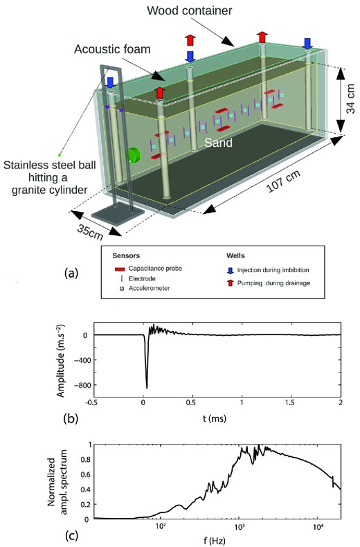
(a) Sketch of the experimental apparatus used in this study. (b) Typical record of the seismic source signal (steel ball hitting the granite) versus time, recorded by an accelerometer located on the granite cylinder. (c) Normalized amplitude spectrum of the source signal shown in (b) as a function of frequency.

Example of water saturation measurements along the receivers array for different values of Sw. Variations of Sw between offset = 0.2 and 0.4 m are lower than uncertainties on Sw measurements displayed as an example at offset = 0.3 m, during D3, when Sw is close to 0.6.
3.2 Description of the experimental constraints and parameters
Before starting an experiment, we took care to bring the saturating fluid at electrochemical equilibrium by flowing deionized water through the sand during 48 hr. The water conductivity reached a plateau value around 1.17 × 10⁻² S m−1 at 25 °C, and the monitoring during the following experiments showed it to be very stable. In this study, we have neglected the surface electrical conductivity (see Appendix A) in particular because it is generally admitted to be lower than 2 × 10⁻⁴ S m−1 for silica as long as the water conductivity remains about 10−2 S m−1 (Glover 1998; Guichet et al.2003).
The oven-dried sand were poured in the container with constant flow by using a large sieve. At the end of the experiment, five cores were extracted from the sample in order to measure their porosity and intrinsic permeability. Permeability was measured by a home made Darcy's apparatus and was estimated to k0 = 1.02 × 10⁻¹¹ m2. The porosity ϕ = 0.4 ± 0.02 was measured by comparing the weight of dried cores to the density of solid grains. Using the Archie's law, we also verified by laboratory measurements that the formation factor F = ϕ/γ0 is close to 4.3 consistently with the γ0 value obtained by the formulation of Berryman (1981).
Injection pressure was obtained by uplifting water containers 40 cm above the tank. Two initial complete cycles were performed to homogenize pore fluid distribution: the first imbibition started from oven-dried sand and was followed by a first drainage and a second complete cycle. During the last cycle, water saturation variations showed that the saturation could be considered as spatially homogeneous in the horizontal plane of measurements (Fig. 5).
We explored the Sw = [0.2–0.9] range corresponding to respectively the water and gas residual saturations. We performed a time-lapse monitoring while the saturation was varying, by repeating about 25 times (between Sw = 0.2 and Sw = 0.9) a measurement of an initial saturation measurement followed by 10 seismic/seismoelectric records and a final measurement of the saturation. For each saturation value, the ten seismic and ten seismoelectric records were stacked in order to improve the signal-to-noise ratio.
3.3 Example of measured seismic and seismoelectric data
An example of seismic and seismoelectric data recorded at the beginning of the third drainage (Sw ≃ 0.9) is presented in Fig. 6 for various offsets. An offset is defined as the distance between the source and the receiver (the accelerometer or the first electrode). It appears from the comparison of Figs 6(c) and (d) that, as expected, seismoelectric data are very sensitive to electromagnetic ambient noise. For each recorded signal, the signal-to-noise ratio (Figs 6e and f) is computed as S/N = 10 log (Asig/Anoise)2, the amplitude of the signal Asig being defined as its maximum value during the first 10 ms after triggering, and the noise amplitude Anoise being defined as the maximum value of the data before triggering.
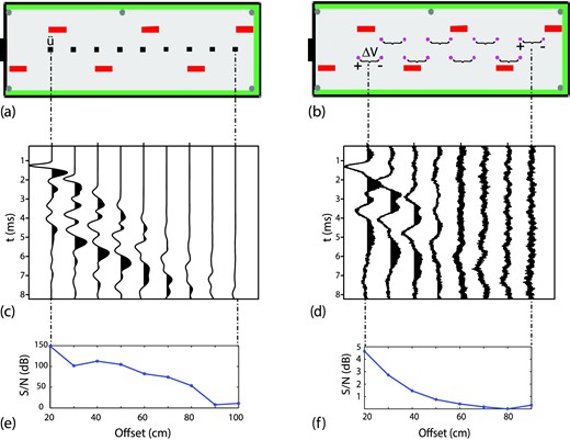
(a) View from above of the horizontal plane of the experimental set-up containing accelerometers (black squares) and capacitance probes (red rectangles). (b) View from above of the same horizontal plane shown in (a) containing dipoles (couple of electrodes in magenta). (c) Seismic records at various offsets (source–receiver distance) obtained at the beginning of the drainage of the third cycle for Sw ≈ 0.9. (d) Seismoelectric record at various offsets recorded simultaneously to the seismic data shown in (c). (e) Signal-to-noise ratio of the data shown in (c) versus offsets. (f) Signal-to-noise ratio of the data shown in (d) versus offsets.
All seismic records contain classically different types of seismic waves corresponding to direct, reflected and/or refracted waves. The seismic record in Fig. 6(c) shows fortunately very clear first arrivals up to an offset of 80 cm, with S/N higher than 100 dB as shown in Fig. 6(e). As claimed in Barrière et al. (2012), these first seismic arrivals were considered as direct P waves. The very low S/N measured on seismoelectric data (lower than 5 dB in Fig. 6f) implies that waveforms were much more difficult to identify than in seismic signals. The first seismoelectric wave-type signal could indeed be clearly distinguished only on the three first records (offsets 20, 30 and 40 cm) in Fig. 6(d).
We notice in Fig. 6(c) that the first seismic arrivals have a negative polarity consistently with what was expected from the accelerometers specifications (see Section 3.1). The measured coseismic electric field in Fig. 6(d) also presents a first negative signal implying that the corresponding |$\mathbf {E}/\mathbf {\ddot{U}}$| ratio is positive for the direct P-waves propagating in the partially saturated sand, which is consistent with the theoretical predictions developed in Section 2.3 (see Fig. 3 with a phase angle near zero for ψP).
The recorded seismic and seismoelectric signals during the third drainage (Sw decreasing from 0.88 to 0.24) at offset = 20 cm are shown in Fig. 7. In Fig. 7(a), seismic and seismoelectric traces are normalized in order to perform a qualitative comparison of both signals during first arrivals. It appears clearly that the frequency content of seismic and seismoelectric signals are rather different. This observation calls for the use of a time-frequency analysis in order to characterize seismic and seismoelectric attributes. We proceed the data in the following by using a CWT which in turn will provide amplitudes, frequencies and velocities from the first arrival of seismic and seismoelectric measurements.
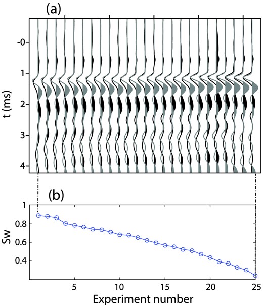
(a) Normalized seismic traces (grey) and seismoelectric fields (black) measured at offset = 0.2 m during the third drainage. (b) Sw coefficient as a function of the experiment number shown in (a).
4 ANALYSIS OF FIRST SEISMIC AND SEISMOELECTRIC ARRIVALS
We have presented in Section 2 an analytical formulation of the transfer function giving the amplitudes of seismoelectric fields induced by a seismic wave travelling in a porous medium. These transfer functions were given in particular for P and S direct body waves. Barrière et al. (2012) performed a 2-D numerical simulation of waves propagation in the present experiment and showed that the first arrivals as shown in Fig. 6(c) were indeed direct P waves, not disturbed by reflected, refracted nor surface waves.
In order to analyse the frequency content of these first P-waves arrivals, we chose to perform a spectral analysis on the first envelope or ‘lobe’ by using a CWT (Daubechies 1992; Mallat & Zhong 1992). This processing is detailed in Section B3. From typical C(a, b) map obtained by CWT, we can extract the following informations concerning the first arrivals:
The main frequency of the first arrival, by picking the scale corresponding to the maximum of C(a, b). The picked scale in Fig. B1(b) was converted in frequency using eq. (B6). The function converting scales into frequencies is shown in Fig. B1(c). The local spectrum can also be estimated from CWT by extracting local maxima in the time window corresponding to the first arrival (highlighted band in Fig. B1b).
The time at the maximum of C(a, b) in a time window corresponding to the first arrival. From that time we will deduce the propagation time of the first arrival, by substracting a quarter period corresponding to the main frequency.
The amplitude of the first arrival by picking the maximum amplitude of the wavelet coefficient in the C(a, b) map.
The CWT using a Mexican hat wavelet, shown as an example here, was performed on all seismic and seismoelectric data sets. We focus in the following on the results of cycle 3 (imbibition and drainage written respectively, I3 and D3).
4.1 Seismic and seismoelectric velocities
The apparent velocity of seismic and seismoelectric fields are deduced from the analysis of C(a, b) maps. We picked the main frequency (see Section 4.2) and the corresponding time for all measurements, and then substracted to that picked time a quarter period at the main frequency in order to get a precise estimation of the absolute ‘first break’ time. For a given experiment, this time determination is performed for all offsets. The apparent velocity for seismic and seismoelectric data is then deduced by a linear regression of all these first break times versus distances. Only the first three positions (offsets) were used since the seismoelectric data became too noisy after offset 0.4 m. We found that the described apparent velocity determination technique was well suited for seismoelectric measurements which first breaks were not always very clear in the raw data (see for example Fig. 6e).
A compilation of seismic and seismoelectric apparent velocities measured during the third cycle is shown in Fig. 8 as a function of saturation Sw. At first order, a rather constant mean apparent velocity for seismic and seismoelectric fields was found lower than 200 m s−1 (between 140 and 180 m s−1) during both drainage and imbibition. Nearly identical velocities in seismic and in seismoelectric demonstrates the expected coseismic origin of the seismoelectric data measured experimentally.
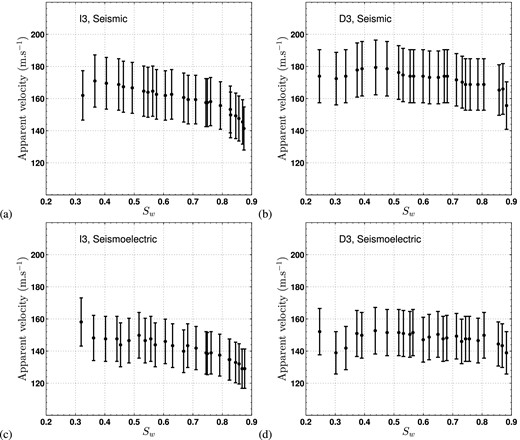
Apparent seismic and seismoelectric velocities measured during the third cycle as a function of Sw. (a), (b), (c) and (d) are respectively the seismic velocities during imbibition (I3), seismic velocities during drainage (D3), seismoelectric velocities during imbibition and seismoelectric velocities during drainage. The error bars, around 10 per cent of the measured velocity, originate from uncertainties on the accelerometers locations (±5 mm), on the picking times (±4 × 10⁻⁵ s) and on the dipole lengths between coupled electrodes (±10 mm).
Barrière et al. (2012) monitored the phase velocity during imbibition and drainage also in the CWT domain by using a complex ‘Morlet’ instead of a real ‘Mexican hat’ wavelet used in this study. The method consisted in picking time shifts both in amplitude and in phase spectra, and in deducing the corresponding phase velocity. Here, our simplified procedure using a real ‘Mexican hat’ wavelet, chosen because it appears the more adapted to describe the studied first lobe of the signal, gave results comparable to those of Barrière et al. (2012) in terms of velocity values of the direct P waves.
4.2 Frequency content of seismic and seismoelectric fields
Main frequencies obtained by CWT in seismic and seismoelectric data during the third cycle are presented in Fig. 9. The first observation is that main frequencies globally decrease as a function of an increasing offset, either in seismic or in seismoelectric fields: that is understood as a classic attenuation effect of the higher frequencies. A second common characteristic in seismic and seismoelectric frequencies (Figs 9a–d) is a decrease of frequencies as a function of an increasing water saturation Sw. That trend, already observed by Barriere (2011) in a purely seismic context, was attributed to Biot's losses attenuation combined to effective permeability effects.
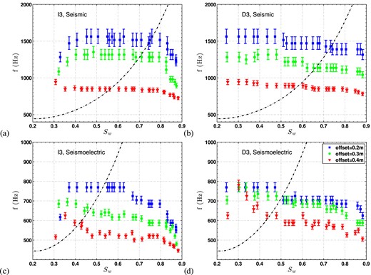
Main frequency (picked from a CWT signal processing) obtained during the third cycle from respectively (a) the seismic data during imbibition, (b) the seismic data during drainage, (c) the seismoeletric data during imbibition and (d) seismoelectric data during drainage. All figures are shown as a function of the saturation Sw and for three different offsets: blue squares 0.2 m, green circles 0.3 m and red triangles 0.4 m. The error bars originate from uncertainties in picking pseudo frequencies (± 2 samples around the maximum amplitude). The variations in Biot's frequency versus saturation (computed from eq. 5 and Appendix A) during those experiments are shown with a dashed black line.
It appears systematically in Fig. 9 that for a given water saturation, the main frequency of the first seismic lobe is higher than the counterpart seismoelectric first lobe frequency; seismic frequencies remain for example always about twice higher than the seismoelectric frequencies at offset 0.2 m. These gaps in frequency cannot be explained by the low frequency transfer functions (ψ0 and ψP-lf) since the latter assume that seismic and seismoelectric signals are linearly dependent in time and frequency (see eq. A8 in Appendix A). In other words, the low frequency transfer function derived from Pride's model extended to the effective fluid presented in Section 2.2 can not account for all the seismic and seismoelectric main frequencies discrepancies observed in Fig. 9, especially when the measured frequency is lower than the Biot's frequency (correspond in Fig. 9 to Sw ≳ 0.6). Some data in Fig. 9 are well above the Biot's frequency and dynamic effect are probably coming into play in the transfer function between seismic and seismoelectric fields. At least qualitatively, we may infer from Fig. 9 that the frequency content would be modified when the measured frequency crosses the Biot's frequency, corresponding to changes in attenuation mechanisms (inertial or viscous flows).
Computations performed in Section 2.2 showed that we expect a decrease of the magnitude of the ratio |$| \mathbf {E}/\mathbf {\ddot{U}}|$| as a function of the frequency, for a given Sw, when the main seismic frequency exceeds the Biot's frequency (follow a vertical direction in Fig. 3a for a given Sw). More precisely, we estimate from these computations that ∣ψP-dyn(0.6 kHz)∣/∣ψP-lf∣ ≃ 0.85 when ∣ψP-dyn(1.5 kHz)∣/∣ψP-lf∣ ≃ 0.55 for Sw = 0.6: we then expect experimentally the magnitude of the transfer function ∣ψP-dyn∣ to decrease for f above the Biot's frequency (at a given Sw), meaning that the seismic amplitudes at a given frequency should decrease less rapidly than the seismoelectric amplitudes at that same frequency. We can not conclude in Fig. 9 if this trend is observed since only the main frequencies are shown and that seismic and seismoelectric main frequencies do not overlap; we will discuss this point further in Section 4.3.
The strong difference in dominating frequency between seismic and seismoelectric signals mentioned above is a quite common observation in laboratory measurements (Zhu & Toksöz 2003; Bordes et al.2006, 2008) as well as in seismoelectric surveys, even at seismic frequencies much lower than the Biot's frequency (Strahser et al.2007; Dupuis et al.2009). Since large dipoles are strongly disturbed by electromagnetic noise, authors generally try to reach a compromise by improving the signal-to-noise ratio (Garambois 1999). Some preliminary tests showed in our case that a 10 cm dipole length was a suitable distance between electrodes, giving satisfying signal-to-noise ratio. Nevertheless, seismic signals, obtained with a calibrated and localized sensor, can be directly interpreted as local acceleration whereas seismoelectric measurements are indirect since they are obtained by a dipole. To our knowledge, the role of the acquisition geometry was never discussed so far, and we suspect that the dipole length might have an effect on the frequency content of the seismoelectric signal. A better understanding of the frequency mismatch between seismic and seismoelectric would require a more complete experimental and/or numerical study addressing the effect of acquisition geometry on seismoelectric frequency content which was not our initial purpose.
4.3 Amplitudes ratios
The maximum amplitude of the first arrival in seismic and seismoelectric experiments during cycle 3 are shown in Fig. 10. These amplitudes were directly extracted from the signal in time by picking the maximum of the first lobe. As expected, measured amplitudes decrease as a function of offset and decrease also as a function of water saturation in the range Sw = [0.2−0.9], consistently with previous observations of Parkhomenko & Tsze-San (1964) for seismoelectric measurements and Barrière et al. (2012) for seismic measurements. These absolute amplitudes can not be however directly interpreted in term of seismoelectric coupling since, for example, the seismic amplitudes strongly depend on seismic attenuation. That is why the transfer functions built upon a ratio of a coseismic to a seismic field, can precisely be seen as a direct measurement of seismoelectric coupling.

First arrival amplitude (picked in time signals) during the third cycle from, respectively (a) the seismic data during imbibition, (b) the seismic data during drainage, (c) the seismoeletric data during imbibition and (d) seismoelectric data during drainage. All figures are shown as a function of the saturation Sw and for three different offsets: blue squares 0.2 m, green circles 0.3 m and red triangles 0.4 m. The associated error bars (around 7 per cent) in seismic and seismoelectric amplitudes originate from uncertainties in the receivers location (±5 mm), in the dipole length (±10 mm) and on the picking of the maximum amplitude (±2 samples around the maximum amplitude).
In order to derive experimental transfer functions from our data, we start with a ‘static’ approach consisting in directly computing the ratio of the seismoelectric to seismic maximum amplitudes: this procedure assumes that the transfer function does not depend on frequency although measured seismic and seismoelectric main frequencies are significantly different (see Section 4.2). These ratio |$| \mathbf {E}/\mathbf {\ddot{U}} |_{{\rm exp}}$| are presented in Fig. 11 for the experiments performed during the third cycle. We have obtained these ratio by two independent ways: the first technique called ‘Time-static’ in Figs 11(a) and (b) is obtained from the data picked in time signals (shown in Fig. 10). The second technique, labelled ‘CWT-static’ in Figs 11(b) and (d), consists in picking the amplitudes of the first arrival (respectively in seismoelectric and in seismic signals) associated to the main frequency obtained by CWT (see Section 4.2) and then perform the ratio.
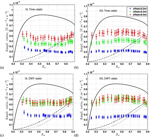
Amplitude ratios of seismoelectric to seismic field as a function of Sw measured during the imbibition of the third cycle in (a) and (c), and during the drainage of the third cycle in (b) and (d) at offset = 0.2 m (blue squares), at offset = 0.3 m (green circles) and offset = 0.4 m (red triangles). The amplitude ratios obtained in the ‘static approach’ are obtained in (a) and (b) by picking the maximum amplitude in time signals (Time-static), and in (c) and (d) by picking maximum amplitudes of seismic and seismoelectric first arrival in the C(a,b) map. The low frequency transfer function ∣ψP-lf(Sw)∣ predictions are obtained by applying an electrokinetic coefficient two times smaller compared to the theoretical Cek computed in Appendix A. They are superimposed in Fig. (a) and (b) using the model of Jackson (2010) in solid line, Guichet et al. (2003) long dashed line and Revil et al. (2007) short dashed line.
The two independent techniques of measurement of |$| \mathbf {E}/\mathbf {\ddot{U}} |_{{\rm exp}}$| lead to the same conclusion: the ratio of seismoelectric to seismic signals is at first order constant as function of the saturation Sw for a given offset in the explored range Sw = [0.2−0.9]. In terms of order of magnitude, the mean |$|\mathbf {E}/\mathbf {\ddot{U}} |_{{\rm exp}}$| is about 4 × 10⁻⁴ ± 25 per cent. Although the two techniques are rather different, one processing the data in the time domain and the other one in the CWT, the differences in the ratios remain as small as ∼10–25 per cent (comparison of Fig. 10a with Fig. 11c, and Fig. 11 with Fig. 11d).
These results can also be compared to the theoretical transfer function discussed in Section 2.3. The continuous and dashed lines in Fig. 11 are obtained by computing the ∣ψP-lf(Sw)∣ with the three electrokinetics models presented in Table 2. Nevertheless, the models are computed by considering an electrokinetic coefficient two times smaller compared to the theoretical Cek computed in Appendix A, which were based on the Cek(Sw) = 1 values measured by Guichet et al. (2003) [here we use Cek(Sw = 1)/2]. It appears from Fig. 11 that amplitude ratios as a function of the saturation are well reproduced by the capillary tubes model of Jackson (2010) (plateau) whereas the increase predicted by Guichet et al. (2003) and Revil et al. (2007) is not retrieved in the data.
The comparison of an ‘experimental transfer function’ with the dynamical transfer functions predictions seen in Section 2 would require to perform spectra ratios on a broad-band frequency range; the analysis of both amplitude and phase of spectra ratios could lead to a discussion on the validity of the dynamic transfer function. Unfortunately, in the present experiment, the explored frequency range is too narrow and such a complete analysis is out of reach. An alternative approach consists in calculating amplitude ratios extracted from the C(a, b) maps at the main frequency or at a frequency in the vicinity of the main frequency. The ‘dynamic’ approach consists in picking the maximum amplitude at the main frequency in seismoelectric data (shown in Figs 10c and d), and, thereafter, in picking the counterpart seismic amplitude at that same seismoelectric main frequency (denoted SEMF, ‘SeismoElectric Main Frequency’) in the C(a, b) maps. We then perform the ratio between those amplitudes for all experiments at various saturation and obtain the results in Fig. 12. Similarly to the ‘static’ approach shown in Fig. 11, it results that those ratios, for a given offset, are nearly constant as a function of saturation with a mean value 5 × 10⁻⁴ ± 25 per cent. The data in Fig. 12 can be compared to the theoretical prediction of the dynamical transfer function ∣ψP-dyn(Sw)∣ using the Jackson (2010) model with an electrokinetic coefficient equal to Cek(Sw = 1)/2. Since the working frequencies in the experiments are close to the Biot's frequency, as discussed in Section 2.3, the theoretical dynamical transfer functions are significantly different in amplitudes compared to static ones: the dynamic transfer functions are closer to the data than the static ones.
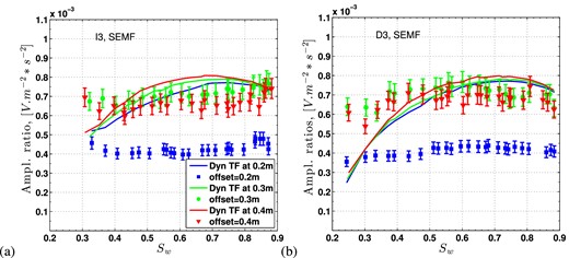
Amplitude ratios of seismoelectric to seismic field as a function of Sw measured during the imbibition (a) and drainage (b) of the third cycle. These data are obtained with the ‘dynamic approach’ by picking the maximum amplitude at the main frequency of seismoelectric data, and, thereafter, by picking the counterpart seismic amplitude at that same seismoelectric main frequency (denoted SEMF, ‘SeismoElectric Main Frequency’) in local maxima curve of the C(a, b) maps. Dynamic transfer functions are also computed at the observed frequency for each offset, using the Jackson (2010) model with an electrokinetic coefficient two times smaller compared to the theoretical Cek computed in Appendix A.
Our ‘static’ and ‘dynamic’ approaches of the experimental data demonstrate that for given offset, the ratio |$| \mathbf {E}/\mathbf {\ddot{U}}| _{{\rm exp}}$| remain nearly constant during the experiments even if the range of variation Sw = [0.2−0.9] is quite large. This global trend is particularly well recovered by the Jackson's model (2010) coupled to the extended theory of Pride (1994) to a partially saturated fluid. More quantitatively, there is however a mismatch in terms of amplitude of the ratio |$| \mathbf {E}/\mathbf {\ddot{U}}|$|: the theoretical predictions are systematically much lower than the experimental data, about a factor 4 when the static approach is used and about a factor 2 when the dynamic approach is used. This mismatch could originate from an overestimation of electrokinetic coefficient Cek (see Appendix B) or from our choice of dipole length. Indeed, we observe that the dipole length can modify the amplitude of the measured E field by a coefficient ranging 1.5–4, but not depending on the saturation.
5 CONCLUSION
Pride & Haartsen (1996) wrote the expressions of transfer functions from seismic to seismoelectric fields in a saturated porous medium. Later, Garambois & Dietrich (2001) proposed a simplified low frequency transfer function applicable when seismic frequencies are below Biot's frequency. Both studies were performed in a saturated porous media. We have generalized the transfer functions formulations to a partially saturated porous medium and have consequently derived analytical expressions of dynamic and low frequency transfer functions for P and S waves, respectively ψP-dyn(Sw, ω), ψP-lf(Sw) and ψS-dyn(Sw, ω), ψS-lf(Sw, ω). The generalization to partially saturated medium was done using an effective fluid model under various hypotheses; we have in particular neglected the surface conductivities and used characteristic models of variations of the electrokinetic coupling Cek as a function of the partial saturation Sw. In this study, we have particularly emphasized the model proposed by Jackson (2010). The effective fluid model also assumes that the seismic wavelengths are larger that the fluid heterogeneities.
The theoretical P-waves transfer functions showed significant variations in magnitude versus saturation and versus frequency. For a given frequency, the magnitude ∣ψP-dyn(Sw)∣ increases in the typical range Sw = [0.2–0.4] but is predicted to be nearly constant in the Sw = [0.4–0.9] range. For a given saturation, ∣ψP-dyn(f)∣ versus frequency is firstly constant before rapidly decreasing once we exceed Biot's frequency. The variation of ∣ψP-dyn(Sw, ω)∣ is of the order 10 in the considered range (Sw = [0.2–0.9], f = [10–104] Hz) and depends both on the used model for Cek(Sw) and on the chosen frequency. We have also shown numerically that the magnitude of the P-waves low frequency transfer functions follows closely the dynamic one when f ≤ fc. We also showed that the low frequency transfer function may be carefully simplified in partially saturated media since excessive simplification introduces errors on phase predictions at highest saturations. Finally, we confirmed that the transfer function of the shear S waves is tiny compared to the P-waves case; we concluded that the S-waves transfer functions may not be used either in experimental or numerical conditions.
We have then compared our theoretical predictions to data recorded in a partially saturated tank of silica sand: Sw was monitored during experiments (drainage and imbibition), the seismic field was recorded using accelerometers while the seismoelectric field was recorded using a couple of electrodes at mid-height of the 1-m-length-scale container. We have shown using the CWT that the seismic field had systematically a main frequency about twice as big as the main seismoelectric frequency; that observation was true for all offsets (distance to the source).
We have also estimated the experimental ratios |$|{{\bf E}_{P}}(S_{{\rm w}})/{{\bf \ddot{U}_{P}}}(S_{{\rm w}})|$| with various methods (picking in time and CWT) and those ratios appear to be approximatively constant during the experiments in the range Sw = [0.2–0.9] for all offsets. The comparison of data with the theory led to the conclusion that the trend and the order of magnitude of the recorded experimental transfer functions is recovered by the theoretical prediction when using the Jackson (2010) model for the saturation dependence of electrokinetic coefficient. Working near the Biot's frequency in the experiments, we verified that dynamics effects come into play since the dynamic transfer function is closer to the data than the static transfer function. We have also demonstrated that the CWT processing is well suited for estimating apparent velocities, main frequencies and amplitude ratio at the main frequency of the data.
This study confirms that introducing the effective fluid model into the Pride's theory is appropriate when wavelengths are larger than the fluid heterogeneities. Nevertheless, the accuracy of the predicted transfer function strongly depends on electrokinetic models, that have to be completed to account more precisely for the fluid distribution that can involve different fluid thicknesses with strong effects on the effective viscosity and permeability.
This study has benefited to the ANR program of the French government, especially via the TRANSEK project. The authors thanks S. Garambois, G. Sénéchal and D. Rousset for their constructive suggestions and J. Holzhauer for reading carefully the original manuscript.
REFERENCES
APPENDIX A: DYNAMIC TRANSFER FORMULATION AS A FUNCTION OF SATURATION Sw
We present the set of equations used in our analytical calculations of dynamic and low frequency transfer functions. These equations are derived from the original work of Pride (1994) and Pride & Haartsen (1996) whose formulations were written for a fluid-filled porous medium. We extend Pride's models to a partially fluid saturated medium using an effective model, the main assumption being that we are dealing with seismic waves which wavelengths are much larger than fluid heterogeneities. We follow a similar approach to what has been done in Garambois & Dietrich (2001), Barrière et al. (2012) and Warden et al. (2013).
The input parameters are defined and listed in Tables 1 and 3:
Fluid: ρw, ηw, Kw, σw, ρg, ηg, Kg,(seven parameters);
Solid: ρs, Ks,(two parameters);
Porous medium: ϕ, k0, γ0, KD, G, Cek(Sw = 1), f(Sw), m, n.(nine parameters),
where subscripts w and g, respectively, refer to water and gas. These parameters are then combined to lead to the dynamic and low frequency transfer functions for P and S waves derived below.
We neglect the surface conductivities and use a reduced version of the electrical conductivity σ(Sw) in eq. (A3) compared to a more general expression of the dynamic electrical conductivity |$ {\sigma (S_{{\rm w}},\omega ) = \frac{\phi }{\gamma _{0}}S_{{\rm w}}^{n}\sigma _{{\rm w}} + 2\frac{\phi }{\gamma _{0}}\frac{C_{{\rm em}}+C_{{\rm os}}(\omega )}{\Lambda }}$| (e.g. Warden et al.2013). Using such reduced formulation, we assume that the electromigration Cem and electroosmotic Cos conductances as defined in Pride (1994) are negligible in the calculation of the dynamic electrical conductivity, as stated in Garambois & Dietrich (2001).
We use a reduced version of the effective electrical permitivity |$\tilde{\varepsilon }$| in eq. (A4) compared to a more general dynamic expression |$\tilde{\varepsilon }(S_{{\rm w}},\omega ) \!=\! { {\varepsilon (S_{{\rm w}},\omega )\!+\!\frac{i}{\omega } \sigma (S_{{\rm w}},\omega ) \!-\! \tilde{\rho }(S_{{\rm w}},\omega )L^{2}(S_{{\rm w}},\omega ) }}$|. We assume that we remain in the low-frequency range and diffusive regime where |$\varepsilon (\omega ) \ll {\frac{i}{\omega }} \sigma (\omega )$| (Garambois & Dietrich 2001). We also neglect for consistency the electroosmotic term |$\tilde{\rho }(\omega )L^{2}(\omega )$| in the dynamic expression.
The static electro-coupling coefficient L0 in eq. (A5) is multiplied by |$ {( 1 - 2\frac{\tilde{d}}{\Lambda } )}$| in the Pride's version, where |$\tilde{d}$| is basically the electrical double-layer thickness and Λ is the pore-shape factor or nearly the radius of the pores. This pre-factor in L0 is tiny (less than a tenth of a per cent) in our case and is then neglected.
- The dynamic electro-kinetic coupling of Pride (1994) is defined aswhere δ is the skin depth. For consistency with the previous hypotheses, we have also chosen to ignore both terms in parentheses since they represent again a very tiny correction to L in eq. (A5) in the frequency band of this study.\begin{equation} L(\omega ) = L_0 \left[ 1 - {\rm i} \frac{\omega }{\omega _c} \frac{m}{4} \left( 1 - 2\frac{\tilde{d}}{\Lambda } \right)^2 \left(1-i^{3/2}\frac{\tilde{d}}{\delta (\omega )} \right)^2 \right]^{-\frac{1}{2}}, \end{equation}
APPENDIX B: Cek VALUE AS A FUNCTION OF SATURATION Sw
B1 Cek at saturation Sw = 1
Since we have not performed any zeta potential measurements here, we have also used ζ = −29 mV for our sand in saturated conditions which lead to Cek(Sw = 1) = −1.73 × 10⁻⁶ V Pa−1 (value used in Tables 1 and 3) for the conductivity of the electrolyte σw = 1.17 × 10⁻² S m−1.
B2 Cek versus Sw
We detail in the following the different models giving the dependence of Cek versus Sw as listed in Table 2.
B3 On the use of the CWT
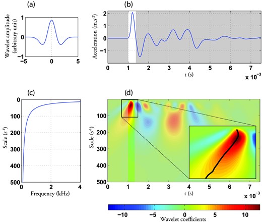
Example of a continuous wavelet transform (CWT) performed on seismic data. (a) Mother wavelet function chosen in this study: Mexican hat wavelet. (b) Seismic record versus time obtained during the third drainage. The first ‘lobe’ corresponding to the first arrival is highlighted. (c) Conversion from scale to frequency using eq. (B6) with f0 = 0.25 Hz. (d) C(a, b) spectrum map obtained by a CWT of the seismic signal shown in (b), the included figure shows the local maxima (black line) extracted to get a local spectrum. Colours indicate the amplitude of C(a, b) for a given a and b.
The computed spectrum in Fig. B1(d) strongly depends on the choice of the mother wavelet and corresponds to a smoothed and stretched approximation of a Fourier spectrum. CWT cannot achieve the high frequency resolution of a Fourier transform but it can however distinguish and characterize frequency properties of singular events in non stationary signals, like in our experimental data. The best spectral resolution is obtained by using mother wavelets with a lot of vanishing moments (i.e. oscillations) but the time resolution obeys the opposite rule (Perrier et al.1995); the choice of the mother wavelet is therefore a compromise between time and frequency resolution.
In this study, we propose to use a CWT during imbibition and drainage experiments in order to monitor the main frequencies, velocities and amplitudes of the first lobe in seismic and seismoelectric signals. We used the same wavelet for all CWT computations in order to legitimate the validity of a comparison between seismic and seismoelectric attributes.
Preliminary signal processing tests led to the conclusion that the real ‘Mexican hat’ wavelet shown in Fig. B1(a) was the most convenient wavelet to characterize in frequency the first lobe of the signal. The Mexican hat wavelet, defined as the second derivative of the gaussian function, is widely used in geophysics (Kumar & Foufoula-Georgiou 1997). As an example, we have applied the continuous Mexican hat wavelet transform to one seismic record obtained during the third drainage (Sw = 0.9); the derived C(a, b) map is presented in Fig. B1(d).
