


Writing a paper that disagrees with previous studies is a tricky thing. Whereas you would like to explain what you consider as correct, you have to position your presentation with respect to the anterior works. And the review process forces you to stand on every single method used previously, which makes the message more and more complex.
Let us briefly summarize our paper:
If SG can be compared with GRACE, considering the resolution of GRACE, there should be ‘common’ signal between the SGs themselves in Europe. The first method is to look for correlation between the SGs, of which the significance can only be tested after removing the annual component.
Then, we explain that, in the framework of this study, the EOF tool does not provide usable results, with or without the annual component. However, for the interannual component, we wrote that that picture may change when longer time-series are available.
To investigate the annual component, the appropriate method is using phasors, as it allows an accurate comparison of the phases and amplitudes, unlike the correlation or EOFs.
After intercomparing SGs, we compare them with the hydrological and GRACE models.
The last part aims at demonstrating that correcting for local effects is pointless.
This leads us to conclude that:
The case that surface gravity and GRACE data are seeing the same signal is found to be weak.
The correlations between the gravimeters themselves are poor, at both the annual and, up to now, the interannual periods.
Both GRACE and the SGs are great tools, at large and local scales, respectively.
The reply of Crossley et al. (2014) seems to us poorly balanced—some parts about tiny details are long and fundamental points are just mentioned—and contains contradictions (see the Appendix). The most developed comment is about our hydrology loading calculations, claimed as wrong. They claim that this calculation could be made with more precision and resolution, and that hydrology models contain more information than GRACE, while the main purpose of our paper is about the comparison of GRACE and SGs measurements. Ironically, we did not calculate the loading for the hydrology. We downloaded the series kindly provided by one of the co-authors of the comment on our paper who operates the Loading Service based in Strasbourg.
Our main point remains unchallenged: both SGs and GRACE are great sensors, but not for the same use. SG provides high-precision information about the time evolution in the few kilometres square around it (Creutzfeldt et al.2008), allowing studying the local hydrological context, for example. GRACE, on the other hand, provides high-quality information about the mass distribution at the regional and global scales. Due to the complexity of hydrogeology, the mass distribution response to the weather/climate forcing has a transfer function that makes the very local scale really different from one place to the other. This would be the case even if the forcing was the same everywhere. Consequently, the SG time-series do not look alike. We do not negate the presence of seasonal signals; winter is wetter than summer. However, they differ largely in terms of amplitude and phase. So Crossley et al. (2014) have to explain what means ‘consistent signals’ if they claim to have found them.
The problem, with the annual cycle, is that many sources are mixed inside. This is why we tested independently the seasonal and the interannual components. Why this should be problematic? Applying the same decomposition to two signals cannot impair them to the point that they do not look alike anymore. It should rather favour the comparison, as either a similar seasonal or a similar interannual signal would pop out.
The very coarse network of SG stations does not allow sampling enough the regional scale so that anything can really be learned out of the SG that can be useful for GRACE study. There are no reasons why they should look alike, and, actually, they do not: nothing is strange about that result. We deeply regret that the comment by Crossley et al. (2014) does not at all discuss this basic physics, which is the main point of our paper. There is a lot of hand waiving to demonstrate that our data processing is not optimal, with arguments that we think weak, but a discussion of the basic question is missing. Rather, Crossley et al. (2014) misrepresent our text and attack minor details of the syntax, computations or of the statistics. And, as demonstrated in the Appendix, there is no demonstration of real problem in those computations and statistics.
The detailed replies to the comments of Crossley et al. (2014) are provided in the Appendix.
REFERENCES
APPENDIX
Detailed reply
For simplicity we refer to the numbering of the sections of Crossley et al. (2014).
A.2 Data processing
A.2.1 Trend removal
For homogeneity we prefer to apply the same model for all SGs. We may remove part of very long periodic geophysical oscillation, but as long as the time-series does not recover one cycle at least, it seems difficult to evidence it. Removing a second-order polynomial instead of an exponential decay with a decay constant of several years is equivalent and is not affecting the results of our study. It would if we were looking for long term tectonic deformation or climate change. In addition, as the same processing is applied to both the SG and GRACE, it can only be problematic to our study of the main consistency if the signals is at very long term, which does not make much physical sense.
A.2.2 Composite annual cycle
Due to solar heating, there are seasons in the European climate, and it happens with an annual periodicity. We do not really understand what could be ambiguous about that. We decided to analyse this seasonality separately for the above-mentioned reasons, using the phasors. To investigate the interannual component, we filter out the annual component by using on each station a classical stacking method, from meteorology (Hartmann & Michelsen 1989).
The problem is to look for a common signal, which would physically be measured by the SGs. If such a signal exists, one must see it either on the annual component, whatever its shape, on the interannual one, or, ideally, on both. Again, making separated analysis cannot make the comparison worse, as long as we keep all the separated parts.
A.2.3 Global hydrological calculations
We address this comment in section 3.
A.2.4 GRACE processing
Showing the different GRACE solutions is a way to look at their uncertainties. It also provides with a source of information a reader aiming at looking at a particular release. The disagreements between the SGs themselves, as well as between the SGs and GRACE are larger than the disagreements between the GRACE solutions. For our purpose, it is futile to discuss the differences between the GRACE solutions in details.
A.2.5 Data sampling
Increasing the sampling rate of the GRACE solutions might induce artefacts should we compute correlations between GRACE and SGs, but we never do. We only look at the annual component when comparing SGs with GRACE, and the EOF are applied on the SG series only.
A.3 Loading calculation
First, we recognize that the formulation “GRACE time variable gravity was decomposed into SHs” may be confusing. We should have specified: ‘by different analysis centres’. We did not decompose the global gravity signal from space measurements. However as written by Crossley et al. (2014), this is not the most important; indeed, this does not change anything to our result, neither to the conclusions of the paper.
Crossley et al. (2014) then claim that the ‘hydrological loading calculations themselves are wrong’, but, despite explications and equations, there are no arguments here in favour of their claim. Let us recall two important points:
The formalism and the equations presented by Crossley et al. (2014) are for the calculation of gravity time variations from a hydrology model. We agree with this formalism. It was also used by Van Camp et al. (2010) who showed that the resolution of these models is not appropriate to compare SG series. Here, we did not do such a calculation. We used hydrology loading estimates provided by J.-P. Boy who is coauthoring the Crossley et al. (2014) comment. He kindly provides operationally time-series of hydrological effects to be corrected from the SG time-series. It seemed to us that it would be a fair base of comparison: if A can be applied to B, and B compared to C, why not comparing A–C too? Crossley et al. (2014) should explain more clearly why ‘their own’ calculations are wrong and why in this case the Loading Service from Strasbourg provides us with such calculations. When GRACE is compared with SGs, there is no way to separate the local from the regional effect. So, we do not see how this would change our conclusions. To be thorough, we tested the corrected combination, and the results are similar.
We made surface gravity calculations based on GRACE data. As Crossley et al. (2014) wrote it, the GRACE SHs are provided up to a maximum degree, depending on the centre analysis.
We applied here the formalism classically used for this type of calculation, which is also described and used by Crossley et al. (2012). Of course, for ground stations, GRACE data cannot separate source contributions that are above and under the sensor. This is why we had to suppose that the whole load come from above or from under the sensor, as in all studies that compare ground measurements with GRACE measurements.
The complete calculation formalism presented in section 3 of Crossley et al. (2014), is focused on the theory of gravity calculations inferred from a hydrology model (calculation that we recall we did not make in the present work). All this discussion leads to the conclusion that Strasbourg's loading models could be made with more precision and resolution, and that hydrology models contain far more information than GRACE. We agree with these points but this is not the topic of the paper. Indeed, in their fig. 1, Crossley et al. (2014) only show that the gravity variations calculated from a hydrology model are more precise when the resolution of the calculation, that is, the truncation degree, is higher. Then, since GRACE data have a low resolution, they consider that the gravity variations derived from hydrology are better than those from GRACE.
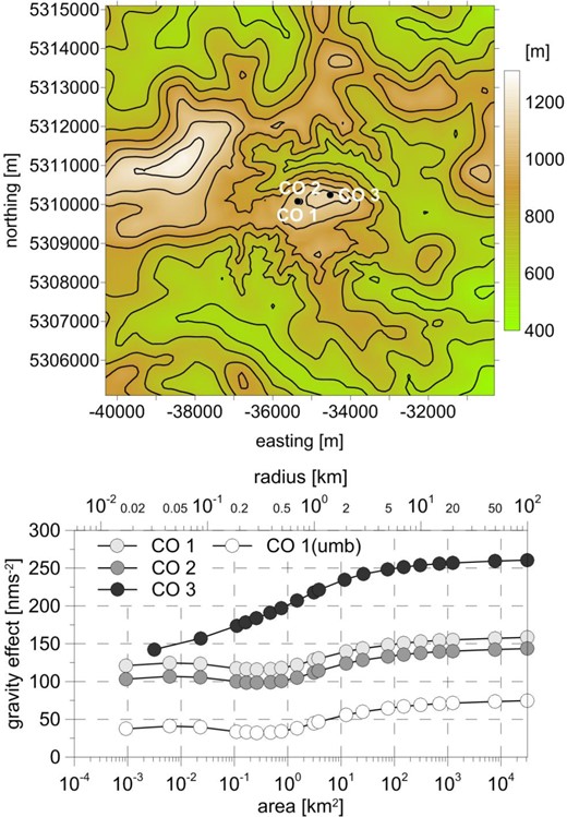
Influence of terrain geometry on local hydrological Newtonian effects.
First, this would be true only if the hydrology model was perfect.
Secondly, while it has been shown, in a few cases, that loading deformations inferred from GRACE may be more consistent with GPS observations than loading deformations calculated from hydrology models (Nahmani et al.2012; Valty et al.2013), this is not the topic of this paper. Here we show that SG measurements are not consistent neither between themselves nor with the gravity time variations estimated either from GRACE or hydrology models. All these discussions do not show that our (and their) calculations are ‘wrong’ and do not change anything on the conclusions of our paper.
Last, but not least, we fully agree with Crossley et al. (2014) ending section 3 by stating that precise hydrology modelling is required to fully explain gravity observations. This can only be achieved by performing comprehensive hydrogeological investigations.
Let us also comment on some details in the comment:
‘In their 1st paragraph on page 4, [MVC] wrote that the Green's function formalism can only be considered for stations above ground’.
In our paper, we wrote: ‘Such assumption is valid for the atmosphere or oceans, but is less adapted for hydrology loading problems, where the load is generally under the sensor’. So, ‘less adapted’ is not ‘can only’.
‘Consequently their conclusion, that is, that hydrology models (or GRACE) cannot be used for precise computation of loading effects, is again false’.
Again we never pretend this in our conclusion. We just wrote: ‘the annual cycles of the SGs are not consistent with predictions computed from GRACE and hydrological models’.
A.4 Common variability and EOF analysis
Crossley et al. (2014) assert that we pretend that correlation and EOF analysis cannot be used if the analysed signals have a common part, which is not written nor even suggested in our paper. Of course, those two techniques only bring information if there is a common part in the analysed signals. By applying an EOF analysis on a set of signals, the time-series associated to the modes indicate the common time variability and the eigenvectors indicate which stations are participating to it, and to which extent. This is very interesting when the properties of the time-series are unknown. When the time-series is an annual, it is better to calculate the amplitude and phase of the seasonal cycle at each station. This provides more information than EOF, as it keeps the phase differences. Again, we do not tell one cannot use the EOF, we simply claim that it will hide the phase differences, which is very useful information. This is a simple consequence of what we demonstrate about correlation in our paper, as EOF analysis is based on the correlation matrix: it is far from optimal when the time-series are dominated by a coherent oscillation.
Applying well-known mathematical tools is no problem, provided that one keeps a critical eye on the results. In particular, the user should not forget that the method is to compute the eigenvectors of the correlation/matrix. This implies that results are not very thrilling if the correlations are weak. One way to test the relevance of the modes is to look at the eigenvalues providing a measure of the per cent variance explained by each mode. When they are low, it means that the mode is not very important for the whole set of time-series. Another relevant information is the eigenvector, which tells how important the modes are for each of the time-series. When the series have a low correlation, a strong component shared by only two time-series might appear as one of the most important modes; then, the other times-series will just contribute as their orthogonal projection on the time-series. This is why not all the modes should be physically interpreted.
‘Crossley et al. (2012) found no large difference in the PC1 solutions whether using the three above-ground stations or the full set of stations, but the second and higher modes clearly reveal the contribution of opposite signals from the below-ground stations, a point missed by [MVC]’.
This statement partially contradicts Abe et al. (2012) who claim that ‘EOF mode 2 contains a strong signal at WE’ (Abe et al.2012, end of p. 9) and WE is a surface station.
‘We should also point out that EOF analysis should not be confined (as in [MVC]) to only the first mode; more than two modes are needed to represent the variability of all the GGP stations as recognized in the previous EOF publications’.
Do Crossley et al. (2014) still believe to be able to interpret the second mode in Abe et al. (2012) paper physically? It is clearly driven by a signal component present at WE, all other SGs have to compensate for by negative eigenvectors.
‘A significant contradiction arises in their EOF treatment, starting after their eq. (3): “…Let us take the seven stations … note that the annual signal was not filtered out” followed two sentences later by “… Here, after filtering for the seasonal cycle we computed the eigenvectors and associated time-series.” Which is correct?’
It seems indeed quite confusing when quoting as Crossley et al. (2014) did. What is actually written reads as:
‘Let us take the seven stations as discussed in Crossley et al. (2012): BH, MB, MC, MO, ST, VI and WE, from 2002.6 to 2007.8; note that the annual signal was not filtered out. For the reasons explained in the beginning of this section, it is difficult to interpret the results if the series contains an annual component: the EOF analysis will extract the seasonal signal as the first mode, even with a non-negligible phase-lag (up to 45°) between the time-series. Actually, the EOF analysis then only allows concluding to the presence of a seasonal signal in all the time-series. Here, after filtering for the seasonal cycle, we computed the eigenvectors and the associated time-series’.
Which is not half as confusing as what Crossley et al. (2014) say in their comment.
‘Despite all of their processing problems, the SG series are overall quite coherent with the numerous GRACE and global hydrology solutions’.
We are glad that Crossley et al. (2014) find coherence in our time-series and seem happy about it, despite our ‘failed’ data processing. Still, we do not see what anyone can learn out of that coherence, if it exists and is significant. We think that we demonstrate it is not, and the comment does not bring any objective argument for the significance of it.
A.5 Local effects on gravity
‘So the averaged total hydrology (mainly the local effect) at all surface locations is indeed the signal seen by GRACE’.
GRACE does not see the averaged local hydrology effects. Instead, GRACE sees the average hydrology effect of an Earth without terrain (see the figure in our appendix)! That is something different. It is what we called |$g_{{\rm L}_{{\rm Smooth}} } (S)$|.
‘Even if the topography is not flat we still have |$g_{\rm L} (S) \approx g_{{\rm L}_{{\rm Smooth}} } (S)$| because surface stations on an uneven terrain approximate |$g_{{\rm L}_{{\rm Smooth}} } (S)$|, especially when combined together over a region L’.
(1) Even in flat topography we have always some kind of umbrella effect (Creutzfeldt et al.2010), the satellite does never see. This effect reduces the amplitude of hydrological signals, depending on the local situation. Therefore, the assumption (1) is questionable even in flat terrain condition. Note, that we did not discuss the umbrella issue in the appendix of our paper for simplicity.
Note that Weise et al. (2012) argue they do not need a correction at BH, because of ‘Considering the large buildings and the sealed and partially drained surrounding of the Bad Homburg station’. If they are right, the SG at BH never represents what GRACE sees.
(2) If terrain is not flat, then the assumption (1) is no longer allowed. Along gentle slopes even surface stations will always experience some kind of compensation of Newtonian effects by hydro masses below and above the sensor. At least the amplitude of hydrological signals is no longer comparable with the downward continued satellite signal. In moderate terrain, the geometry of terrain is an important factor influencing the amplitude of hydrological signals. This is shown by an example from Conrad (CO, moderate terrain, Fig. 1).
The upper panel of Fig. 1 shows the topography. The lower panel shows the Newtonian gravity effect of a soil moisture layer just below the surface (layer thickness 1 m, porosity 30 per cent) as a function of the area covered by the layer. All stations are virtual stations on surface. The Bouguer plate effect is 125.8 nm s−2, but in practice the amplitude of the hydrological signal differs by up to 90 per cent depending on the station location with respect to the terrain geometry. The distance between CO 1 and CO 3 is only 864 m. The close-by stations CO 1 and CO 2, distant by 58 m, differ by 10 per cent. The umbrella effect can reduce the Newtonian effect by more than 50 per cent depending on the size of the umbrella; in this example it amounts 4 × 4 m2 at CO 1 (‘CO 1 (umb)’). At CO 3, a layer of only 500 m radius causes a gravity effect of 200 nm s−2. This is 60 per cent more than the Bouguer plate approximation. Neither the SH nor the Green's function approach will be able to predict local hydrology due to local terrain geometry effects.
Thus we can just not expect any SG site to be representative of other locations surrounding a SG. Therefore, we need hydrology corrections according to what we call remove–restore technique. At this point, all previous studies are lesser consistent than ours.
(3) Only the MC SG station represents a flat topography.
(4) What does mean ‘combined together over a region L’? For the current SG station pattern, there is nothing to combine, as L is the local zone (hectometer scale), and this local zone differs strongly from SG site to SG site, far apart by 200 km or more.
‘Fundamental potential theory says that if stations all lie on a topographic surface the gravity potential can be continued smoothly up to satellite altitudes (apart from atmospheric corrections)’.
This has never been done. Doing this in practice is a challenging type of field transformation, as we have to solve the boundary value problem for uneven and irregular surfaces.
Concerning the comment in the introduction of Crossley et al. (2014):
‘Neumeyer et al. (2006), Weise et al. (2009) and Naujoks et al. (2010), all succeeded in showing that by paying careful attention to the local hydrology contributions, it was possible to reconcile the observations of SG stations with the GRACE data.’
(1) They corrected for the local Newtonian effect, but did not restore |$g_{{\rm L}_{{\rm Smooth}} }$|.
(2) How does this statement fit to the wording ‘We do not need the hydrology everywhere to make the correction, and it is not a futile circular problem’ (last sentence of section 4 of Crossley et al. (2014))? We need local hydrology everywhere at least for correcting for the umbrella effect. And after having corrected for we need to restore that part in an appropriate way.
(3) Crossley et al. (2012) did not apply any correction, while Abe et al. (2012) did, but in an arbitrary, not well argued fashion regarding the extent of the correction zone, and also did not restore |$g_{{\rm L}_{{\rm Smooth}} }$|. Crossley et al. (2014) state also that ‘Corrections for local hydrology are required only if the site hydrology or other factors (e.g. soil, topography) would not be representative of other surface locations surrounding an SG’. Which are the scientific arguments which would allow one to apply a local hydrology correction? Only when it is necessary to support a thesis as done by Abe et al. (2012)? Fig. 1 proves that site hydrology is just not representative of other locations surrounding a SG.
(4) B. Meurers, coauthor of this study, coauthored the paper by Neumeyer et al. (2006). Neumeyer et al. (2006) simply corrected for groundwater effects (where sensors were available) by making use of regression analysis. It was the best they could do at that time, but we would not call it ‘paying careful attention to local hydrological contributions’.
