Abstract

Four different forms of the tensor Green's function for the gravitational gradient tensor, derived in this article, give a theoretical basis for geophysical interpretations of the GOCE-based gravitational gradients in terms of the Earth's mass-density structure. The first form is an invariant expression of the tensor Green's function that can be used to evaluate numerically the gravitational gradients in different coordinate systems (e.g. Cartesian). The second form expresses the gravitational gradients in spherical coordinates (ϑ, φ) with the origin at the north pole as a series of tensor spherical harmonics. This form is convenient to apply when the GOCE data are represented in terms of the gravitational potential as a scalar spherical harmonic series, such as the GOCO03S satellite gravity model. The third form expresses gravitational gradients in spherical coordinates (ψ, α) with the pole at the computation point. The fourth form then expresses the corresponding isotropic kernels in a closed form. The last two forms are used to analyse the sensitivity of the gravitational gradients with respect to lateral distribution of the Earth's mass-density anomalies. They additionally provide a tool for evaluating the omission error of geophysically modelled gravitational gradients and its amplification when the bandwidth-limited GOCE-based gravitational gradients are interpreted at different heights above the Earth's surface. We show that the omission error of the bandwidth-limited mass-density Green's functions for gradiometric data at the GOCE satellite's altitude does not exceed 1 per cent in amplitude when compared to the full-spectrum Green's functions. However, when evaluating the bandwidth-limited Green's functions at lower altitudes, their omission errors are significantly amplified. In this case, we show that the short-wavelength content of the forward-modelled gravitational gradients generated by an a priori density structure of the Earth must be filtered out such that the omission error of the GOCE-based gravitational gradients (i.e. the signal that has not been modelled from the GOCE data) is equal to the omission error of the forward-modelled gravitational gradients. Only after performing such filtering can the GOCE-based gravitational gradients at low altitudes be interpreted in terms of the Earth's density structure. Both the closed and spherical-harmonic forms of the Green's functions allow a direct interpretation in terms of the minimum lateral extent of the Earth that needs to be considered in a regional model constrained by gravitational gradients if the full information provided by the Green's functions is to be retained. We show that this extent (i) is smallest for the vertical–vertical Green's function and (ii) linearly increases with increasing computation-point height. The spectral forms of the gravitational gradients are further used to calculate the sensitivity of the GOCE-based gravitational gradients to the depth of density anomalies, expressed in terms of the harmonic degree of the internal mass-density anomaly. We show that the largest gravitational gradient response is obtained for shallow mass anomalies, and is further amplified as the harmonic degree increases.

1 INTRODUCTION

The gravity field and steady-state ocean circulation explorer (GOCE), launched in 2009, provides gravitational gradients at a perigee height of 255 km with a spatial resolution of 90 km and a precision of 1 mGal (e.g. Rummel et al.2011). The GOCE gravitational gradient data are delivered by its on-board gradiometer. The gradients themselves are not directly measured, but derived from the differences between the accelerations of three pairs of accelerometers (Frommknecht et al.2011). The gravitational gradients are thus determined in the so-called gradiometer reference frame, which co-rotates with the satellite. The gradiometer-reference-frame configuration is such that four gravitational gradients are determined with a high level of accuracy, whereas the other two are less accurate. The GOCE gravitational gradients in the gradiometer reference frame are combined with complementary data from the gravity field missions CHAMP and GRACE (and also with SLR, terrestrial gravity data and satellite altimetry) and the combined global gravity field (GOCO) models are calculated (e.g. Pail et al.2013). In this text, we refer to the GOCE-based gravitational gradients as the gradients calculated from the spherical harmonic expansion of a GOCO model, for example GOCO03S (Mayer-Gürr et al.2012), with full spectral content up to degree and order 220.

The latest GOCO models have improved upon the available information about the terrestrial gravity field in comparison to the EGM2008 model (Pavlis et al.2012) in regions where the quantity and quality of terrestrial gravity data included in the EGM2008 model is poor (Bouman et al.2011; Bouman and Fuchs 2012; Hirt et al.2012). This is particularly evident in less well surveyed parts of the world, for example central Africa, where the noise in the terrestrial gravity data incorporated into the EGM2008 model has been substantially reduced. A number of studies have exploited the capabilities of the new GOCE data in constraining the structure of the Earth's crust and oceans (e.g. Bingham et al.2011; Álvarez et al.2012; Hirt et al.2012; Köther et al.2012; Mariani et al.2013), the lithosphere (Bouman et al.2013) and the upper mantle structure (Fullea et al.2013).

The representation of the gravitational potential of a GOCO model in terms of solid spherical harmonics allows the evaluation of the GOCE-based gravitational gradients at different heights above the Earth's surface, as well as the possibility of interpreting the GOCE-based gravitational gradients in terms of the solid Earth's structure, again at different altitudes. Two different approaches based on the height where the GOCE-based gravitational gradients are interpreted by modelled quantities have been considered. First, for the identification of geological units in unexplored parts of the world, such as the central part of Africa, it is useful to evaluate the GOCE-based gravitational gradients at altitudes close to the Earth's surface, since the gradiometric signal is amplified and better reflects the near-surface geological structure. However, the signal induced by the topographic masses is enhanced at low altitudes and the sensitivity to the uncertainties in topographic-mass density is increased. The standard value of 2670 kg m−3 for topographic-mass density reductions may introduce an undesired error to geophysically modelled gravitational gradients, for instance, in areas of elevated, low-density sediments (e.g. the Congo basin). In addition, the evaluation of the GOCE-based gravitational gradients at low altitudes amplifies not only the signal, but also their omission errors (in general, the omission error is the signal that has not been modelled, Losch et al.2002).

The second approach is based on the fact that a short-wavelength gravitational signal due to near-surface geology is dampened at satellite altitudes more efficiently than a long-wavelength gravitational signal with lithospheric and sublithospheric origins. Hence, studies on lithospheric or upper-mantle structure interpret the GOCE-based gravitational gradients at the satellite's altitudes (Bouman et al.2013; Fullea et al.2013). In the same way, the omission error of forward-modelled gravitational gradients is dampened efficiently at GOCE satellite's altitudes and these gravitational gradients are then easier to compare with the bandwidth-limited GOCE-based gravitational gradients.

The omission error of the GOCE-based gravitational gradients can be mathematically described and its amplification at the computation point located near the Earth's surface numerically estimated. This motivates the work of this paper. We present a detailed and systematic derivation of the mass-density Green's functions for satellite gravitational gradients in both the spherical-harmonic and closed forms. We demonstrate that these two alternative forms provide a mathematical tool for calculating the omission error of the bandwidth-limited gradiometric data at satellite altitude and its amplification when the GOCE-based satellite gravitational gradients are considered at altitudes near the Earth's surface. The spectral forms of the gravitational gradients are further used to calculate the sensitivity of the satellite gravitational gradients to the depth of density anomalies.

There are, in particular, three main questions addressed in this paper. (i) How important is the omission error of the bandwidth-limited Green's functions when the GOCE-based gravitational gradients are interpreted at different heights above the Earth's surface? (ii) How do the gravitational gradients depend on the spatial distribution of the Earth's density structure? (iii) What is the minimum lateral extent of the portion of the Earth that needs to be considered for regional geophysical models constrained by the GOCE-based satellite gravitational gradients if the full information provided by the Green's functions is to be retained?

It is a known fact that the inverse gravimetric problem, that is the determination of the Earth's density structure from knowledge about the external gravitational potential or vertical gravity, is an ill-posed problem since it violates three Hadamard's criteria on the well-posedness of a mathematical model (Hadamard 1923). There is an extensive literature on dealing with ill-posed inverse problems (e.g. Menke 1989; Parker 1994; Xu 1998; Tarantola 2005). In particular, the inverse gravimetric problem has been studied by for example Pěč & Martinec (1984), Sansò et al. (1986), Matyska (1987), Ballani et al. (1993a,b). The ill-posedness of the inverse gradiometric problem, that is the case where the gravitational gradients are interpreted in terms of the Earth's density structure, is of a similar character as that of the inverse gravimetric problem. However, no theoretical study has been published to investigate the differences in these two inverse problems.

It is not the aim of this paper to provide a comprehensive theoretical study of the inverse gradiometric problem, nor to solve it while determining the Earth's density structure over regional scales. For the latter case, we refer to a number of recent efforts to interpret the GOCE-based gravitational gradients in terms of a regional density model (Braitenberg et al.2011; Álvarez et al.2012; Bouman et al.2013; Fullea et al.2013; Martinec & Fullea 2013). In fact, the difficulties when carrying out these interpretations have motivated the theoretical work presented hereafter.

2 GREEN'S FUNCTIONS FOR THE GRAVITATIONAL POTENTIAL, VECTOR AND GRADIENT TENSOR

The gravitational potential V generated by the volume density distribution ϱ inside the Earth with a volume |${\cal V}$| is expressed by the Newton integral (e.g. Kellogg 1954; Heiskanen & Moritz 1967) as,
\begin{equation} V(\vec{r})=\kappa \int \limits _{\cal V}^{}\varrho (\vec{r}^{\prime }) \,G(\vec{r},\vec{r}^{\prime })\, {\rm d}V, \end{equation}
(1)
where κ is Newton's gravitational constant and |$G(\vec{r},\vec{r}^{\prime })$| is the reciprocal distance between the computation point |$\vec{r}$| and an integration point |$\vec{r}^{\prime }$| of the mass element |$dm=\varrho (\vec{r}^{\prime })dV$|⁠,
\begin{equation} G(\vec{r},\vec{r}^{\prime })={1\over L(\vec{r},\vec{r}^{\prime })}. \end{equation}
(2)
The function |$G(\vec{r},\vec{r}^{\prime })$| satisfies Poisson's equation for the gravitational potential V with the right-hand side equal to the Dirac delta function |$\delta (\vec{r}-\vec{r}^{\prime })$|⁠. In the terminology of partial differential equations, |$G(\vec{r},\vec{r}^{\prime })$| is the Green's function for gravitational potential (e.g. Renardy & Rogers 1993).
Applying successively the operator ‘grad’ to the potential V results in the gravitational vector |$\vec{g}={\rm grad}\,V$| and the gravitational gradient (or gradiometric) tensor |${\Gamma }={\rm grad\ grad}\,V$|⁠,
\begin{equation} \vec{g}(\vec{r})=\kappa \int \limits _{\cal V}^{}\varrho (\vec{r}^{\prime })\, \vec{G}(\vec{r},\vec{r}^{\prime })\, {\rm d}V, \end{equation}
(3)
\begin{equation} {\Gamma }(\vec{r})=\kappa \int \limits _{\cal V}^{}\varrho (\vec{r}^{\prime })\, {\bf G}(\vec{r},\vec{r}^{\prime })\, {\rm d}V. \end{equation}
(4)
The respective vector and tensor Green's functions for gravitation and gravitational gradient are
\begin{equation} \vec{G}(\vec{r},\vec{r}^{\prime })={\rm grad}{1\over L}, \end{equation}
(5)
\begin{equation} {\bf G}(\vec{r},\vec{r}^{\prime })={\rm grad\ grad}{1\over L}. \end{equation}
(6)
Expressing the distance L in Cartesian coordinates and applying successively the operator ‘grad’ to 1/L results in
\begin{equation} \vec{G}(\vec{r},\vec{r}^{\prime })= -{\vec{r}-\vec{r}^{\prime }\over L^3}, \end{equation}
(7)
\begin{equation} {\bf G}(\vec{r},\vec{r}^{\prime })= -{1\over L^3}\Big [{\bf I}-{3(\vec{r}-\vec{r}^{\prime })\otimes (\vec{r}-\vec{r}^{\prime }) \over L^2}\Big ], \end{equation}
(8)
where |${\bf I}$| is the second-order identity tensor and the symbol ⊗ stands for the dyadic product of vectors.

3 GREEN'S FUNCTIONS IN SPHERICAL-HARMONIC FORM

3.1 Gravitational potential

To represent the Green's function |$G(\vec{r},\vec{r}^{\prime })$| in terms of spherical harmonics, we express the distance L between the points |$\vec{r}$| and |$\vec{r}^{\prime }$| by the cosine theorem,
\begin{equation} L(r,\psi ,r^{\prime })=\sqrt{r^2+r^{\prime 2}-2rr^{\prime }\cos \psi }, \end{equation}
(9)
where r and r are the magnitudes of vectors |$\vec{r}$| and |$\vec{r}^{\prime }$|⁠, respectively, and ψ is the angular distance between the geocentric directions of |$\vec{r}$| and |$\vec{r}^{\prime }$|⁠. For r > r, the reciprocal distance 1/L can be expanded into a uniformly convergent series of Legendre polynomials Pj(cos ψ) (e.g. Arfken 1968),
\begin{equation} {1\over L(r,\psi ,r^{\prime })} ={1\over r}\sum _{j=0}^\infty \bigg ({r^{\prime }\over r}\bigg )^{j}P_j(\cos \psi ). \end{equation}
(10)
The Laplace addition theorem for scalar spherical harmonics reads as (Varshalovich et al.1989)
\begin{equation} P_j(\cos \psi )={4\pi \over 2j+1}\sum _{m=-j}^j Y^*_{jm}(\Omega ^{\prime })Y_{jm}(\Omega ), \end{equation}
(11)
where Ω represents the co-latitude ϑ and longitude φ of the computation point, Ω ≡ (ϑ, φ), and Ω refers to the co-latitude ϑ and longitude φ of a mass integration point, Ω ≡ (ϑ, φ), Yjm(Ω) are the fully normalized scalar spherical harmonics of spherical degree and azimuthal order j and m, and the asterisk denotes the complex conjugate. Substituting eq. (11) into eq. (10) results in
\begin{equation} {1\over L(r,\psi ,r^{\prime })} ={1\over r}\sum _{j=0}^\infty {4\pi \over 2j+1}\bigg ({r^{\prime }\over r}\bigg )^{j} \sum _{m=-j}^j Y^*_{jm}(\Omega ^{\prime })Y_{jm}(\Omega ). \end{equation}
(12)
In view of eqs (1) and (2), this is the spherical-harmonic representation of the mass-density Green's function G for the gravitational potential V in the case where the radial distance of the computation point from the geocentre is greater than the radial distance of a mass integration point from the geocentre (r > r).

3.2 Gravitational vector

To represent the vector Green's function |$\vec{G}(\vec{r},\vec{r}^{\prime })$| for the gravitational vector |$\vec{g}$|⁠, we use the following gradient formula (Varshalovich et al.1989)
\begin{eqnarray} {\rm grad\, \displaystyle }\big [f(r)Y_{jm}(\Omega )\big ]= {df(r)\over dr} {\bf Y}_{jm}^{(-1)}(\Omega ) +\sqrt{j(j+1)}\,{f(r)\over r} {\bf Y}_{jm}^{(1)}(\Omega ),\nonumber \\ \end{eqnarray}
(13)
where |${\bf Y}_{jm}^{(\lambda )}(\Omega )$| are spheroidal vector spherical harmonics. The gradient of 1/L with respect to the coordinates of the computation point is then expressed as
\begin{eqnarray} {\rm grad\, \displaystyle }{1\over L} &=&{1\over r^2}\sum _{j=0}^\infty {4\pi \over 2j+1}\bigg ({r^{\prime }\over r}\bigg )^{j} \sum _{m=-j}^j Y^*_{jm}(\Omega ^{\prime })\nonumber \\ &&\times \, \Big [-(j+1){\bf Y}_{jm}^{(-1)}(\Omega ) +\sqrt{j(j+1)}{\bf Y}_{jm}^{(1)}(\Omega )\Big ]. \end{eqnarray}
(14)
The representation of |${\bf Y}_{jm}^{(\pm 1)}(\Omega )$| in the spherical unit base vectors |$\vec{e}_r$|⁠, |$\vec{e}_\vartheta$| and |$\vec{e}_\varphi$| is then written as (Varshalovich et al.1989)
\begin{eqnarray} {\bf Y}_{jm}^{(-1)}(\Omega )&=&\vec{e}_r Y_{jm}(\Omega ),\nonumber \\ {\bf Y}_{jm}^{(+1)}(\Omega )&=&{1\over \sqrt{j(j+1)}}\bigg ( {\partial Y_{jm}(\Omega )\over \partial \vartheta }\,\vec{e}_\vartheta +{1\over \sin \vartheta }{\partial Y_{jm}(\Omega )\over \partial \varphi }\,\vec{e}_\varphi \bigg ). \end{eqnarray}
(15)
Substituting eq. (15) into eq. (14) and denoting
\begin{equation} t:={r^{\prime }\over r} \end{equation}
(16)
yields
\begin{eqnarray} {\rm grad\, \displaystyle }{1\over L} &=&{1\over r^2}\sum _{j=0}^\infty {4\pi \over 2j+1}t^j \sum _{m=-j}^j Y^*_{jm}(\Omega ^{\prime }) \bigg [-(j+1)Y_{jm}(\Omega )\vec{e}_r \nonumber \\ &&+\; {\partial Y_{jm}(\Omega )\over \partial \vartheta }\,\vec{e}_\vartheta +{1\over \sin \vartheta }{\partial Y_{jm}(\Omega )\over \partial \varphi }\,\vec{e}_\varphi \bigg ]. \end{eqnarray}
(17)
In view of eqs (3) and (5), this is the spherical-harmonic representation of the mass-density Green's function |$\vec{G}$| for the gravitation vector |$\vec{g}$| in the case where the radial distance of the computation point from the geocentre is greater than the radial distance of a mass integration point from the geocentre (r > r).
As for the mass-density Green's function for the potential, using the angular distance ψ makes explicit the sensitivity of the Green's function to the angular distance between the computation point and a mass source. In addition to general spherical coordinates (ϑ, φ), we consider spherical coordinates (ψ, α) with the origin located at the computation point, where the azimuth α is reckoned from the north. Recalling the addition theorems for the first-order derivatives of scalar spherical harmonics (Grafarend 2001; Martinec 2003),
\begin{eqnarray} &&\!\!\!\!&&{\displaystyle \sum _{m=-j}^j\displaystyle {\displaystyle \partial Y_{jm}(\Omega ) \over \displaystyle \partial \vartheta }Y_{jm}^*(\Omega ^{\prime })=\displaystyle {\displaystyle 2j+1\over \displaystyle 4\pi }\cos \alpha \sin \psi \, \displaystyle {\displaystyle dP_j(\cos \psi )\over \displaystyle d\cos \psi },}\nonumber \\ &&\!\!\!\!\displaystyle \sum _{m=-j}^j \displaystyle {\displaystyle 1\over \displaystyle \sin \vartheta } \displaystyle {\displaystyle \partial Y_{jm}(\Omega ) \over \displaystyle \partial \varphi }Y_{jm}^*(\Omega ^{\prime }) =-\displaystyle {\displaystyle 2j+1\over \displaystyle 4\pi }\sin \alpha \sin \psi \, \displaystyle {\displaystyle dP_j(\cos \psi )\over \displaystyle d\cos \psi },\nonumber \\ \end{eqnarray}
(18)
and the addition theorem for scalar spherical harmonics, eq. (11), the mass-density Green's function for gravitation, |$\vec{G}={\rm grad\, \displaystyle }{(1/L)}$|⁠, is expressed in terms of the isotropic parts that are dependent upon the angular distance ψ between the computational point and an integration point, and their positions in the radial direction, and the parts depending on the azimuth α,
\begin{equation} {\rm grad\, \displaystyle }{1\over L}={1\over r^2} [ K_r(t,x)\vec{e}_r +K_\Omega (t,x)(\cos \alpha \,\vec{e}_\vartheta -\sin \alpha \,\vec{e}_\varphi ) ], \end{equation}
(19)
where x = cos ψ has been substituted for abbreviation. The two isotropic kernels Kr(t, x) and |$K_\Omega (t,x)$| are given by an infinite series of Legendre polynomials and their first derivatives,
\begin{eqnarray} K_r(t,x)&=&-\sum _{j=0}^\infty (j+1) t^jP_j(x),\nonumber \\ K_\Omega (t,x)&=&\sqrt{1-x^2}\sum _{j=0}^\infty t^j {dP_j(x)\over dx}. \end{eqnarray}
(20)

3.3 Gravitational gradient tensor

Applying the operator ‘grad’ twice to 1/L and using eq. (12), we obtain
\begin{eqnarray} {\rm grad\, \displaystyle }{\rm grad\, \displaystyle }{1\over L} &=&\sum _{j=0}^\infty {4\pi \over 2j+1}(r^{\prime })^j\nonumber \\ &&\times\, \sum _{m=-j}^j Y^*_{jm}(\Omega ^{\prime }) \,{\rm grad\, \displaystyle }{\rm grad\, \displaystyle }[r^{-j-1} Y_{jm}(\Omega )]. \end{eqnarray}
(21)
Meanwhile, Martinec (2003) showed that
\begin{eqnarray} &&\!\!\!\!&&{{\rm grad\, \displaystyle }{\rm grad\, \displaystyle }[r^{-j-1} Y_{jm}(\Omega )]=r^{-j-3}\bigg [ (j+1)(j+2){\bf Z}_{jm}^{(1)}(\Omega )}\nonumber \\ &&\!\! -\,2(j+2){\bf Z}_{jm}^{(2)}(\Omega ) +{1\over 2}{\bf Z}_{jm}^{(3)}(\Omega ) +{j+2\over 2j}{\bf Z}_{jm}^{(4)}(\Omega ) \bigg ], \end{eqnarray}
(22)
where |${\bf Z}_{jm}^{(\lambda )}(\Omega )$| are spheroidal tensor spherical harmonics. Creating the dyadic products of spherical unit base vectors |$\vec{e}_r$|⁠, |$\vec{e}_\vartheta$| and |$\vec{e}_\varphi$| and taking the symmetric part of the result, we define the symmetric spherical dyadics
\begin{equation} {\bf e}_{ij}=[\vec{e}_i\otimes \vec{e}_j]_{\rm sym}, \quad \quad i,j\in \lbrace r,\vartheta ,\varphi \rbrace . \end{equation}
(23)
The dyadic components of the tensor spherical harmonics are then given by (Martinec 2000)
\begin{eqnarray} {\bf Z}_{jm}^{(1)}(\Omega )&=&Y_{jm}(\Omega ){\bf e}_{rr},\nonumber \\ {\bf Z}_{jm}^{(2)}(\Omega )&=&E_{jm}(\Omega ){\bf e}_{r\vartheta } +F_{jm}(\Omega ){\bf e}_{r\varphi }, \nonumber \\ {\bf Z}_{jm}^{(3)}(\Omega )&=& G_{jm}(\Omega )\left({\bf e}_{\vartheta \vartheta }-{\bf e}_{\varphi \varphi }\right) +2\,H_{jm}(\Omega ){\bf e}_{\vartheta \varphi },\nonumber \\ {\bf Z}_{jm}^{(4)}(\Omega )&=&-j(j+1)Y_{jm}(\Omega ) \left({\bf e}_{\vartheta \vartheta }+{\bf e}_{\varphi \varphi }\right), \end{eqnarray}
(24)
where the abbreviations have the following meanings,
\begin{eqnarray} E_{jm}(\Omega )&=&{\partial Y_{jm}(\Omega )\over \partial \vartheta },\nonumber \\ F_{jm}(\Omega )&=& {1\over \sin \vartheta }{\partial Y_{jm}(\Omega )\over \partial \varphi }, \nonumber \\ G_{jm}(\Omega )&=& \left({\partial ^2 \over \partial \vartheta ^2} -\cot \vartheta {\partial \over \partial \vartheta } -{1\over \sin ^2\vartheta }{\partial ^2\over \partial \varphi ^2} \right)Y_{jm}(\Omega ),\nonumber \\ H_{jm}(\Omega )&=&{\partial \over \partial \vartheta }\left( {1\over \sin \vartheta }{\partial Y_{jm}(\Omega )\over \partial \varphi }\right). \end{eqnarray}
(25)
Substituting eq. (22) into eq. (21) and using eqs (23)–(25) yields
\begin{eqnarray} {\rm grad\, \displaystyle }{\rm grad\, \displaystyle }{1\over L} &=&{1\over r^3}\sum _{j=0}^\infty {4\pi \over 2j+1}t^j \sum _{m=-j}^j Y^*_{jm}(\Omega ^{\prime })\nonumber \\ &&\times\, \bigg [(j+1)(j+2)Y_{jm}(\Omega ){\bf e}_{rr}\nonumber \\ && -\,2(j+2)\left(E_{jm}(\Omega ){\bf e}_{r\vartheta } +F_{jm}(\Omega ){\bf e}_{r\varphi }\right)\nonumber \\ && +\,{1\over 2}G_{jm}(\Omega )\left({\bf e}_{\vartheta \vartheta }-{\bf e}_{\varphi \varphi }\right) +H_{jm}(\Omega ){\bf e}_{\vartheta \varphi }\nonumber \\ && -\,{1\over 2}(j+1)(j+2)Y_{jm}(\Omega ) \left({\bf e}_{\vartheta \vartheta }+{\bf e}_{\varphi \varphi }\right)\bigg ]. \end{eqnarray}
(26)
In view of eqs (4) and (6), this is the spherical-harmonic representation of the mass-density Green's function |${\bf G}$| for the gravitational gradient tensor |${\bf {\Gamma }}$| in the case where the radial distance of the computation point from the geocentre is greater than the radial distance of a mass integration point from the geocentre (r > r).
As for the mass-density Green's functions for the potential and gravitational vector, we express the Green's function for the gravitational gradient tensor in terms of the spherical coordinates (ψ, α). Recalling the addition theorems for the 2nd order derivatives of scalar spherical harmonics (Martinec 2003),
\begin{eqnarray} &&\!\!\!\!&&{\displaystyle \sum _{m=-j}^j E_{jm}(\Omega )Y_{jm}^*(\Omega ^{\prime })=\displaystyle {\displaystyle 2j+1\over \displaystyle 4\pi }\cos \alpha \sin \psi \displaystyle {\displaystyle dP_j(\cos \psi )\over \displaystyle d\cos \psi },}\nonumber\\ &&\!\!\!\!\displaystyle \sum _{m=-j}^j F_{jm}(\Omega )Y_{jm}^*(\Omega ^{\prime })=-\displaystyle {\displaystyle 2j+1\over \displaystyle 4\pi }\sin \alpha \sin \psi \displaystyle {\displaystyle dP_j(\cos \psi )\over \displaystyle d\cos \psi },\nonumber \\ &&\!\!\!\!\displaystyle \sum _{m=-j}^j G_{jm}(\Omega )Y_{jm}^*(\Omega ^{\prime })=\displaystyle {\displaystyle 2j+1\over \displaystyle 4\pi }\cos 2\alpha \sin ^2\psi \displaystyle {\displaystyle d^2P_j(\cos \psi )\over \displaystyle d(\cos \psi )^2},\nonumber\\ &&\!\!\!\!\displaystyle \sum _{m=-j}^j H_{jm}(\Omega )Y_{jm}^*(\Omega ^{\prime })=-\displaystyle {\displaystyle 2j+1\over \displaystyle 4\pi }\sin 2\alpha \sin ^2\psi \displaystyle {\displaystyle d^2P_j(\cos \psi )\over \displaystyle d(\cos \psi )^2}, \end{eqnarray}
(27)
and the addition theorem for scalar spherical harmonics, eq.(11), the Green's function for the gravitational gradient tensor, |${\bf G}={\rm grad\, \displaystyle }{\rm grad\, \displaystyle }(1/L)$|⁠, is expressed in terms of the isotropic components that depend upon the angular distance ψ and those components that are dependent upon the azimuth α,
\begin{eqnarray} {\rm grad\, \displaystyle }{\rm grad\, \displaystyle }{1\over L}\!&=&\!{1\over r^3}\bigg [K_{rr}(t,x){\bf e}_{rr} +2K_{r\Omega }(t,x)(\cos \alpha \,{\bf e}_{r\vartheta }-\sin \alpha \,{\bf e}_{r\varphi }) \nonumber \\ &&+\,K_{\Omega \Omega }(t,x)(\cos 2\alpha \, ({\bf e}_{\vartheta \vartheta }-{\bf e}_{\varphi \varphi }) -2\sin 2\alpha \,{\bf e}_{\vartheta \varphi } )\nonumber \\ && -\,{1\over 2}K_{rr}(t,x)({\bf e}_{\vartheta \vartheta }+{\bf e}_{\varphi \varphi }) \bigg ]. \end{eqnarray}
(28)
Note that, as expected, the trace of |${\bf G}$| for |$\vec{r}\ne \vec{r}^{\prime }$| vanishes since the function |$1/L(\vec{r},\vec{r}^{\prime })$| satisfies Poisson's equation with the right-hand side equal to the Dirac delta function |$\delta (\vec{r}-\vec{r}^{\prime })$|⁠,
\begin{equation} {\rm Tr}\ {\bf G}=0. \end{equation}
(29)
The three isotropic kernels Krr(t, x), KrΩ(t, x) and KΩΩ(t, x) are given by an infinite series of Legendre polynomials and their first and second derivatives,
\begin{eqnarray} K_{rr}(t,x)&=&\sum _{j=0}^\infty (j+1)(j+2) t^jP_j(x),\nonumber \\ K_{r\Omega }(t,x)&=&-\sqrt{1-x^2}\sum _{j=0}^\infty (j+2) t^j {dP_j(x)\over dx},\nonumber \\ K_{\Omega \Omega }(t,x)&=&{1\over 2}(1-x^2)\sum _{j=0}^\infty t^j {d^2P_j(x)\over dx^2}. \end{eqnarray}
(30)
The Legendre polynomials and their derivatives can alternatively be expressed in terms of the fully normalized associated Legendre polynomials Pjm(x) of the azimuthal order m = 0, 1 and 2, respectively, as (Varshalovich et al.1989)
\begin{eqnarray} K_{rr}(t,x)&=&\sum _{j=0}^\infty (j+1)(j+2)\sqrt{4\pi \over 2j+1}\, t^jP_{j0}(x),\nonumber \\ K_{r\Omega }(t,x)&=&\sum _{j=0}^\infty (j+2)\sqrt{j(j+1)}\sqrt{4\pi \over 2j+1}\, t^jP_{j1}(x),\nonumber \\ K_{\Omega \Omega }(t,x)&=&{1\over 2}\sum _{j=0}^\infty \sqrt{(j-1)j(j+1)(j+2)} \sqrt{4\pi \over 2j+1}\,t^j P_{j2}(x).\nonumber \\ \end{eqnarray}
(31)

4 CLOSED FORM OF THE ISOTROPIC KERNELS OF THE GRAVITATIONAL VECTOR AND GRADIENT TENSOR

4.1 Gravitational vector

Complementary to the infinite series for the isotropic kernels Kr(t, x) and |$K_\Omega (t,x)$|⁠, [see eq. (20)], we now express these kernels in closed forms. We first apply the gradient operator to 1/L, which in spherical coordinates (ϑ, φ) is written as
\begin{equation} {\rm grad\, \displaystyle }{1\over L}\!=\!{\partial \over \partial r}\bigg ({1\over L}\bigg )\vec{e}_r \!+\!{1\over r}{\partial \over \partial \vartheta }\bigg ({1\over L}\bigg )\vec{e}_\vartheta \!+\!{1\over r\sin \vartheta }{\partial \over \partial \varphi }\bigg ({1\over L}\bigg )\vec{e}_\varphi . \end{equation}
(32)
The partial derivative of 1/L with respect to r is obtained by differentiating eq. (9) with respect to r,
\begin{equation} {\partial \over \partial r}\bigg ({1\over L}\bigg )=-{r-r^{\prime }x\over L^3}=-{1-tx\over r^2g^3}, \end{equation}
(33)
where |$g\equiv g(t,x)=\sqrt{1+t^2-2tx}$|⁠, −1 ≤ x ≤ 1, 0 < t ≤ 1, is the reciprocal generating function of the Legendre polynomials (e.g. Arfken 1968). The partial derivatives of 1/L with respect to ϑ and φ, respectively, can be expressed in terms of the derivative of 1/L with respect to cos ψ. By the chain rule of differentiation, Martinec (2003) showed that
\begin{eqnarray} {\partial \over \partial \vartheta }&=&\cos \alpha \,\sin \psi {\partial \over \partial \cos \psi }, \nonumber \\ {1\over \sin \vartheta }{\partial \over \partial \varphi }&=& -\sin \alpha \,\sin \psi {\partial \over \partial \cos \psi }. \end{eqnarray}
(34)
Hence,
\begin{eqnarray} {\partial \over \partial \vartheta }\bigg ({1\over L}\bigg ) &=&\cos \alpha \,\sin \psi {\partial \over \partial \cos \psi }\bigg ({1\over L}\bigg )\nonumber \\ &=&\cos \alpha \,\sin \psi \,{rr^{\prime }\over L^3}=\cos \alpha \,\sin \psi \,{t\over r^2g^3}. \end{eqnarray}
(35)
Likewise,
\begin{equation} {1\over \sin \vartheta }{\partial \over \partial \varphi }\bigg ({1\over L}\bigg ) =-\sin \alpha \,\sin \psi \,{t\over r^2g^3}. \end{equation}
(36)
Substituting eqs (33), (35) and (36) to eq. (32) thus gives
\begin{eqnarray} {\rm grad\, \displaystyle }{1\over L}={1\over r^2g^3} [-(1-tx)\vec{e}_r +t\sin \psi (\cos \alpha \,\vec{e}_\vartheta -\sin \alpha \,\vec{e}_\varphi )]. \end{eqnarray}
(37)
Comparing this with eq. (19) in turn yields
\begin{eqnarray} K_r(t,x)&:=&-{1-tx\over g^3}, \nonumber \\ K_\Omega (t,x)&:=&\sqrt{1-x^2}\,{t\over g^3}. \end{eqnarray}
(38)
These are the closed forms of the isotropic kernels of the mass-density Green's function for gravitation.

4.2 Gravitational gradient tensor

We continue deriving the closed form of the mass-density Green's function for the gravitational gradient tensor. Eq. (28) implies that to express the kernels Krr(t, x), KrΩ(t, x) and KΩΩ in a closed form, it is sufficient to find the closed form of the rr, rϑ and ϑφ components of the |${\rm grad\, \displaystyle }{\rm grad\, \displaystyle }(1/L)$| tensor.

By differentiating eq. (33) with respect to r, the rr component of |${\rm grad\, \displaystyle }{\rm grad\, \displaystyle }(1/L)$| is given by
\begin{eqnarray} \Big [{\rm grad\, \displaystyle }{\rm grad\, \displaystyle }{1\over L}\Big ]_{rr}&=&{\partial ^2\over \partial r^2}\bigg ({1\over L}\bigg ) =-{1\over L^3}+{3\over L^5}(r-r^{\prime }x)^2 \nonumber \\ &=&{1\over r^3}\Big (-{1\over g^3}+{3(1-tx)^2\over g^5}\Big ), \end{eqnarray}
(39)
where g is defined from eq. (33). The rϑ component of |${\rm grad\, \displaystyle }{\rm grad\, \displaystyle }(1/L)$| follows on as:
\begin{equation} \Big [{\rm grad\, \displaystyle }{\rm grad\, \displaystyle }{1\over L}\Big ]_{r\vartheta } ={1\over r}{\partial ^2\over \partial r\vartheta }\bigg ({1\over L}\bigg ) -{1\over r^2}{\partial \over \partial \vartheta }\bigg ({1\over L}\bigg ). \end{equation}
(40)
The differentiation of eq. (35) with respect to r gives
\begin{eqnarray} {\partial ^2\over \partial r\partial \vartheta }\bigg ({1\over L}\bigg ) &=&\cos \alpha \,\sin \psi \,{r^{\prime }\over L^3}\Big (1-{3r(r-r^{\prime }x)\over L^2}\Big ) \nonumber \\ &=&{1\over r}{\partial \over \partial \vartheta }\bigg ({1\over L}\bigg ) -\cos \alpha \,\sin \psi {3rr^{\prime }(r-r^{\prime }x)\over L^5}. \end{eqnarray}
(41)
Hence,
\begin{eqnarray} \Big [{\rm grad\, \displaystyle }{\rm grad\, \displaystyle }{1\over L}\Big ]_{r\vartheta } &=&-\cos \alpha \,\sin \psi \, {3r^{\prime }(r-r^{\prime }x)\over L^5} \nonumber \\ &=&-\cos \alpha \,\sin \psi \, {3t(1-tx)\over r^3g^5}. \end{eqnarray}
(42)
The ϑφ component of |${\rm grad\, \displaystyle }{\rm grad\, \displaystyle }(1/L)$| in turn is given as
\begin{eqnarray} \Big [{\rm grad\, \displaystyle }{\rm grad\, \displaystyle }{1\over L}\Big ]_{\vartheta \varphi } &=&{1\over r^2\sin \vartheta }{\partial ^2\over \partial \vartheta \partial \varphi } \bigg ({1\over L}\bigg ) -{\cos \vartheta \over r^2\sin ^2\vartheta }{\partial \over \partial \varphi }\bigg ({1\over L}\bigg ) \nonumber \\ &=& {1\over r^2}{\partial \over \partial \vartheta }\bigg [{1\over \sin \vartheta } {\partial \over \partial \varphi } \bigg ({1\over L}\bigg )\bigg ]. \end{eqnarray}
(43)
Martinec (2003) showed that
\begin{equation} {\partial \over \partial \vartheta }\bigg ({1\over \sin \vartheta } {\partial \over \partial \varphi }\bigg )= -{1\over 2}\sin 2\alpha \sin ^2\psi {\partial ^2\over \partial (\cos \psi )^2}. \end{equation}
(44)
Making use of this differential identity in eq. (43) and performing the second-order derivatives of 1/L with respect to cos ψ, that is
\begin{equation} {\partial ^2\over \partial (\cos \psi )^2}\bigg ({1\over L}\bigg )={3r^2(r^{\prime })^2\over L^5} ={3t^2\over rg^5}, \end{equation}
(45)
results in
\begin{equation} \Big [{\rm grad\, \displaystyle }{\rm grad\, \displaystyle }{1\over L}\Big ]_{\vartheta \varphi } =-{1\over 2}\sin 2\alpha \sin ^2\psi {3t^2\over r^3g^5}. \end{equation}
(46)
Finally, the comparison of eq. (28) with eqs (39), (42) and (46), respectively, gives
\begin{eqnarray} K_{rr}(t,x)&=&-{1\over g^3}+{3(1-tx)^2\over g^5},\nonumber \\ K_{r\Omega }(t,x)&=&-\sqrt{1-x^2}\,{3t(1-tx)\over g^5},\nonumber \\ K_{\Omega \Omega }(t,x)&=&{1\over 2}(1-x^2){3t^2\over g^5}. \end{eqnarray}
(47)
These are the closed forms of the isotropic kernels of the mass-density Green's function for the gravitational gradient tensor.

5 DECOMPOSITION OF THE GRAVITATIONAL GRADIENT TENSOR

Eq. (28) in combination with eq. (4) shows that the five independent components of the gravitational gradient tensor |${\bf {\Gamma }}$| can be grouped into three second-order tensors as follows:
\begin{equation} {\bf {\Gamma }}={\bf {\Gamma }}_{rr}+{\bf {\Gamma }}_{r\Omega }+{\bf {\Gamma }}_{\Omega \Omega }. \end{equation}
(48)
The tensors |${\bf {\Gamma }}_{rr}$|⁠, |${\bf {\Gamma }}_{r\Omega }$| and |${\bf {\Gamma }}_{\Omega \Omega }$| can be referred to as the vertical-vertical, vertical-horizontal and horizontal-horizontal gravitational gradients (Martinec 2003; Bölling & Grafarend 2005), respectively, since their componental forms are
\begin{eqnarray} {\bf {\Gamma }}_{rr}&=&D_{rr} \Big [{\bf e}_{rr}-{1\over 2}({\bf e}_{\vartheta \vartheta }+{\bf e}_{\varphi \varphi })\Big ], \nonumber \\ {\bf {\Gamma }}_{r\Omega }&=&2D_{r\vartheta }\,{\bf e}_{r\vartheta }-2D_{r\varphi }\,{\bf e}_{r\varphi },\nonumber \\ {\bf {\Gamma }}_{\Omega \Omega }&=&D_{\vartheta \vartheta \varphi \varphi } \big ({\bf e}_{\vartheta \vartheta }-{\bf e}_{\varphi \varphi }\big ) -2D_{\vartheta \varphi }\,{\bf e}_{\vartheta \varphi }. \end{eqnarray}
(49)
In spherical coordinates (ψ, α), the components of the tensors |${\bf {\Gamma }}_{rr}$|⁠, |${\bf {\Gamma }}_{r\Omega }$| and |${\bf {\Gamma }}_{\Omega \Omega }$| evaluated at the computation point are expressed by five radially dependent functions,
\begin{eqnarray} D_{rr}(r)&=&{\kappa \over r^3} \int \limits _{\cal V}^{}\varrho (\vec{r}^{\prime })\,K_{rr}(t,\cos \psi )\,dV, \nonumber \\ \left\lbrace \begin{array}{c}D_{r\vartheta }(r)\\ D_{r\varphi }(r) \end{array} \right\rbrace &=&{\kappa \over r^3} \int \limits _{\cal V}^{}\varrho (\vec{r}^{\prime })\,K_{r\Omega }(t,\cos \psi ) \left\lbrace \begin{array}{l}\cos \alpha \\ \sin \alpha \end{array} \right\rbrace \,dV,\nonumber \\ \left\lbrace \begin{array}{c}D_{\vartheta \vartheta \varphi \varphi }(r)\\ D_{\vartheta \varphi }(r) \end{array} \right\rbrace &=&{\kappa \over r^3} \int \limits _{\cal V}^{}\varrho (\vec{r}^{\prime })\,K_{\Omega \Omega }(t,\cos \psi ) \left\lbrace \begin{array}{l}\cos 2\alpha \\ \sin 2\alpha \end{array} \right\rbrace \,dV. \end{eqnarray}
(50)
Given a computation point, the gravitational gradient tensor |${\bf {\Gamma }}$| depends on the height of this point above the Earth's surface and on the Earth's density distribution with respect to the computation point. The former is expressed by the dependency of the isotropic kernels Krr, KrΩ and KΩΩ on the radius of the computation point r (t = r/r). The later is expressed by the mass density function |$\varrho (\vec{r}^{\prime })$| and the dependency of Krr, KrΩ and KΩΩ on (i) the depth of the mass element |$dm=\varrho (\vec{r}^{\prime })dV$|⁠, via the radius r in parameter t, (ii) the spherical distance ψ between the mass element dm and the computation point, and (iii) the azimuthal direction α of mass element dm with respect to the computation point. In the following two sections, we explore the dependency of the Green's functions on r, ψ and r, respectively.

6 APPLICATIONS

6.1 Omission error and spatial dependency of the gravitational gradient tensor

Let us first investigate the sensitivity of the gravitational gradients to the height above the Earth's surface where they are computed. The left-hand panel of Fig. 1 shows the isotropic kernels Krr(t, cos ψ) (red solid line), KrΩ(t, cos ψ) (green solid line) and KΩΩ(t, cos ψ) (blue solid line) evaluated by the closed forms (47) for angular distances 0° ≤ ψ ≤ 6° and t = 0.96224, which corresponds to the GOCE perigee height of 255 km. The graphs of the kernels are bell-shaped (terminology used by Eshagh 2011) but with different positions of their maximum values. Function Krr has its maximum at point ψ = 0° and decreases monotonically to zero with increasing angular distance ψ, whereas functions KrΩ and KΩΩ vanish at ψ = 0°, increase their amplitudes for increasing distance ψ, before reaching their maximum amplitudes at ψmax ≈ 1.1° and ψmax ≈ 1.8°, respectively, and then monotonically decreasing with distance ψ. Quantitatively, the amplitude of function Krr decreases to <1 per cent of its maximum value for distances ψ > 3°, while functions KrΩ and KΩΩ still have significant non-zero amplitudes from that distance, while their amplitudes are less than 10−2 × KrΩ(t, ψmax) and 10−2 × KΩΩ(t, ψmax) at distances ψ > 10° and ψ > 18°, respectively.

Figure 1.

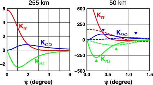
Left-hand panel: The full-spectrum isotropic kernels Krr(t, cos ψ) (red solid line), KrΩ(t, cos ψ) (green solid line) and KΩΩ(t, cos ψ) (blue solid line) evaluated by the closed forms (47) as functions of the angular distance ψ and a fixed computation-point height of 255 km. The black dashed lines show the truncated isotropic kernels computed by summing the series of Legendre polynomials (30) up to cut-off degree jmax = 220. Right-hand panel: The same as the left-hand panel, but for a computation-point height of 50 km. The truncated isotropic kernels Krr, KrΩ and KΩΩ are now plotted by red, green and blue dashed lines, respectively. The inverted triangles denote the maximum amplitudes of the kernels KrΩ and KΩΩ.

Projecting these facts into the integrals (50) tells us that the mass density below the computation point, that is the density distribution around the point ψ = 0°, has the largest effect on the |${\bf {\Gamma }}_{rr}$| gravitational gradient , although a negligible effect on the |${\bf {\Gamma }}_{r\Omega }$| and |${\bf {\Gamma }}_{\Omega \Omega }$| gravitational gradients. The density contribution to |${\bf {\Gamma }}_{rr}$| gradually decreases with increasing distance ψ, while the density contribution to |${\bf {\Gamma }}_{r\Omega }$| and |${\bf {\Gamma }}_{\Omega \Omega }$| first increases with increasing distance ψ, reaches its largest contribution at ψmax and then gradually decreases with ψ. The density structure at distances greater than 3° from the computation point may still contribute to |${\bf {\Gamma }}_{rr}$| gravitational gradient by 1 per cent of the contribution from the density structure around the point ψ = 0°. On the contrary, the density structure at distances ψ > 3° up to ψ = 10° and ψ = 18° may contribute to the |${\bf {\Gamma }}_{r\Omega }$| and |${\bf {\Gamma }}_{\Omega \Omega }$| gravitational gradients by amounts that are greater than 1 per cent of the contribution from the density structure around the point ψmax, respectively,

In terms of solving the inverse gradiometric problem for the mass density distribution, the conclusions derived above imply that the |${\bf {\Gamma }}_{rr}$| gravitational gradient provides more localized information on the density distribution than the |${\bf {\Gamma }}_{r\Omega }$| and |${\bf {\Gamma }}_{\Omega \Omega }$| gravitational gradients. Hence, the |${\bf {\Gamma }}_{rr}$| gravitational gradient may be more suitable for solving the inverse problem for density than the other gravitational gradients. In addition, for a chosen computational point, the |${\bf {\Gamma }}_{rr}$| gravitational gradient component contains information about the density structure from rather different regions than the |${\bf {\Gamma }}_{r\Omega }$| and |${\bf {\Gamma }}_{\Omega \Omega }$| components.

The left-hand panel of Fig. 1 also shows the isotropic kernels Krr(t, cos ψ), KrΩ(t, cos ψ) and KΩΩ(t, cos ψ) (dashed lines), computed by summing the series of Legendre polynomials (30) up to cut-off degree jmax = 220, which is equal to the cut-off degree of the GOCO03S satellite gravity model (Mayer-Gürr et al.2012). We can see that the graphs of the truncated isotropic kernels differ very slightly from the graphs of the full-spectrum (that is, the closed form) isotropic kernels. In fact, they are almost indistinguishable within the thickness of the lines. Quantitatively, the largest relative error of the truncated Krr with respect to the closed-form Krr is 0.90 per cent at ψ = 0°. Likewise, the largest relative errors of the truncated KrΩ and KΩΩ are 0.53 per cent and 0.44 per cent at ψmax = 1.1° and 1.8°, respectively.

In geodesy, the term omission error refers to the unresolved or unmodelled part of the Earth's gravity field due to the truncation of the spherical harmonic series used to represent the gravity field. For the following discussion, we make a more generalized use of this term by saying that, the omission error is the signal that is not modelled. Within this terminology, the omission errors of the truncated isotropic kernels Krr, KrΩ and KΩΩ at an altitude of 255 km are , 0.53 and 0.44 per cent, respectively.

When using the GOCE-based gravitational gradients in lithospheric modelling, the isotropic kernels are often not represented in spectral forms (30), but rather the closed form (8) of the mass-density Greens’ function is applied and the volume integral (30) for gravitational gradient tensor |${\bf {\Gamma }}$| is discretized by various geometrical objects (Fullea et al.2008; Braitenberg et al.2011; Uieda et al.2011; Álvarez et al.2012; Hirt et al.2012; Tsoulis 2012; Grombein et al.2013). If the discretization of the integral is performed in a mesh with a fine discretization step Δ such that the Nyquist frequency jN = π/Δ is much higher than the cut-off degree jmax of the GOCE-based model, that is when jN ≫ jmax, then the forward-modelled gravitational gradients will contain a high-frequency (short-wavelength) part that is missing in the GOCE-based gravitational gradients, namely the omission error evaluated in the previous paragraph. Since this error is relatively small at the GOCE satellite's altitude, it can be tolerated for certain types of geophysical applications (Fullea et al.2013). Alternatively, this high-frequency part can be excluded from the modelling of gravitational gradients by replacing the closed-form Green's functions (47) by their bandwidth-limited forms (30).

Complementary to the left-hand panel of Fig. 1, the right-hand panel shows the isotropic kernels for t = 0.99221, which corresponds to a computation-point height of 50 km. The graphs of the full-spectrum isotropic kernels (solid lines) can be described in a similar way as those in Fig. 1 for a computational point at 255-km height. However, the functions decrease faster with increasing angular distance ψ than those in the left-hand panel, which is a well-known fact from potential field theory. Quantitatively, Krr, KrΩ and KΩΩ have amplitudes less than 1 per cent of their maximum amplitudes at distances ψ > 0.6°, ψ > 1.5° and ψ > 2.5°, respectively. Moreover, the amplitudes of the isotropic kernels for a computational point at 50-km height are significantly larger than those for a computational point at 255-km height, meaning that the gravitational gradient signals are amplified when the computation point moves from the GOCE satellite's altitude towards the Earth's surface. This fact can also be deduced from the Meissl scheme that relates surface spherical harmonic coefficients of the Earth's external gravitational potential with coefficients of its first- and second-order derivatives on spheres at different altitudes (Meissl 1971; Rummel & van Gelderen 1995).

What differs substantially are the graphs of the truncated isotropic kernels. Whereas at the computational height of 255 km the full-spectrum and truncated isotropic kernels are coincident within an omission error not larger than 0.9 per cent of the maximum amplitudes, at the computation height of 50 km, the full-spectrum and truncated kernels differ significantly. An advantage of the vertical-vertical Krr kernel with respect to the KrΩ and KΩΩ kernels is that both the full-spectrum and truncated Krr have their maximum at ψ = 0°, but the maximum value is reduced by four times when the kernel Krr is truncated at degree jmax = 220. The difference between the full-spectrum and truncated Krr kernels therefore gives the omission error of the truncated Krr, with the omission error having an amplitude comparable to that of the full-spectrum Krr.

Similarly to Krr, the kernels KrΩ and KΩΩ are reduced in amplitude when omitting their short-wavelength part, but in contrast to Krr, the positions of the maximum amplitudes (denoted by inverted triangles) are shifted towards greater distances ψ from the observer. Shifting the maximum values of the truncated KrΩ and KΩΩ kernels means that the sensitivity of the |${\bf {\Gamma }}_{r\Omega }$| and |${\bf {\Gamma }}_{\Omega \Omega }$| gravitational gradients is transferred to the density structure at locations different from those for the original, full-spectrum isotropic kernels. The difference between the full-spectrum and truncated KrΩ and KΩΩ gives the omission error of the truncated kernels. We can therefore see that the omission error of the bandwidth-limited gravitational gradients increases when the computation point moves from GOCE satellite's altitude towards the Earth's surface.

Both the closed and spherical-harmonic forms of the Green's functions allow a direct interpretation in terms of the minimum lateral extent of the Earth that needs to be considered when a regional model is constrained by gravitational gradients, if the full information provided by the Green's functions is to be retained. For instance, the left-hand panel of Fig. 1 shows that, at a height of 255 km above the Earth's surface, Krr could be safely modelled in a region with a lateral extent of 3°, that is Krr has been reduced to almost zero by this distance, but clearly that would be insufficient for the vertical-horizontal, and horizontal-horizontal Green's functions, where a substantial proportion of both KrΩ and KΩΩ are still present by this distance.

To develop and quantify this idea, we define an angular distance ψ0 at which the ratio between the amplitude of the Green's functions to the corresponding maximum amplitude is equal to δ. Fig. 2 shows the angular distance ψ0 as a function of the height at which the gradients are being considered for the closed-form isotropic kernels expressed by eq. (47) (solid lines), and the bandwidth-limited isotropic kernels computed by summing the series of Legendre polynomials (30) truncated at degree jmax = 220 (dashed lines). Two examples of ratios between the amplitude of an isotropic kernel at angular distance ψ0 to its maximum amplitude are given: δ = 1 per cent (left-hand panel) and δ = 10 per cent (right-hand panel). We can make three observations. First, the lateral size ψ0 for the closed-form kernels (nearly exactly) linearly increases with increasing computation-point height. This hidden property of closed forms (47) may be used as a rule of thumb for approximately choosing the minimum lateral size of a regional model when it is constrained by the gravitational gradients. Due to the truncation, the lateral size ψ0 for the truncated kernels slightly oscillates around, or is nearby, the closed-form kernels, meaning that there is no significant difference in choosing ψ0 for the truncated kernels. However, the positions of the maximum values of the truncated kernels differ significantly from those of the closed-form kernels for computation-point heights near the Earth's surface, as demonstrated for the height of 50 km in the right-hand panel of Fig. 1. The second observation confirms the results shown in Fig. 1. For a given computation-point height, the Krr kernel requires the smallest lateral extent. This extent is greater for kernel KrΩ and is the greatest for kernel KΩΩ. For instance, at a height of 100 km and for δ = 1 per cent, the lateral size ψ0 for the closed-form Krr, KrΩ and KΩΩ are equal to 1.1°, 4.0° and 7.2°, respectively. Finally, comparing the two panels of Fig. 2, we can see that the minimum lateral size ψ0 is smaller if the full information provided by the kernels is allowed to be reduced by 10 per cent rather than by 1 per cent. For instance, at a height of 100 km and for δ = 10 per cent, the lateral extent ψ0 for the closed-form Krr, KrΩ and KΩΩ are equal to 0.8°, 2.0° and 3.1°, respectively.

Figure 2.

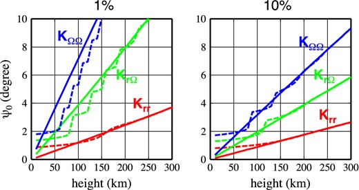
The angular distance ψ0 as a function of the computation-point height for the full-spectrum isotropic kernels Krr (red solid line), KrΩ (green solid line) and KΩΩ (blue solid line) evaluated by the closed forms (47), and for the bandwidth-limited isotropic kernels Krr (red dashed line), KrΩ(green dashed line) and KΩΩ (blue dashed line) evaluated by summing the series of Legendre polynomials (30) truncated at degree jmax = 220. The ratio between the amplitude of an isotropic kernel at the angular distance ψ0 to its maximum amplitude is δ = 1 per cent (left-hand panel) and δ = 10 per cent (right-hand panel).

For the identification of geological units in unexplored parts of the world, it is advantageous to interpret the GOCE-based gravitational gradients at lower altitudes since the gravitational gradient signals are amplified and better reflect near-surface geological structures. Since the omission error for a near-surface computation point is also significantly amplified, the forward geophysical modelling must ensure that the omission error of the forward-modelled gravitational gradients is the same as the omission error of the GOCE-based gravitational gradients. Only after this are the GOCE-based gravitational gradients able to be interpreted in terms of geological structure. One way of performing this step is to pass the forward-modelled gravitational gradients through the bandpass filter with the same bandwidth as the GOCE-based gravitational gradients (e.g. Martinec 1991). This approach has been applied by Martinec & Fullea (2013) when interpreting the GOCO03S gravity model to refine a model of sedimentary rock cover in the southeastern part of the Congo basin.

6.2 Sensitivity of the gravitational gradients to the depth of the mass anomalies

Let us express the angularly dependent part of density |$\varrho (\vec{r})$| in spherical coordinates (ψ, α) as a series of spherical harmonics,
\begin{equation} \varrho (\vec{r} =\sum _{j=0}^\infty \sum _{m=-j}^j\varrho _{jm}(r^{\prime })Y_{jm}(\psi ,\alpha ). \end{equation}
(51)
To analyse the sensitivity of the satellite gradiometric tensor to the depth of a density anomaly source, a δ-like spherical sheet with a surface density distribution of Yjm(ψ, α) is placed in the Earth's interior at radius r0,
\begin{equation} \varrho (\vec{r}^{\prime })=\sigma _0\,\delta (r^{\prime }-r_0)Y_{jm}(\psi ,\alpha ), \end{equation}
(52)
where σ0 = 1 kg m−2. Inserting this density model and eq. (31) into eq. (50), we have
\begin{eqnarray} D_{rr,jm}(r_0,r)&=&{\kappa \over r^3} \int \limits _{\psi =0}^\pi \int \limits _{\alpha =0}^{2\pi }\int \limits _{r^{\prime }} \sigma _0\,\delta (r^{\prime }-r_0)Y_{jm}(\psi ,\alpha )\nonumber \\ && \times \sum _{j_1=0}^\infty (j_1+1)(j_1+2)\sqrt{4\pi \over 2j_1+1} \bigg ({r^{\prime }\over r}\bigg )^{j_1}\nonumber \\ &&\times\,P_{j_10}(\cos \psi )(r^{\prime })^2\sin \psi \, {\rm d}r^{\prime } d\psi \, {\rm d}\alpha , \end{eqnarray}
(53)
where we have added the argument r0 and indices jm to the Drr to indicate that Drr, jm(r0, r) is the vertical-vertical gravitational gradient response (or Green's function) to a simple density anomaly of the form given by eq. (52). Making use of the sifting property of the delta function and the orthonormality property of spherical harmonics yields
\begin{equation} D_{rr,jm}(r_0,r)={\kappa \sigma _0\over r}\bigg ({r_0\over r}\bigg )^{j+2} (j+1)(j+2)\sqrt{4\pi \over 2j+1}\,\delta _{m0}. \end{equation}
(54)
The other gravitational gradient responses (50) can be arranged in a similar way, obtaining
\begin{eqnarray} \left\lbrace \begin{array}{c}D_{r\vartheta ,jm}(r_0,r) \\ D_{r\varphi ,jm}(r_0,r) \end{array} \right\rbrace ={\kappa \sigma _0\over r}\bigg ({r_0\over r}\bigg )^{j+2} (j+2)\sqrt{j(j+1)} \nonumber \\ \times\,\sqrt{4\pi \over 2j+1} \left\lbrace \begin{array}{l}(\delta _{m1}+\delta _{m,-1})\\ (-i)(\delta _{m1}-\delta _{m,-1}) \end{array} \right\rbrace \end{eqnarray}
(55)
and
\begin{eqnarray} \left\lbrace \begin{array}{c}D_{\vartheta \vartheta \varphi \varphi ,jm}(r_0,r)\nonumber \\ D_{\vartheta \varphi ,jm}(r_0,r) \end{array} \right\rbrace &=&{\kappa \sigma _0\over r}\bigg ({r_0\over r}\bigg )^{j+2} {1\over 4}\sqrt{(j-1)j(j+1)(j+2)}\nonumber \\ &&\times\,\sqrt{4\pi \over 2j+1} \left\lbrace \begin{array}{l}(\delta _{m2}+\delta _{m,-2})\\ (-i)(\delta _{m2}-\delta _{m,-2}) \end{array} \right\rbrace . \end{eqnarray}
(56)
 One way to plot the ‘D’ gravitational gradient responses is to express them relative to those for a density anomaly placed at the Earth's surface, that is for r0 = a. For instance, the normalized response for vertical-vertical gravitational gradient is
\begin{equation} {D_{rr,jm}(r_0,r)\over D_{rr,jm}(a,r)}=\bigg ({r_0\over a}\bigg )^{j+2}\,\delta _{m0}. \end{equation}
(57)
Likewise, the normalized ‘D’ response for the vertical-horizontal gravitational gradient is
\begin{equation} {D_{r\vartheta ,jm}(r_0,r)\over D_{r\vartheta ,jm}(a,r)}=\bigg ({r_0\over a}\bigg )^{j+2} \,(\delta _{m1}+\delta _{m,-1}). \end{equation}
(58)
The same ratio (r0/a) j + 2 occurs at the other three normalizes ‘D’ gravitational gradient responses. Fig. 3 plots the normalized response function (r0/a) j + 2 for harmonic degrees j = 2, 4, ⋅⋅⋅, 250. It tells us what is the amplitude of the gravitational gradient induced by an internal δ-like density anomaly as a function of the depth of the anomaly as it varies through the Earth's mantle. The largest gravitational gradient response is, naturally, obtained for shallow mass anomalies. This behaviour is further amplified as the harmonic degree increases because of the attenuation effect due to the term (r0/a) j + 2. The vertical-vertical gravitational gradient response function does not depend on the azimuthal order m, whereas the horizontal-vertical and horizontal-horizontal gravitational gradient response functions depend on m = ±1 and m = ±2, respectively. Note that the normalized response (Green's) function of the static geoid, that is the case without the gravitational contribution of boundary deflections due to mantle convection, has the same form as eq. (57) (Richards & Hager 1984).
Figure 3.

The normalized response function (r0/a) j + 2 for harmonic degrees j = 2, 4, 10, 30, 90, 150, 250.

7 SUMMARY AND CONCLUSIONS

This paper has been motivated by an effort to create an adequate mathematical tool for analysing the sensitivity of satellite gradiometric data, as provided by the GOCE mission, to the Earth's internal density structure and to the height where the GOCE-based gravitational gradients are considered. It has been shown that an approach based on Green's functions is highly convenient for carrying out such an analysis. We express the Green's functions for gravitational gradients in the spectral form as a series of tensor spherical harmonics. This form of the Green's functions can be used for representing the forward-modelled gravitational gradients when the GOCE-based gravitational gradients are interpreted at different heights above the Earth's surface. Alternatively, by means of the addition theorems for tensor spherical harmonics, the spectral forms are converted to closed spatial forms. These two alternative forms provide a powerful tool for analysing the omission error of the bandwidth-limited GOCE-based gravitational gradients at the satellite's altitude and its amplification at lower altitudes. We show that the omission error of the bandwidth-limited Green's functions for gradiometric data at the GOCE satellite altitude does not exceed 1 per cent in amplitude when compared to the full-spectrum Green's functions. Such an error may be tolerated for certain types of geophysical applications (Bouman et al.2013; Fullea et al.2013). However, when computing the bandwidth-limited gravitational gradients close to the Earth's surface, the omission error is significantly enhanced. We conclude that the GOCE-based gravitational gradients at altitudes close to the Earth's surface could be interpreted in terms of the Earth's density structure only after filtering the short-wavelength content of the forward-modelled gravitatinal gradients, such that the omission error of the GOCE-based gravitational gradients is equal to the omission error of the forward-modelled gravitational gradients.

The spectral forms of the gravitational gradients additionally allow us to calculate the sensitivity of the satellite gravitational gradients to the depth of a density anomaly, expressed in terms of the harmonic degree of the internal density anomaly. We show that the largest gravitational gradient response is obtained for shallow mass anomalies, and is further amplified as the harmonic degree increases. That is why the GOCE gravitational gradients are able to improve the modelling of the Earth's crustal and lithospheric structure. In addition, if they are evaluated near the Earth's surface, the gravitational gradient signal is amplified and better reflects the near-surface geological structure, which may be an advantage for geological mapping in less well-surveyed regions.

The author would like to thank Roger Haagmans for directing attention to the problem studied in this paper, Kevin Fleming and two anonymous reviewers for their comments on the manuscript that have helped to improve the manuscript. This work has been carried out within the framework of the ESA sponsored GOCE-GDC study and the research program 11/RFP.1/GEO/3309 financed by the Science Foundation of Ireland. The author acknowledges this support.

REFERENCES

Álvarez
O.
Gimenez
M.
Braitenberg
C.
Folguera
A.
GOCE satellite derived gravity and gravity gradient corrected for topographic effect in the South Central Andes region
Geophys. J. Int.
2012
, vol. 
190
 (pg. 
941
-
959
)
Arfken
G.
Mathematical Methods for Physicists
1968
Academic Press
Ballani
L.
Engels
J.
Grafarend
E.W.
Global base functions for the mass density in the interior of a massive body (Earth)
Manusc. Geod.
1993a
, vol. 
18
 (pg. 
99
-
114
)
Ballani
L.
Stromeyer
D.
Barthelmes
F.
Anger
G.
Gorenflo
R.
Jochmann
H.
Moritz
H.
Webers
W.
Decomposition principles for linear source problems
Inverse Problems: Principles and Applications in Geophysics, Technology and Medicine
1993b
Akademie Verlag
(pg. 
45
-
59
)
Bingham
R.
Knudsen
P.
Andersen
O.
Pail
R.
An initial estimate of the North Atlantic steady state geostrophic circulation from GOCE
Geophys. Res. Lett.
2011
, vol. 
38
 pg. 
L01606
  
doi:10.1029/2010GL045633
Bölling
C.
Grafarend
E.W.
Ellipsoidal spectral properties of the Earths gravitational potential and its first and second derivatives
J. Geod.
2005
, vol. 
79
 (pg. 
300
-
330
)
Bouman
J.
Fuchs
M.J.
GOCE gravity gradients versus global gravity field models
Geophys. J. Int.
2012
, vol. 
189
 (pg. 
846
-
850
)
Bouman
J.
Fiorot
S.
Fuchs
M.
Gruber
T.
Schrama
E.
Tscherning
C.C.
Veicherts
M.
Visser
P.
GOCE gravitational gradients along the orbit
J. Geod.
2011
, vol. 
85
 (pg. 
791
-
805
)
Bouman
J.
, et al. 
GOCE gravity gradient data for lithospheric modeling
Int. J. Appl. Earth Obs. Geoinf.
2013
 
in press
Braitenberg
C.
Mariani
P.
Ebbing
J.
Šprlák
M.
van Hinsbergen
D.J.J.
Buiter
S.J.H.
Torsvik
T.H.
Gaina
C.
Webb
S.J.
The enigmatic Chad lineament revisited with global gravity and gravity gradient fields
The Formation and Evolution of Africa: A Synopsis of 3.8 Ga of Earth History
2011
Geological Society, Special Publications
(pg. 
329
-
341
Vol 357
Eshagh
M.
The effect of spatial truncation error on the integral inversion of satellite gravity gradiometry data
Adv. Space Res.
2011
, vol. 
47
 (pg. 
1238
-
1247
)
Frommknecht
B.
Lamarre
D.
Meloni
M.
Bigazzi
A.
Floberghagen
R.
GOCE level 1b data processing
J. Geod.
2011
, vol. 
85
 (pg. 
759
-
775
)
Fullea
J.
Fernàndez
M.
Zeyen
H.
FA2BOUG-a FORTRAN 90 code to compute Bouguer gravity anomalies from gridded free air anomalies: application to the Atlantic-Mediterranean transition zone
Comput. Geosci.
2008
, vol. 
34
 (pg. 
1665
-
1681
)
Fullea
J.
Rodríguez-González
J.
Charco
M.
Martinec
Z.
Negredo
A.
Villaseñor
A.
Upper mantle structure under the Atlantic-Mediterranean transition zone: new constraints from GOCE mission and other potential field data
Int. J. Appl. Earth Obs. Geoinf.
2013
 
submitted
Grafarend
E.
The spherical horizontal and spherical vertical boundary value problem—vertical deflections and geoidal undulations—the completed Meissl diagram
J. Geod.
2001
, vol. 
75
 (pg. 
363
-
390
)
Grombein
T.
Seitz
K.
Heck
B.
Optimized formulas for the gravitational field of a tesseroid
J. Geod.
2013
, vol. 
87
 (pg. 
645
-
660
)
Hadamard
J.
Lectures on Cauchy's Problem in Linear Partial Differential Equations
1923
Yale University Press
Heiskanen
W.A.
Moritz
H.
Physical Geodesy
1967
Freeman & Co
Hirt
C.
Kuhn
M.
Featherstone
W.E.
Göttl
F.
Topographic/isostatic evaluation of new-generation GOCE gravity field models
J. geophys. Res.
2012
, vol. 
117
 pg. 
B05407
  
doi:10.1029/2011JB008878
Kellogg
O.D.
Foundations of Potential Theory
1954
Dover Press
Köther
N.
, et al. 
The seismically active Andean and Central American margins: can satellite gravity map lithospheric structures?
J. Geodyn.
2012
, vol. 
59
 (pg. 
207
-
218
)
Losch
M.
Sloyan
B.M.
Schröter
J.
Sneeuw
N.
Box inverse models, altimetry and the geoid: problems with the omission error
J. geophys. Res.
2002
, vol. 
107
 (pg. 
15-1
-
15-13
)
Mariani
P.
Braitenberg
C.
Ussami
N.
Explaining the thick crust in Paraná basin, Brazil, with satellite GOCE gravity observations
J. South Am. Earth Sci.
2013
, vol. 
45
 (pg. 
209
-
223
)
Martinec
Z.
Program to calculate the least-squares estimates of the spherical harmonic expansion coefficients of an equally angular-gridded scalar field
Comput. Phys. Comm.
1991
, vol. 
64
 (pg. 
140
-
148
)
Martinec
Z.
Spectral–finite element approach to three-dimensional viscoelastic relaxation in a spherical earth
Geophys. J. Int.
2000
, vol. 
142
 (pg. 
117
-
141
)
Martinec
Z.
Green's function solution to spherical gradiometric boundary-value problems
J. Geod.
2003
, vol. 
77
 (pg. 
41
-
49
)
Martinec
Z.
Fullea
J.
A refined model of sedimentary rock cover in the southeastern part of the Congo basin from GOCE gravity and vertical gravity gradient observations
Int. J. Appl. Earth Obs. Geoinfor.
2013
 
submitted
Matyska
C.
The inverse gravimetric problem: existence, uniqueness and stability of the solution
Studia Geophys. et Geod.
1987
, vol. 
31
 (pg. 
252
-
257
)
Mayer-Gürr
T.
, et al. 
The new combined satellite only model GOCO03S
Proceedings of International Symposium on Gravity, Geoid and Height Systems (GGHS’12)
2012
Venice
Meissl
P.
A study of covariance functions related to the Earth's disturbing potential. Tech. Rep. No. 151, Ohio State University, Department of Geodetic Science and Surveying, Columbus, Ohio
1971
Menke
W.
Geophysical Data Analysis: Discrete Inverse Theory
1989
2nd edn
Academic Press
Pail
R.
Fecher
T.
Murböck
M.
Rexer
M.
Stetter
M.
Gruber
Th.
Stummer
C.
Impact of GOCE Level 1b data reprocessing on GOCE-only and combined gravity field models
Studia Geophysica et Geodaetica
2013
, vol. 
57
 (pg. 
155
-
173
)
Parker
R.L.
Geophysical Inverse Theory
1994
Princeton Univ. Press
Pavlis
N.K.
Holmes
S.A.
Kenyon
S.C.
Factor
J.K.
The development and evaluation of the Earth Gravitational Model 2008 (EGM2008)
J. geophys. Res.
2012
, vol. 
117
 pg. 
B04406
  
doi:10.1029/2011JB008916
Pěč
K.
Martinec
Z.
Constraints to three dimensional non-hydrostatic density distribution in the Earth
Studia Geoph. et Geod.
1984
, vol. 
28
 (pg. 
364
-
380
)
Renardy
M.
Rogers
R.C.
An Introduction to Partial Differential Equations
1993
Texts in Applied Mathematics, Springer-Verlag
Richards
M.A.
Hager
B.A.
Geoid anomalies in a dynamic Earth
J. geophys. Res. Solid Earth
1984
, vol. 
89
 (pg. 
5987
-
6002
)
Rummel
R.
van Gelderen
M.
Meissl scheme—spectral characteristics of physical geodesy
Manuscripta Geodaetica
1995
, vol. 
20
 (pg. 
379
-
385
)
Rummel
R.
Yi
W.
Stummer
C.
GOCE gravitational gradiometry
J. Geod.
2011
, vol. 
85
 (pg. 
777
-
790
)
Sansò
F.
Barzaghi
R.
Tscherning
C.C.
Choice of norm for the density distribution of the Earth
Geophys. J. R. astr. Soc.
1986
, vol. 
87
 (pg. 
123
-
141
)
Tarantola
A.
Inverse Problem Theory and Methods for Model Parameter Estimation
2005
SIAM
Tsoulis
D.
Analytical computation of the full gravity tensor of a homogeneous arbitrarily shaped polyhedral source using line integrals
Geophysics
2012
, vol. 
77
 (pg. 
F1
-
F11
)
Uieda
L.
Bomfim
E.
Braitenberg
C.
Molina
E.
Optimal forward calculation method of the Marussi tensor due to a geologic structure at GOCE height
Proceedings of GOCE User Workshop 2011
2011
 
ESA SP-696
Varshalovich
D.A.
Moskalev
A.N.
Khersonskii
V.K.
Quantum Theory of Angular Momentum
1989
World Scientific Press
Xu
P.
Truncated SVD methods for discrete linear ill-posed problems
Geophys. J. Int.
1998
, vol. 
135
 (pg. 
505
-
514
)