


Abstract
Both rupture and wave propagation affect strong ground motions on the surface. The complexity of finite earthquake source process plays a significant role in determining near-source ground motion characteristics, especially for large events. Spontaneous dynamic rupture modelling has great potential to study ground motions dominated by earthquake source and has been efficiently adopted for physics-based source and ground motion modelling for the last several decades, but the input of the state of initial stress, friction laws and their parametrization are still not well constrained in general. We demonstrate that at least two statistical measures, that is 1-point and 2-point statistics, are needed to quantify the heterogeneity of spatial data and that 1-point statistics such as mean, standard deviation and shape of probability density function of dynamic input parameters, is a separate quantity that we need to consider in addition to 2-point statistics in earthquake source modelling. We show that 1-point statistics of input dynamic parameters such as stress drop can significantly affect resulting kinematic source and near-source ground motions. The standard deviations of input stress drop affect both 1-point and 2-point statistics of kinematic source parameters derived from spontaneous rupture modelling significantly and even systematically. They also strongly control near-source ground motions, especially in the rupture directivity region. Quantifying the characteristics of both earthquake source and ground motions in the same format of 1-point and 2-point statistics may help us to construct a consistent framework for studying the effect of finite earthquake source process on near-source ground motions.
1 INTRODUCTION
Finite earthquake rupture process can affect near-source ground motion characteristics significantly, especially if rupture dimension is relatively large compared to source-to-site distance. Both kinematic and dynamic source modelling have been extensively used to study earthquake phenomena for a better understanding of earthquake source process on near-source ground motion characteristics. Kinematic modelling, in which the spatiotemporal evolution of the source slip function is a priori assumed, benefits from its computational efficiency and it may have better observational constraints (Graves et al.2011). Dynamic modelling spontaneously determines the complex spatiotemporal evolution of earthquake rupture, based on applied stress fields and friction laws, thus it may provide physical self-consistency to resulting kinematic source motions (Guatteri et al.2003; Olsen et al.2009). The physical framework adopted in dynamic modelling also enables us to investigate the effect of specific physical aspects of rupture process on ground motions, such as supershear/subshear rupture and surface/buried rupture (Bizzarri & Spudich 2008; Dalguer et al.2008; Pitarka et al.2009; Bizzarri et al.2010). There also have been valuable efforts to combine strengths from both dynamic and kinematic modelling approaches and to develop optimal source modelling methods (Guatteri et al.2004; Schmedes et al.2010; Song & Somerville 2010; Mena et al.2012).
Whether it is dynamic or kinematic source modelling, it is very challenging to simulate the spatial heterogeneity of relevant source parameters on a finite fault plane, which also have poor observational constraints so far. The spatial distribution of stress drop and final slip is often modelled by specifying their spectral decay pattern in the Fourier domain (Andrews 1980; Mai & Beroza 2002; Ripperger et al.2007; Bizzarri 2010; Graves & Pitarka 2010; Andrews & Barall 2011). According to the autocorrelation theorem (Bracewell 2000, pp. 122–124), the Fourier spectrum controls the 2-point autocorrelation structure of source parameters. 1-point statistics of source parameters is, however, often not explicitly considered in the Fourier transform-based source modelling approaches although recently there are few attempts to constrain 1-point statistics and to test its effect on the development of rupture processes (Lavallee & Archuleta 2003; Lavallee et al.2006; Liu et al.2006; Hillers et al.2007; Ripperger et al.2007). To our knowledge, the importance of 1-point statistics in earthquake source modelling and, in particular, its effect on near-source ground motions has not been well studied in a systematic sense.
In this study, we claim that at least two statistical measures, that is 1-point and 2-point statistics, are needed to quantify the heterogeneity of spatial data. 1-point statistics such as mean, standard deviation, and the shape of probability density function (PDF) of earthquake source parameters at a given point on the fault, is a separate quantity that needs to be considered and constrained in addition to 2-point statistics, that is 2-point spatial correlation. We also introduce spatial random field model as an alternative source modelling approach in addition to the Fourier transform-based ones, in which the concept of 1-point statistics may be embodied in a more natural way. Taking into account 1-point statistics of source parameters explicitly in dynamic rupture modelling, we demonstrate that resulting kinematic source and near-source ground motions can be significantly and even systematically affected by the 1-point statistics of input source parameters. Finally, this study suggests that we may construct a consistent framework to study the effect of earthquake source process on near-source ground motions by quantifying the characteristics of both earthquake source and ground motions in the same format of 1-point and 2-point statistics.
2 HETEROGENEITY OF SPATIAL DATA
2.1 Random realization with power spectral density (PSD)
Random spatial distributions can be easily simulated with a specified spectral decay rate in the Fourier amplitude spectrum (Andrews 1980; Andrews & Barall 2011). Once the spectral decay rate is determined as a function of wavenumber, for example k−1, combining them with a random phase spectrum and taking the inverse Fourier transform will generate random spatial distributions of a target source parameter. Although each individual distribution may vary randomly in the spatial domain, all distributions are supposed to share the same target spectral decay rate. And it is the random phase spectrum that introduces randomness in the generated spatial distributions. However, it is important to note that randomly realized spatial distributions can vary significantly, depending on how to combine amplitude spectrum with phase spectrum. For example, we can combine the amplitude spectrum not only with a uniformly distributed random phase spectrum, but also a constant zero phase spectrum. Although the uniformly distributed phase spectrum is conventionally used in earthquake source modelling, it is not clear whether it has a physical basis and whether it is a unique way of characterizing the phase spectrum in the Fourier transform-based random realizations.
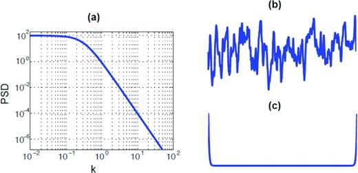
(a) Power spectral density (PSD) given in eq. (1), (b) an example of 1-D random realization obtained by combining the amplitude spectrum from the PSD in (a) with a uniformly distributed random phase spectrum, (c) an example of 1-D random realization with the same PSD used in (b), but with a constant phase spectrum that contains only zero phases.
Eq. (2) clearly indicates that the perturbation of standard deviation in a heterogeneous spatial distribution does not change the spectral decay rate of the Fourier amplitude spectrum in a log–log plot as shown in Fig. 2. In other words, different standard deviations only move the whole PSD curve in a vertical direction without changing the shape of the spectral decay pattern. The 1-D spatial realization in green in Fig. 2(a) is obtained by standardizing the 1-D spatial realization in Fig. 1(b). The blue and red traces are obtained by multiplying the green trace by a factor of 2 and 3, respectively. Note that the contribution from mean, μ, would not appear in Fig. 2(c), even though it has a non-zero value, because this term becomes zero where k has non-zero values. If we consider a heterogeneous earthquake slip distribution, we can easily demonstrate that the mean slip (or seismic moment) does not determine the PSD amplitude of the heterogeneous slip distribution where k has non-zero values, but the standard deviation of earthquake slip does.
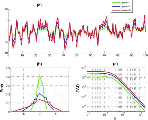
(a) Three sets of 1-D spatial data obtained from Fig. 1b. They have the same zero means, but different standard deviations, (b) empirical 1-point probability density functions obtained from the three traces in (a), (c) PSD curves obtained from the three spatial data in (a). Note that the shape of spectral decay pattern is preserved although the whole PSD curve moves up and down, depending on the amount of standard deviations as given in eq. (2).
The transformation of 1-point statistics in Fig. 2(b), preserving the shape of PDF (Gaussian distribution in this case), only perturbs the standard deviation. However, the shape of the PDF of 1-point statistics can also be perturbed easily using the inverse transform method (see Appendix A for details). It is also worthy to remember that in general the Fourier amplitude spectrum is not distorted even after the shape of 1-point PDF is changed, that is from a Gaussian distribution to a non-Gaussian distribution, as demonstrated in Fig. 3. Fig. 3(a) shows three different 1-D spatial distributions. Two traces following Uniform (blue) and Exponential (red) distributions are obtained by the inverse transform method from the trace in green that follows the Gaussian distribution and resulting 1-point PDFs are shown in Fig. 3(b). Their mean and standard deviation are adjusted to have the same zero mean and unit standard deviation. Fig. 3(c) clearly shows that the transform of 1-point statistics from a Gaussian to a non-Gaussian distribution does not distort their spectral decay rate. In general it is expected to be true as long as the transform function, that is the cumulative density function (CDF) of transformed distribution, is smoothly and monotonically increasing.
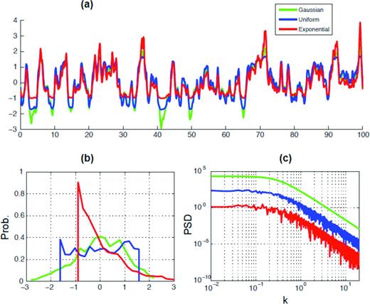
(a) Three sets of 1-D spatial data following different 1-point probability density functions. Two traces in blue and red are obtained by the inverse transform method from the green trace (see Appendix A for details), (b) empirical 1-point probability density functions obtained from the three traces in (a), (c) PSD curves obtained from the three spatial traces in (a). The oscillations observed in blue and red traces are considered numerical noises introduced by the inverse transform method. All three PSDs are originally aligned on top of one another because they have the same standard deviation, but they are shifted in the vertical direction for visualization purposes only.
2.2 Random realization with spatial random field
Although the Fourier transform-based random realization is well adopted in earthquake source modelling, we can perform a similar kind of realization with a spatial random field model as well. In the framework of a spatial random field model we can actually introduce the concept of 1-point statistics more naturally. The crosscorrelation structures that may be embedded between different source parameters, as introduced by Song et al. (2009) and Song & Somerville (2010), can also be implemented in a more consistent way. Fig. 4 shows an example of spatial random field model implemented in the spatial data of earthquake source parameters. Earthquake rupture can be modelled by a set of spatial distributions of source parameters. In dynamic modelling, they may be stress drop and fracture energy, etc. In kinematic modelling, they may be composed of a set of kinematic parameters, such as slip, rupture velocity, slip velocity and duration. In a spatial random field model, we assign random field, {X(uij), i = 1,…,M, j = 1,…,N}, to one source parameter such as earthquake slip and random field, {Y(uij), i = 1,…,M, j = 1,…,N}, to another source parameter such as rupture velocity, and so on. M and N are the number of subfault elements in the along-dip and along-strike directions, respectively. The random field (or random function) is nothing but a set of random variables. For instance, the random field, {X(uij), i = 1,…,M, j = 1,…,N}, is composed of M × N random variables where uij is a location vector that is linked to an individual subfault patch. If a faulting plane is not discretized, we can consider a continuous random field model, {X(u), ∀u∈ A}, where A indicates a faulting area. However, the discrete random field model, {X(uij), i = 1,…,M, j = 1,…,N}, is used in our study. We also prefer using the term, ‘random field’, instead of ‘random function’ because we deal with 2-D spatial data on a finite faulting plane.
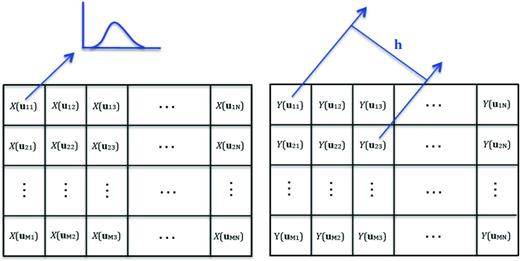
Spatial distribution of random variables assigned to each source parameter on a planar fault, that is X(uij) and Y(uij) are random variables that represent one of source parameters such as stress drop and final slip, rupture velocity, etc. uij is a location vector and h is a separation vector between two random variables. Random variables, X and Y, have their own univariate (1-point) probability density function (PDF) at a given subfault patch, and 2-point correlation structures can also be inferred as a function of h.
If we have two different source parameters, each has M × N random variables, that is M ×N subfault patches on a faulting plane, in principle we need a complete form of 2(M × N)-dimensional multivariate PDF to characterize the random field model. Simply drawing samples following the target PDF with a certain kind of Monte Carlo sampling method can produce a large number of random spatial distributions of target source parameters. However, in most practical applications, this level of statistical inference is almost impossible. In practice, we are often limited to constraining their 1-point statistics and 2-point correlation structures. However, it is important to note that this framework actually provides more constraints to spatial data than the Fourier amplitude spectrum-based approach. In other words, the PSD is directly linked to 2-point autocorrelation, based on the autocorrelation theorem (Bracewell 2000) and 1-point statistics and 2-point crosscorrelation can serve as additional constraints to random spatial data simulation.
2.2.1 1-point statistics
1-point statistics of earthquake source parameters has not been intensively studied in earthquake seismology, compared to 2-point autocorrelation (or spectral decay in PSD) addressed in the Section 2.2.2. Lavallee & Archuleta (2003) and Lavallee et al. (2006) tried to constrain 1-point variability of earthquake slip from kinematic rupture models. Lavallee & Archuleta (2005) and Causse et al. (2010) also tried to link 1-point variability of earthquake slip with 1-point variability of ground motion intensity parameters. However, given the fact that predicting 1-point statistics (e.g. median and sigma) of ground motion intensity parameters such as peak ground velocity (PGV) and spectral acceleration (SA) is one of primary interests in earthquake source modelling, we may need to pay more attention to 1-point statistics of earthquake source parameters. In this paper, we demonstrate that near-source ground motions can be affected significantly by 1-point statistics of source parameters.
2.2.2 2-point statistics
CovXX (h) and CovXY (h) are called auto- and crosscovariance function, respectively, and their normalized quantities, that is ρXX (h) = CovXX (h) / σX2 and ρXY (h) = CovXY (h) / (σXσY), are called auto- and crosscorrelogram (Goovaerts 1997). σX and σY are standard deviations for random variables, X(uij) and Y(uij), respectively. ρXX (h) and ρXY (h) can be inferred from spatial data of source parameters [see eqs (1)–(5) in Song & Somerville (2010)].
Autocorrelation: autocorrelogram, ρXX(h) = CovXX(h)/σ2X, controls correlation structure within a single kind of spatial data, that is spatial continuity or discontinuity of stress drop or earthquake slip, etc. According to the autocorrelation theorem (Bracewell 2000), if the function, f(x), has the Fourier transform, F(k), then its autocorrelation function (ACF) has the Fourier transform, |F(k)|2, which is the PSD of f(x). Because autocorrelogram, ρXX(h), has an equivalent functional form to the ACF [see eqs (1) and (2) in Song & Somerville (2010)], the autocorrelogram is directly linked to PSD and the PSD is one kind of measure of 2-point autocorrelation structure. Both ρXX(h) and ρXY(h) vary between −1 and 1. The 2-point autocorrelation of earthquake slip has been extensively studied in earthquake seismology in the context of spectral decay in PSD (Andrews 1980; Herrero & Bernard 1994; Somerville et al.1999; Mai & Beroza 2002; Lavallee & Archuleta 2003; and references therein).
Crosscorrelation: cross-correlogram, ρXY(h) = CovXY(h)/(σXσY), controls correlation structures between different source parameters. Correlations between source parameters are important in association with physics-based kinematic source modelling (Guatteri et al.2004; Schmedes et al.2010; Song & Somerville 2010; Mena et al.2012). Arbitrary non-physical combinations of source parameters can be prevented in kinematic source modelling with appropriate crosscorrelation structures. Several interesting features of earthquake rupture have been found by investigating crosscorrelation structure of both kinematic and dynamic rupture models (Song et al.2009; Song & Somerville 2010). For instance, the correlation maximum between slip and rupture velocity can be shifted from zero offset, that is large slip may generate faster rupture velocity ahead of the current rupture front, which may be an important element in association with rupture directivity. Because the ACF does not have any phase information, it is directly linked to the Fourier amplitude spectrum, but the crosscorrelation function may still have phase information such as the offset of crosscorrelation maximum, which cannot be well modelled with the Fourier amplitude spectrum only. This is one of the main reasons that we prefer investigating the coupling of spatial data between different source parameters using the statistical term, crosscorrelogram, in the framework of a spatial random field model.
In summary, we claim that realization of spatial data with a random field model have advantages over the Fourier amplitude spectrum-based approaches. First, the concept of 1-point statistics is more naturally introduced in this way, and secondly the crosscorrelation between different types of spatial data, for example between rupture velocity and peak slip velocity, is also handled in a consistent way with the autocorrelation within a single type of data.
3 DYNAMIC SOURCE MODELLING WITH 1-POINT AND 2-POINT STATISTICS
Earthquake rupture is a physical process that is governed by applied stress and friction laws on the discontinuous interface, that is fault, embedded inside the brittle rock of the Earth, which can be efficiently modelled by dynamically running crack propagation (Andrews 1976; Day 1982). This type of dynamic rupture modelling has been well adopted by numerous researchers to understand the physics of rupture processes and also for physics-based ground motion modelling. However, input stress and friction parameters are not well constrained in general in dynamic modelling, which limits the full efficiency of dynamic modelling in earthquake source and ground motion studies. Because of the heterogeneous nature of earthquake source, stochastic characterization of input dynamic parameters appears to be the most reasonable way of studying earthquakes and resulting ground motions (e.g. Ampuero et al.2006; Ripperger et al.2008; Mena et al.2012). In this paper, we aim to formulate the characteristics of finite faulting in the framework of 1-point and 2-point statistics introduced in Section 2, and to investigate the effect of 1-point statistics, in particular 1-point statistics of input stress drop, on resulting kinematic source and near-source ground motions. Although constraining 1-point statistics of source parameters is beyond the scope of this paper, we hope that this type of forward modelling study draws attention to the importance of 1-point statistics in earthquake source modelling and motivates researchers to constrain the 1-point statistics in various ways.
3.1 1-point and 2-point statistics in dynamic source
Independent of the absolute values of initial stress and frictional strengths, the state of the stress field for dynamic rupture models can be characterized in terms of the dimensionless ratio, S = SE/Δσ, as introduced by Andrews (1976), which is a measure of how close the initial stress field is to failure. SE is the strength excess, which is a measure of the static yielding strength minus the initial stress, and Δσ is the dynamic stress drop (hereafter ‘stress drop’), which is a measure of the initial stress minus the dynamic yielding strength. In addition, the energy flux into the crack tip (so called fracture energy, Gc) that plays an important role in earthquake dynamics can also be parametrized for dynamic rupture simulations. Under the slip weakening friction law (Andrews 1976), strength excess (SE), stress drop and the slip weakening distance (Dc) determine the fracture energy. This set of parameters complete the dynamic rupture parametrization. These dynamic parameters are not well constrained in general, although average stress drop and fracture energy can be estimated by seismological methods. The fracture energy estimation is considered less robust (e.g. Abercrombie & Rice 2005).
Because among all parameters, stress drop is better constrained with observations, here we focus on the statistical properties of stress drop and their effect on the resulting kinematic source and near-source ground motion, leaving the other parameters for future studies. The spatial heterogeneity of stress drop is often modelled with a spectral decay model such as k−1 (Andrews 1980; Andrews & Barall 2011) although its 1-point statistics is often not explicitly addressed. We adopt the same (k−1) spectral decay model for the 2-point autocorrelation structure of stress drop, but perturb its 1-point statistics systematically and carefully examine how it affects resulting kinematic source and near-source ground motions.
Fig. 5 shows three simulated stress drop distributions. They all follow the same k−1 spectral decay rate and share the same Gaussian 1-point PDF with the same mean stress drop (=3 MPa), the only varying parameter is standard deviation, which varies from 1 MPa (a) to 3 MPa (c). Relevant statistical measures are presented in Fig. 6. Fig. 6(a) confirms that all three distributions follow the same Gaussian 1-point statistics with different standard deviations. Fig. 6(b) verifies that their spectral decay rates are not perturbed by the different standard deviations. However, as illustrated in Fig. 5, larger standard deviations lead to higher peaks and lower troughs locally in the input stress drop, which may affect dynamic rupture propagations on the fault and possibly near-source ground motion characteristics. As explained in Appendix A, the shape of 1-point statistics can also be changed by the inverse transform method from a Gaussian distribution to a non-Gaussian distribution. More importantly, this transform does not perturb the 2-point autocorrelation structure (i.e. spectral decay rate) in general. Fig. 7 shows the uniform stress drop distribution transformed from the Gaussian 1-point statistics with the original Gaussian distribution. Fig. 8 verifies that the transform does not perturb the spectral decay rate. Thus, two distributions in Fig. 7 share the same 2-point autocorrelation structure (k−1) and the same mean (=3 MPa) and standard deviation (=2 MPa), but different shapes of 1-point PDF, that is Gaussian (Fig. 7a) and Uniform (Fig. 7b). The distributions of input stress drop with standard deviation 1 and 3 MPa are provided in Figs S1 and S2, respectively.
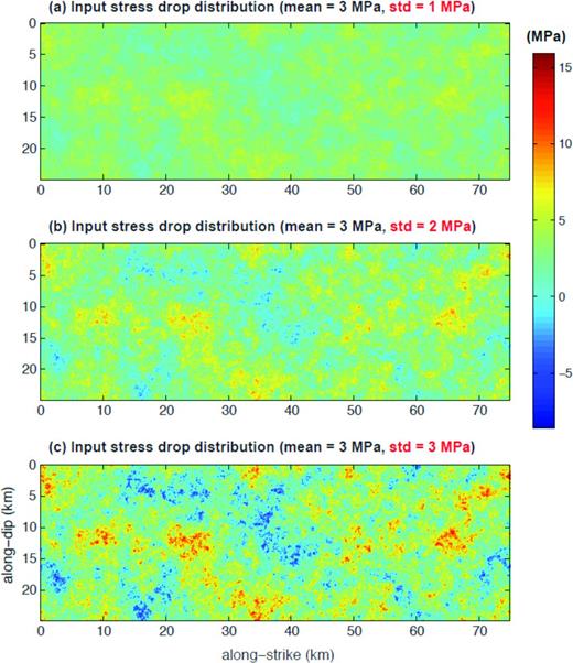
Input stress drop distribution with the same Gaussian 1-point statistics, but different standard deviations, that is (a) 1 MPa, (b) 2 MPa, (c) 3 MPa. All three distributions have the same mean stress drop (=3 MPa) and follow the same spectral decay rate (k−1).
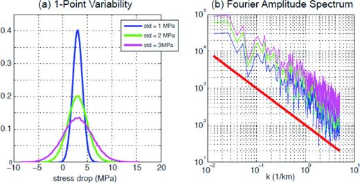
1-point probability density function (a) and Fourier amplitude spectrum (b) of three input stress drop distributions in Fig. 5. Note that they all have the same spectral decay rate (k−1) although the standard deviation varies from 1 to 3 MPa. The red solid line in (b) shows a reference spectral decay rate (k−1).
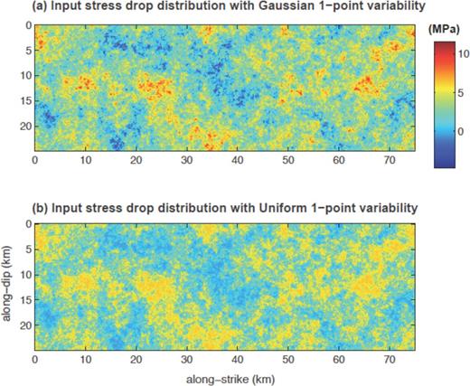
Input stress drop distributions with the Gaussian (a) and Uniform (b) 1-point statistics. Both distributions have the same mean stress drop (=3 MPa), standard deviation (=2 MPa) and spectral decay rate (=k−1).
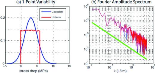
1-point statistics (a) and Fourier amplitude spectrum (b) of two input stress drop distributions in Fig. 7. Note that both have the same spectral decay rate (k−1) as shown in (b) although the shapes of their 1-point PDFs are different. The green solid line in (b) shows a reference spectral decay rate (k−1).
We also need to define the distributions of slip weakening distance (Dc) and SE as additional input parameters in our dynamic modelling. Because our primary objective in this paper is to investigate the effect of 1-point statistics of stress drop, we adopted a simplified model for both parameters, that is a constant SE (=4.5 MPa) and constant slip weakening distance (=0.25 m) for the entire rupture area. This leads to the average ratio of S = 1.5. The effect of the heterogeneity of these input parameters should also be investigated in following studies. Vertical strike-slip events are assumed and surface rupture is prohibited by putting the top edge of the faulting plane at 3 km depth. In addition, the faulting plane is embedded in a homogeneous half-space to simplify the problem. Relevant input parameters used in the modelling are summarized in Table 1. Rupture initiates in a circular nucleation patch of radius 4.0 km, located in the left side of the fault at 12.5 km from the top of the fault. In this nucleation patch, SE is set to be negative with amplitude of 5 per cent of the initial stress drop. This artificial nucleation provides the initial excitation needed to make rupture propagates spontaneously through the fault area, following the linear slip-weakening fracture criterion.
Model parameters used in dynamic modelling.
| Mean stress drop | 3 MPa |
| Strength excess (SE) | 4.5 MPa |
| Slip weakening distance (Dc) | 0.25 m |
| Grid spacing | 0.1 km |
| Time step | 0.008 s |
| P-wave speed | 6.00 km s−1 |
| S-wave speed | 3.46 km s−1 |
| Density | 2.67 g cm−3 |
| HTopa | 3 km |
| Rupture length/width | 75 km/25 km |
| Mean stress drop | 3 MPa |
| Strength excess (SE) | 4.5 MPa |
| Slip weakening distance (Dc) | 0.25 m |
| Grid spacing | 0.1 km |
| Time step | 0.008 s |
| P-wave speed | 6.00 km s−1 |
| S-wave speed | 3.46 km s−1 |
| Density | 2.67 g cm−3 |
| HTopa | 3 km |
| Rupture length/width | 75 km/25 km |
aDepth to the top of fault from the surface.
The Support Operator Rupture Dynamics code (SORD) developed by Ely et al. (2010) was used. The SORD algorithm solves the 3-D viscoelastodynamic equations of motion, coupled to frictional sliding for dynamic rupture propagation. The method uses the split-node technique for the fault representation (Day et al.2005; Dalguer & Day 2007). The code is parallelized, using Message Passing Interface, and is highly scalable, enabling large-scale earthquake simulations. Simulations are developed in a computational domain of 3008 × 344 × 4000 grid elements using 4096 processors in the high performance-computing environment of Cray XT5 Rosa Supercomputer at the Swiss National Supercomputing Center (CSCS).
3.2 1-point and 2-point statistics in kinematic source
As described early in the paper, in the dynamic rupture modelling the physical basis involved in the fault rupture is considered by introducing the causative initial stress and frictional strength. Consequently, the spatiotemporal evolution of the rupture process is determined in a physics-based way. This is the main reason why we consider the resulting kinematic source motions as physically self-consistent kinematic representation of the source rupture. Fig. 9 shows kinematic source motions on the fault in terms of slip, rupture time, and peak slip velocity obtained by spontaneous dynamic rupture modelling from three different stress drop distributions shown in Fig. 5. First of all, all three models produce the same size earthquakes (Mw 7.3) because they have the same mean stress drop (=3 MPa) and rupture area (length = 75 km, width = 25 km), but we can observe that the different standard deviations of input stress drop affect the detailed distributions of source parameters. Both slip and peak slip velocity are getting rougher as the standard deviation increases. The rupture time contour also gets perturbed more with the increasing standard deviation. These characteristics are more quantitatively measured in terms of 1-point and 2-point statistics in Figs 10 and 11. Kinematic source parameters in Fig. 9 are low-pass filtered with a minimum wavelength of 1 km. The artificial nucleation patch and small areas along the fault boundary where rupture arresting is also artificial are excluded for the computation of 1-point and 2-point statistics shown in Figs 10 and 11. Fig. 10 shows that 1-point PDFs with larger standard deviation in input stress drop have heavier tails in the upper bound. The shape of the upper tail distribution of earthquake source parameters is an important problem especially because it may dominantly control peak ground motions in a near-source region. In other words, the large slip (2.5–3 m) and large peak slip velocity (5–7 m sec–1) produced by the large standard deviation of input stress drop (=3 MPa), which are not observed in the modelling with the small standard deviation (=1 MPa), may create stronger ground motions in the near-source region. Thus it is interesting to observe the systematic push-up of the upper tail distributions of kinematic source parameters with the increasing standard deviation of input stress drop.
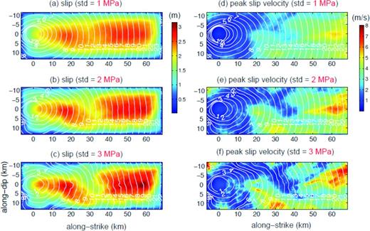
Kinematic rupture motions obtained from spontaneous dynamic rupture modelling with the slip weakening friction law with different standard deviations of input stress drop shown in Fig. 5. Final slip is plotted on the left with rupture time while peak slip velocity is plotted on the right with the same rupture time. We can easily observe that rupture front is more distorted and both slip and peak slip velocity have rougher distributions as we increase the standard deviation.
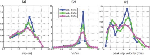
Empirical 1-point PDFs for three kinematic source parameters produced by dynamic rupture modelling, (a) final slip, (b) rupture velocity and (c) peak slip velocity. As the standard deviation increases, the upper tails of three parameters also increase.
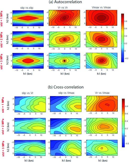
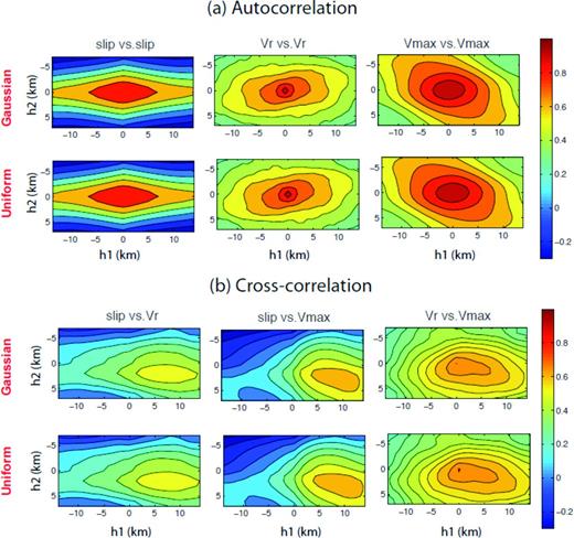
Auto (a) and crosscorrelation (b) structures for three kinematic source parameters in Fig. 9.
The measures of 2-point statistics (both auto- and crosscorrelation) show even more interesting results. Fig. 11(a) shows that the autocorrelation of the three kinematic source parameters decays faster with separation distance if the standard deviation of input stress drops increases. This pattern is relatively insignificant in earthquake slip, but it is clearly observed in temporal source parameters. Also note the anisotropic decay of autocorrelation in the along-strike and along-dip directions although the input stress drop has an isotropic spectral decay in both directions. It is interesting and also encouraging to see clear crosscorrelation structures for all three pairs, that is slip versus rupture velocity (Vr), slip versus peak slip velocity (Vmax), and rupture velocity (Vr) versus peak slip velocity (Vmax), irrespective of assigned standard deviations as shown in Fig. 11(b). In addition, correlation maximum points are shifted in the forward rupture direction up to 12 km, which are consistent with findings by Song et al. (2009) and Song & Somerville (2010). Both crosscorrelation maximum and response distance estimates decrease in general as the standard deviation increases as summarized in Table 2. It is important to understand what controls the crosscorrelation structure between kinematic source parameters because it may be a key element in physics-based kinematic source modelling for ground motion simulation. This study does not cover this issue in a comprehensive way, but the standard deviation of input stress drop may be one of the key elements that affect crosscorrelation between kinematic source parameters.
Maximum crosscorrelation coefficients and response distance (RD).
| Slip versus Vr | Slip versus Vmax | Vr versus Vmax | |
|---|---|---|---|
| Std = 1 MPa | 0.58/10.2 km | 0.63/12.2 km | 0.80/5.1 km |
| Std = 2 MPa | 0.57/7.3 km | 0.66/8.2 km | 0.70/0.0 km |
| Std = 3 MPa | 0.50/6.3 km | 0.57/7.3 km | 0.63/0.0 km |
| Slip versus Vr | Slip versus Vmax | Vr versus Vmax | |
|---|---|---|---|
| Std = 1 MPa | 0.58/10.2 km | 0.63/12.2 km | 0.80/5.1 km |
| Std = 2 MPa | 0.57/7.3 km | 0.66/8.2 km | 0.70/0.0 km |
| Std = 3 MPa | 0.50/6.3 km | 0.57/7.3 km | 0.63/0.0 km |
Vr, rupture velocity; Vmax, peak slip velocity.
Response distance (RD): Distance between zero-offset and maximum crosscorrelation points.
Although the perturbation in the standard deviation of input stress drop creates interesting features in resulting kinematic motions, the transform in the shape of the 1-point statistics does not create much difference in kinematic motions at least between the Gaussian and Uniform distributions tested in this study. Fig. 12 shows kinematic motions generated by two different input stress drop distributions shown in Fig. 7. In this modelling, the standard deviation of input stress drop is 2 MPa. We can see that resulting kinematic motions are almost identical in both models. Both auto- and crosscorrelation of kinematic motions show almost identical patterns as well (Fig. 13). The distributions of kinematic source parameters and their auto- and crosscorrelation structures, obtained with the standard deviation 1 and 3 MPa, are also provided in Figs S3–S6. And we observe similar patterns in these models as well although there are slight differences between two models (Gaussian and Uniform) when the standard deviation of input stress drop is 3 MPa. We need to test additional 1-point PDFs to generalize this pattern, in particular PDFs with heavier tails, but given the modelling results in this study, the standard deviation of input dynamic parameters may affect resulting kinematic motions more significantly than the detailed shape of PDFs.
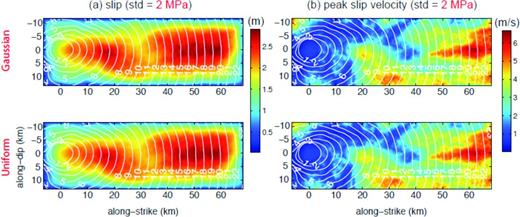
The distribution of kinematic source parameters obtained from spontaneous dynamic rupture modelling with the slip weakening friction law with different shapes of 1-point statistics, that is Gaussian and Uniform, but with the same standard deviation (=2 MPa). The rest of the format is the same as in Fig. 9. Although the input stress drop distributions have different shapes of 1-point statistics, both produce almost identical distributions of kinematic source parameters..
Auto (a) and crosscorrelation (b) structures for three kinematic source parameters in Fig. 12.
3.3 Near-source ground motions
The complexity of finite source processes can affect near-source ground motion characteristics significantly, especially for large events. It would be interesting to see how the differences we observe in the kinematic motions with the different standard deviations of input stress drop affect near-source ground motions. Fig. 14 shows the distribution of PGV (fault normal component) with three different standard deviations. The ratio of the PGVs from the models with the largest and lowest standard deviation (Fig. 14d) clearly shows three systematic distinctive patterns: (1) The increase of the standard deviation of stress drop increases the PGV in both the forward and backward directivity regions, being more pronounced near the end of the fault [e.g. station (c)]. It implies that large standard deviation (=3 MPa) increases the effect of forward rupture directivity. However, it also increases the PGV in the backward rupture directivity region although the absolute level of ground velocity is not as large as in the forward rupture directivity region. (2) The same effect is observed in the regions, surrounding the epicentre. This effect is also attributed to the rupture directivity from the hypocentre towards the free-surface. (3) On the contrary, it is interesting to see that in the regions perpendicular to the fault, outside the epicentre area, we observe the opposite effect, the PGVs actually decrease with the increase of standard deviation. These effects can also be observed in Fig. 15, where synthetic ground motions (fault normal comp) recorded at six different locations in Fig. 14(d) are displayed. Stations (a), (c) and (f) located respectively in the backward and forward directivity regions, and station (d) located around the epicentre area, show larger ground motions for the model with the largest standard deviation. The PGV increases almost by a factor of 2 at a certain location if the standard deviation increases to 3 MPa from 1 MPa. The large standard deviation also generates shorter waveform duration, indicating higher frequency content. At the stations (b) and (e) located in the region perpendicular to the fault, the differences of ground motion between models are opposite, that is, the stronger ground motion is attributed to the model with lower standard deviation. As expected in the kinematic source models, ground motions from two different PDFs (e.g. Gaussian and Uniform) are almost identical as shown at the bottom three panels in Fig. 15. This pattern is also observed when the standard deviation of input stress drop is 1 and 3 MPa as shown in Fig. S7. This may also indicate that the standard deviation is a more primary component in determining near-source ground motions rather than the detailed shape of PDF.
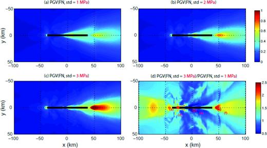
The distribution of peak ground velocity (PGV, fault normal component) with three different standard deviation values of input stress drop, (a) 1 MPa, (b) 2 MPa and (c) 3 MPa. The bottom right (d) panel shows the ratio of PGV (std = 3 MPa) to PGV (std = 1 MPa). PGV values increase significantly with standard deviation, especially in the forward and backward rupture directivity region. The solid black line and red star indicates the surface projection of the faulting plane and nucleation point, respectively. Red labels (a)–(f) denote the location of recorded waveforms shown in Fig. 15.
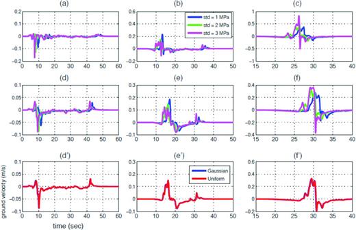
Waveforms (Fault normal) recorded at six different locations denoted in Fig. 15d. Note that PGV increases by a factor of 2 at a certain location as shown in panel (c). Bottom three panels (d’, e’, f’) show waveforms with std = 2 MPa, but for both Gaussian and Uniform distributions. As expected in kinematic motions, they show almost identical ground motions.
4 DISCUSSION
Mean stress drop is an important parameter in dynamic modelling because it affects the seismic moment of the event, generated by the dynamic modelling, and consequently ground motions as well. Andrews (1980) proposes the k−1 spectral decay rate of stress drop based on the theory of self-similarity for 2-point autocorrelation in stress field. However, the standard deviation of stress drop is not explicitly considered in most source modelling studies, consequently not well constrained yet. However, this study shows that the standard deviation of stress drop may affect resulting kinematic source motions and near-source ground motions significantly. The remaining question is how to constrain the 1-point statistics of stress drop, and dynamic input parameters in general. The heterogeneity of kinematic source parameters can be constrained by various types of geophysical data through kinematic source inversion, for example strong motion, teleseismic, GPS and InSAR, etc. Some attempts to constrain dynamic parameters (e.g. stress drop, strength excess, and slip weakening distance) with the kinematic source models from source inversion of past earthquakes have been reported (e.g. Ide & Takeo 1997; Tinti et al.2005). Although there may be a certain amount of uncertainty involved in the estimation process, because of the well-known limitations of kinematic source inversion models, these estimates may constrain 1-point statistics of dynamic parameters to the first degree. A robust constraint of dynamic parameters may also be achieved through the combination of detailed studies of lab experiment of friction, source inversion and full-scale simulations of ground-motion observations from many individual earthquakes based on a suite of earthquake dynamic model. This kind of study may constrain not only 1-point statistics of dynamic parameters, but also 2-point statistics, such as auto-correlation and crosscorrelations between dynamic parameters. Because current dynamic rupture simulations are physically consistent models, kinematic source quantities as well as ground motion metrics such as PGV, PGA and SAs can already benefit from them to evaluate 1-point and 2-point statistics of kinematic source and ground motion parameters.
It is encouraging that crosscorrelations between kinematic source parameters obtained by dynamic modelling (Fig. 11b) show consistent patterns with the findings by Song et al. (2009) and Song & Somerville (2010). We need to analyse a wide range of dynamic rupture models to have a general idea about the correlation structure between earthquake source parameters, but this analysis provides additional examples to support crosscorrelation with maximum values at non-zero offset distances. In addition, as demonstrated in Fig. 11(b), the standard deviation of input stress drop may be one key parameter that controls the correlation structure between kinematic source parameters. Once both 1-point and 2-point statistics of kinematic source parameters are constrained from dynamic rupture modelling (Figs 10 and 11), we can also simulate a large number of kinematic source models that reproduce the extracted source statistics by stochastic modelling (Song & Somerville 2010). These kinematic source models are supposed to contain physical self-consistency embedded in spontaneous dynamic rupture models in the sense that these models are constrained by 1-point and 2-point source statistics inferred from dynamic rupture modelling. This statement naturally indicates that 1-point and 2-point statistics of kinematic source parameters can be implemented in pseudo-dynamic source modelling (Guatteri et al.2004; Schmedes et al.2010; Song & Somerville 2010; Mena et al.2012).
6 CONCLUSIONS
This study demonstrates that at least two statistical measures, that is 1-point and 2-point statistics, are needed to quantify the heterogeneity of spatial data, and that 1-point statistics, especially the standard deviation of earthquake source parameters is an important element in characterizing the spatial distribution of source parameters because it may affect resulting kinematic source and ground motions significantly. Both 1-point and 2-point statistics of kinematic source parameters are significantly and systematically affected by the perturbation of input stress drop. The standard deviations also strongly control ground motions, especially in the rupture directivity region. These results underline the importance of 1-point statistics in earthquake source modelling and support the statement that we need to consider and constrain 1-point statistics of input source parameters more explicitly and carefully in earthquake source modelling. Finally, quantifying the characteristics of earthquake source and ground motions in the same format of 1-point and 2-point statistics may help us to study the effect of earthquake rupture processes on near-source ground motion characteristics within a consistent framework.
The authors thank E. Fukuyama (associate editor), A. Herrero, and one anonymous reviewer for thoughtful comments and suggestions for the original manuscript. The authors also thank A. Bizzarri, T. Uchide, J.-P. Ampuero and P.M. Mai for helpful discussion about this study. This study was funded by the NERA projects (Network of European Research Infrastructures for Earthquake Risk Assessment and Mitigation) from the 7th Framework Programme by the European Commission, the Swiss National Science Foundation (SNF), SNF Grant 200021–140459, and COGEAR project funded by the Competence Center for Environment and Sustainability of the ETH Domain (CCES). Simulations were done at the Swiss National Supercomputing Center (CSCS), under the production project ‘Development of Dynamic Rupture Models to Study the Physics of Earthquakes and Near-Source Ground Motion’.
REFERENCES
APPENDIX A: TRANSFORM OF 1-POINT STATISTICS
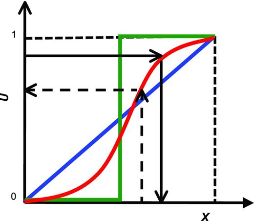
Schematic diagram that explains the transform of 1-point variability. If the red curve is a graphic representation of the cumulative density function, FX(x), for random variable, X, 1-point statistics can be transformed between a uniform distribution and a certain continuous distribution, FX(x), by following the path of black arrows. Both blue and dark green lines indicate two extreme cases where random variable, X, follows a uniform distribution or its probability density function (PDF) is a Dirac-delta function.
SUPPORTING INFORMATION
Additional Supporting Information may be found in the online version of this article:
Figure S1. Input stress drop distributions with the Gaussian (a) and Uniform (b) 1-point statistics. Both distributions have the same mean stress drop (=3 MPa), standard deviation (=1 MPa), and spectral decay rate (=k−1). Because of the small standard deviation (=1 MPa), the distribution with the Uniform distribution (bottom panel) has no negative stress drop.
Figure S2. Input stress drop distributions with the Gaussian (a) and Uniform (b) 1-point statistics. Both distributions have the same mean stress drop (=3 MPa), standard deviation (=3 MPa) and spectral decay rate (=k−1). Because of the large standard deviation (=3 MPa), even the distribution with the Uniform distribution (bottom panel) has a fair amount of negative stress drop.
Figure S3. The distribution of kinematic source parameters obtained from spontaneous dynamic rupture modelling with the slip weakening friction law with different shapes of 1-point statistics, that is Gaussian and Uniform, but with the same standard deviation (=1 MPa). The rest of the format is the same as in Fig. 12. As we see in Fig. 12, both distributions produce almost identical kinematic source parameters.
Figure S4. The distribution of kinematic source parameters obtained from spontaneous dynamic rupture modelling with the slip weakening friction law with different shapes of 1-point statistics, that is Gaussian and Uniform, but with the same standard deviation (=3 MPa). The rest of the format is the same as in Fig. 12. We observe small differences between two cases when the standard deviation is large (=3 MPa).
Figure S5. Auto (a) and crosscorrelation (b) structures for three kinematic source parameters in Fig. S3. The standard deviation of input stress drop is 1 MPa in this modelling. Both distributions (Gaussian and Uniform) produce almost identical auto- and crosscorrelation structures.
Figure S6. Auto (a) and crosscorrelation (b) structures for three kinematic source parameters in Fig. S4. The standard deviation of input stress drop is 3 MPa in this modelling. Both distributions (Gaussian and Uniform) produce almost identical auto- and crosscorrelation structures.
Figure S7. Waveforms (Fault normal component) recorded at three different locations denoted in Fig. 15d. Top three panels show waveforms with the standard deviation 1 MPa for both Gaussian and Uniform distributions. Bottom three panels show waveforms with the standard deviation 3 MPa. As expected in the distributions of kinematic source parameters (S3 and S4), two distributions (Gaussian and Uniform) show almost identical near-source ground motion waveforms at three selected sites with the standard deviation of input stress drop 1 and 3 MPa. (Supplementary Data)
Please note: OUP are not responsible for the content or functionality of any supporting materials supplied by the authors. Any queries (other than missing material) should be directed to the corresponding author for the article.
