


Abstract
Neurons in the inferior temporal (IT) cortex of monkeys respond selectively to complex visual stimuli, such as faces. Single neurons in the IT cortex encode different kinds of information about visual stimuli in their temporal firing patterns. To understand the temporal aspects of the information encoded at a population level in the IT cortex, we applied principal component analysis (PCA) to the responses of a population of neurons. The responses of each neuron were recorded while visual stimuli that consisted of geometric shapes and faces of humans and monkeys were presented. We found that global categorization, i.e. human faces versus monkey faces versus shapes, occurred in the earlier part of the population response, and that fine categorization occurred within each member of the global category in the later part of the population response. A cluster analysis, a mixture of Gaussians analysis, confirmed that the clusters in the earlier part of the responses represented the global category. Moreover, the clusters in the earlier part separated into sub-clusters corresponding to either human identity or monkey expression in the later part of the responses, and the global categorization was maintained even after the appearance of the sub-clusters. The results suggest that a hierarchical relationship of the test stimuli is represented temporally by the population response of IT neurons.
Introduction
A substantial number of neurons in the inferior temporal (IT) cortex respond to faces or complex objects (Bruce et al., 1981; Fujita et al., 1992). The responses of a population of neurons in the IT cortex encode individual faces based on their physical features (Hasselmo et al., 1989; Young and Yamane, 1992). Young and Yamane recorded single-unit activity during the presentation of 32 human-face images and calculated population activity vectors consisting of the mean firing rates of individual neurons for each stimulus. The population activity vectors were of high dimensions, and it was necessary to reduce the dimensions to visualize the behavior of the vectors. They applied multi-dimensional scaling (MDS), and found that the population activity vectors for facial stimuli with similar physical features were closely arranged in two-dimensional space. They calculated the population activity vectors from the mean firing rates and their temporal property remained unknown. Recently, it was reported that the responses of single neurons to complex visual stimuli convey different kinds of information along the time axis (Sugase et al., 1999; Tamura and Tanaka, 2001). For example, information about global categorization, i.e. human faces versus monkey faces versus shapes, was conveyed in the earliest part of the responses. Information about fine categorization within each member of the global category, i.e. either the identity or expression of faces, was represented later, beginning on average 51 ms after information about the global categorization was conveyed (Sugase et al., 1999). Therefore, the dynamics of neuronal responses in the IT cortex are important for representing visual information at different categorical levels at different times. Another study (Tamura and Tanaka, 2001) reported that the responses to visual stimuli became more selective later in the responses than in the initial transient part of the responses. In these reports, however, the authors were interested in the information encoded temporally by individual neurons and did not study the temporal aspects of information coding at the population level.
Here, to understand the temporal aspects of information coding at a population level in the IT cortex, we analyzed the population activity across a number of individually recorded neurons using principal component analysis (PCA) (Jollife, 1986), which is similar to MDS. Earlier observations of Sugase et al. (1999) suggested that global categorization occurs before fine categorization. In this study, we investigated how complex visual stimuli are represented along the time axis with respect to the responses of the neuronal population.
We addressed three points that remained unsolved in our previous study (Sugase et al., 1999). Previously, we described one type of neuron that encoded information about both global and fine categorizations in its responses. To examine information coding at a population level, the present study analyzed the responses of several types of neurons, including neurons that encoded both global and fine information, and also neurons that encoded only global information or only fine information. Second, to evaluate whether our a priori classification of the stimuli, i.e. global and fine categorization (Sugase et al., 1999), was appropriate, we used a cluster analysis, a mixture of Gaussians analysis. Using the cluster analysis, we were able to classify the population activity vectors for individual stimuli without an arbitrary categorization of the stimulus. We assessed our a priori classification by comparing the clusters produced in the cluster analysis. Third, we were especially interested in whether global categorization was retained after the occurrence of fine categorization within each member of the global category, i.e. whether the test stimuli were represented hierarchically along the time axis. Preliminary results have been presented in abstract form (Matsumoto et al., 2001).
Methods
Neuronal data were collected from two macaque monkeys (Macaca fuscata). All the details of the experimental procedures are described in Sugase et al. (1999). The procedures were approved by the Animal Care and Use Committee of the Neuroscience Research Institute/Electrotechnical Laboratory and were in accordance with the Guide for the Care and Use of Laboratory Animals as adopted by the NRI/ETL. In brief, single-unit activities of 1885 neurons were recorded in the IT cortex. The neuronal responses of each unit were studied while the monkey performed a fixation task. Thirty-eight visual stimuli were used in the task. The stimuli consisted of 16 monkey faces (four models with four expressions, i.e. neutral, pout-lipped, mid-open-mouthed and full open-mouthed faces), 12 human faces (three models with four expressions, i.e. neutral, happy, surprised and angry faces) and 10 geometric shapes (rectangles and circles, each in one of five colors, i.e. red, blue, green, pink and brown) as shown in figure 1 in Sugase et al. (1999). During the fixation task, the monkey started each trial by pressing a button. A fixation spot (a small red spot of 0.3°) appeared in the center of a color monitor screen that was located 48 cm in front of the eyes, and was displayed for 600 ms. The fixation spot was replaced by a blank gray background for 250 ms, and then one of the test stimuli was presented for 350 ms. An error was registered if the monkey moved its eyes beyond a fixation limit (within ±1° of the fixation spot). The neuronal activities were recorded with 1 ms time resolution. Of the 1885 neurons recorded, 169 neurons responded to at least one of the face stimuli [threshold criterion, the mean + 2SD of the responses within a 140 ms period before the stimulus onset (P < 0.05)]. Of the 169 neurons, we tested 97 using all stimuli from at least two of the three stimulus sets (i.e. two sets from the human face, monkey face or shape sets), and tested 45/97 neurons using all 38 test stimuli (i.e. all stimulus sets). To analyze how the responses of a population of IT neurons represented all test stimuli quantitatively, we used the data for the 45 neurons that we tested using all 38 test stimuli. Some of the neuronal data given here were taken from Sugase et al. (1999).
Principal Component Analysis
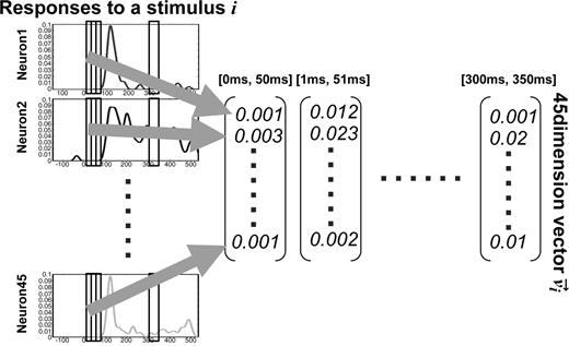
For the population analysis, we calculated a population activity vector for each stimulus. The procedure used to calculate the population activity vectors is summarized in Figure 1. A spike density function was obtained by averaging the spike counts between time t (ms) and t + 1 over the number of trials, and it was smoothed using a Gaussian filter with a variance of 10 ms. The population activity vector vi for test stimulus i consisted of the mean firing rates of 45 neurons that were recorded individually. The mean firing rates were obtained by averaging the spike density function within a 50 ms time window. Each population activity vector had 45 dimensions. Within the 50 ms time window, there were 38 population activity vectors for the 38 test stimuli. The start time of the time window was incremented by 1 ms from 0 ms (at the beginning of the presentation of the test stimuli) to 300 ms. This shift enabled observation of the temporal aspects of the neuronal population.
The procedure used to calculate the population activity vectors. The population activity vector vi for the visual stimulus i consists of the mean firing rates of 45 neurons within a 50 ms time window. The start time of the window is incremented by 1 ms from 0 ms (at the beginning of the presentation of the stimuli) to 300 ms.
Principal component analysis (PCA) is a dimension-reduction method that rearranges data in a high-dimensional space into a lower-dimensional space while preserving as much of the information in the high-dimensional data as possible. PCA was applied to the 38 population activity vectors in each time window. The greatest variance of the population responses was represented in the first principal component and the second greatest variance was represented in the second principal component.
Mixture of Gaussians Analysis
We used a mixture of Gaussians analysis to cluster the population activity vectors. We assumed that the 38 population activity vectors v = { v1, v2,…, v38} were generated from 45-dimensional Gaussian distributions, i.e. a mixture of Gaussians. Variational Bayes (VB) algorithm (Attias, 1999; Ghahramani and Beal, 2000) was used to estimate the parameters of the mixture of Gaussians, i.e. the means, variances, mixing ratios and number of the 45-dimensional Gaussian distributions. We estimated the number of Gaussians corresponding to the number of clusters from the free energy, which indicates the distance between the estimated mixture of Gaussians and the most appropriate mixture of Gaussians (Attias, 1999; Ghahramani and Beal, 2000). As the free energy increases, the estimated mixture of Gaussians approaches the most appropriate one (Attias, 1999; Ghahramani and Beal, 2000). We set the number of Gaussians from 1 to 10 and calculated the free energy 20 times for each number of Gaussians. Then, we examined the parameters and the number of Gaussians at which the free energy was the maximum. When the free energy is maximal, the members of each cluster are also determined. For example, let us assume that there are vectors and two clusters (A and B). The free energy is calculated for two cases: when one of the vectors belongs to cluster A and when the same vector belongs to cluster B. If the value of the free energy is larger when the vector belongs to cluster A than to cluster B, the vector is assigned as a member of cluster A. Similarly, the members of each cluster are determined.
Results
Results of PCA
We analyzed the responses of 45 neurons at the population level (see Methods). The responses of the 45 neurons were recorded individually. First, we classified the 45 neurons using the information-theoretic analysis that was used in Sugase et al. (1999). For the responses of each neuron, we calculated the information transmission rate for one global (human faces versus monkey faces versus shapes) category and six fine (human identity, human expression, monkey identity, monkey expression, shape color, and shape form) categories. We found that 36/45 neurons encoded both global and fine information, 7/45 neurons encoded only global information and the remaining 2/45 encoded only fine information.
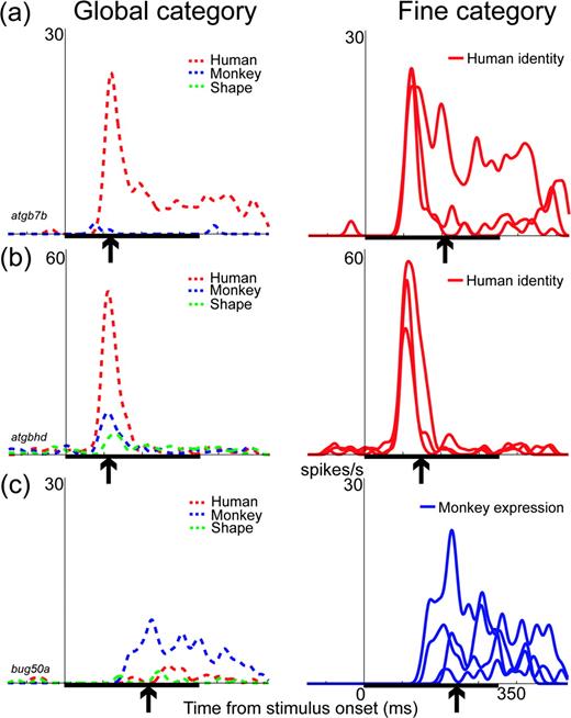
As we reported previously, information on the global category was transmitted before information on the fine category, with an average difference in latency of 51 ms, although there was substantial variation across the neurons (SD = 39 ms, n = 32; Sugase et al., 1999). The time of the peak information transmission rate for both the global and fine categories also varied cell-by-cell, and was 152 ± 57 ms (mean ± SD) for global information and 179 ± 49 ms for fine information. One reason for the variation among the neurons was that each neuron had a different temporal firing pattern. In the example shown in Figure 2a, some neurons had both initial transient and later sustained responses, whereas others showed only an initial transient response (Fig. 2b) or a later sustained response (Fig. 2c). The peak times for global information were 117, 109 and 213 ms after the stimulus onset for the neurons in Figure 2a,b,c, respectively (Fig. 2, arrows in the left panels). The peak times for fine information also varied among the neurons, and were 205, 149 and 245 for the respective neurons (Fig. 2, arrows in the right panels). The peak time for the global information preceded the peak time for the fine information. The intervals between these two peak times varied among the neurons, and were 88, 40 and 32 ms for the respective neurons.
Examples of the responses of three neurons that encoded both global and fine information. For each cell, the left panel shows the summed response for members of a global category, i.e. human faces (red dashed line), monkey faces (blue dashed line) and shape forms (green dashed line). The right panel shows the summed response for members of a fine category. For the neurons in (a) and (b), the responses are summed for three different human identities (red solid lines). For the neuron in (c), the responses are summed for four different monkey expressions (blue solid lines). All three neurons encode global information. For fine information, the neurons in (a) and (b) encode information about human identity, and the neuron in (c) encodes information about monkey expression. The arrow under the abscissa in each plot shows the time of the peak information transmission rate for each category. The thick black bar on the abscissa indicates the 350 ms period of stimulus presentation.
Having the cell-by-cell variation for the intervals between the peak times of these two information measures, we decided to perform a population analysis to see how the IT neurons represented the test stimuli along the time axis. For the population analysis, we calculated 38 population activity vectors consisting of the mean firing rates of the 45 neurons for the 38 test stimuli within a 50 ms time window, moving in 1 ms steps. We applied PCA to the 38 population activity vectors in each time window. Consequently, the 38 population activity vectors in the 45-dimensional space projected onto 38 vectors in the two-dimensional space. To determine the time windows in which global or fine categorization occurred, we calculated the distances between the population activity vectors. The center coordinates for vectors that belonged to either global or fine categories were determined by averaging the coordinates for the vectors. For the global category, three distances were measured, i.e. the distance between the center of the human face vectors and the center of the monkey face vectors, the distance between the center of the monkey face vectors and the center of the shape vectors, and the distance between the center of the human face vectors and the center of the shape vectors. The sum of the three distances was the maximum in the [90 ms, 140 ms] time window. For the fine category, the distances between the centers of the vectors were measured and summed within each member of the global category, i.e. human identity, monkey expression and shape form. The sum of the distances for human identity, monkey expression, and shape form was the maximum in the [140 ms, 190 ms] window. Therefore, the [90 ms, 140 ms] window was regarded as the time window when global categorization occurred, and the [140 ms, 190 ms] window was regarded as the time window for fine categorization.
To examine whether only a few neurons determine the distribution of the population activity vectors, we calculated the eigenvectors that determined both the first and second principal components. The first principal component was determined by the eigenvector shown in Figure 3a. The second principal component was determined by the eigenvector shown in Figure 3b. A neuron with a higher value of the element contributes more to setting a principal component. From Figure 3a,b, it is clear that the distribution of the values is not biased toward a small number of neurons, indicating that more than a small number of neurons contribute to setting both the first and second principal components. We also checked the eigenvalues to see how each principal component contributed to the PCA space (Fig. 3c). The eigenvalue indicates how much of the variance in the data is represented along each axis. The eigenvalue of the first principal component was largest, indicating that the first principal component represented most of the variance in the population response.
![Eigenvectors and eigenvalues for the PCA analysis. (a) The eigenvector of the first principal component for the [90 ms, 140 ms] and [140 ms, 190 ms] time windows. (b) The eigenvector of the second principal component for the [90 ms, 140 ms] and [140 ms, 190 ms] windows. The horizontal axis indicates neurons (from 1 to 45), while the vertical axis indicates the value of each element that constitutes the eigenvector. (c) The eigenvalues for the [90 ms, 140 ms] and [140 ms, 190 ms] windows. The horizontal axis indicates the dimension (from 1 to 45), while the vertical axis indicates the eigenvalues. For the [90ms, 140ms] window, eigenvalues of first, second and third principal components are 0.0038 (contribution ratio: 53.4%), 0.0010 (14.3%) and 0.0008 (11.7%), respectively. For the [140ms, 190ms] window, eigenvalues of first, second and third principal components are 0.0056 (55.2%), 0.0012 (11.9%) and 0.0008 (8.5%), respectively.](https://oup.silverchair-cdn.com/oup/backfile/Content_public/Journal/cercor/15/8/10.1093/cercor/bhh209/2/m_cercorbhh209f03_lw.jpeg?Expires=1716875235&Signature=YYDDH4rW~yZ~YhSpXe7kaO-U1V02P3c8YsbitTAfiqWeP9jTZWhz3B5MpvQBwpxnc5XXDXOq3P96TpCjmamf2Vu~tAZ5DYhgf2Tzgz6VSIPcSbvNbsBXVZ-jB8zrpv2LUyNF0ij~zHYjNLFBTjC6UeVneTxag7Y0~U5GH34ARuGyIP7A9NkcbObZC4wmiBeqa8o3gZNQVmHct4rXVG98PlR2Qlon83mIRl-NzpDDa42t8RClmOVrg6PDO2~SWoIwCvnqJMSr09a3LHwxC~Umt07GipL9E0mluuEjcIEFL7tsc3GVfl-OlQeB1gEUbTuceqmuAZlxJkASrlc8FtbbGw__&Key-Pair-Id=APKAIE5G5CRDK6RD3PGA)
Eigenvectors and eigenvalues for the PCA analysis. (a) The eigenvector of the first principal component for the [90 ms, 140 ms] and [140 ms, 190 ms] time windows. (b) The eigenvector of the second principal component for the [90 ms, 140 ms] and [140 ms, 190 ms] windows. The horizontal axis indicates neurons (from 1 to 45), while the vertical axis indicates the value of each element that constitutes the eigenvector. (c) The eigenvalues for the [90 ms, 140 ms] and [140 ms, 190 ms] windows. The horizontal axis indicates the dimension (from 1 to 45), while the vertical axis indicates the eigenvalues. For the [90ms, 140ms] window, eigenvalues of first, second and third principal components are 0.0038 (contribution ratio: 53.4%), 0.0010 (14.3%) and 0.0008 (11.7%), respectively. For the [140ms, 190ms] window, eigenvalues of first, second and third principal components are 0.0056 (55.2%), 0.0012 (11.9%) and 0.0008 (8.5%), respectively.
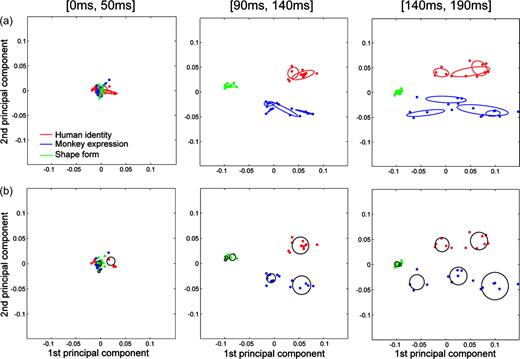
Figure 4 shows the distributions of the 38 population activity vectors in the two-dimensional space in the [90 ms, 140 ms] and [140 ms, 190 ms] time windows together with the [0 ms, 50 ms] window, which was the initial condition of the population vectors. The contribution ratio was 34.2% in the [0 ms, 50 ms] time window, 67.7% in the [90 ms, 140 ms] window and 67.1% in the [140 ms, 190 ms] window. The ratios in the [90 ms, 140 ms] and [140 ms, 190 ms] time windows were high, given the reduction from 45 dimensions to only two dimensions, suggesting that the information encoded in the [90 ms, 140 ms] and [140 ms, 190 ms] windows in the two-dimensional space preserved the information in the 45-dimensional space well. In the [0 ms, 50 ms] time window, all the distributions overlapped. In the [90 ms, 140 ms] window, the distribution pattern suggested that global categorization, i.e. human faces versus monkey faces versus shapes, occurred during this time period (Fig. 4a). In the [140 ms, 190 ms] window, the distances between the distributions of each member of the global category were maintained (Fig. 4a). In addition, the human identity distributions (Fig. 4b) and the monkey expression distributions (Fig. 4c) were separated. But, the human expression distribution (Fig. 4c) and monkey identity distribution (Fig. 4b) still overlapped. The distribution pattern suggested that fine categorization, i.e. human identity or monkey expression, occurs during the [140 ms, 190 ms] window, while global categorization was maintained. These results suggest that the hierarchical relationship of the test stimuli is represented by the dynamics of neuronal responses at the population level.
![Population activity vectors in two-dimensional space rearranged using PCA in the [0 ms, 50 ms], [90 ms, 140 ms] and [140 ms, 190 ms] windows. The horizontal axis represents the first principal component, while the vertical axis represents the second principal component. The points indicate the population activity vectors for the individual stimuli. The colors of the points represent the global category: the vectors for human faces, monkey faces and shapes are shown in red, blue and green, respectively. The ellipses indicate the distributions of the population activity vectors for the global (a) and fine (b and c) categories. (a) The distributions for human faces, monkey faces, and shape are shown as red, blue and green ellipses, respectively (dashed line). (b) The distributions for human identity, monkey identity, and shape form are shown as red, blue and green ellipses, respectively (solid line). (c) The distributions for human expression, monkey expression and shape color are shown as red, blue and green ellipses, respectively (solid line). The ellipses were drawn by calculating the averages and co-variances of the coordinates of the points. The center of each ellipse is plotted so that it is located at the average point. The direction of the ellipse and the length of the major and minor axes were calculated from the covariance.](https://oup.silverchair-cdn.com/oup/backfile/Content_public/Journal/cercor/15/8/10.1093/cercor/bhh209/2/m_cercorbhh209f04_4c.jpeg?Expires=1716875235&Signature=RG0SgbihxLTku0GoeWq4efkhWLDaSfGAsZR3s05O5EsbMj2YnXNTqXFoETPsBPUR79sgDlpztWdluC1pAK9weNztfY4DcG4X-ssoE4s~ixFiY7WAQVaKgHPOZ-7RpqVhRmjqiLkQFTp~EBCmXkHNELKCBnY9V1HykxtEl3JjyGG-B8QPk-NbiwQjbBPdpR7HjomsIMWDxThpp6PelaklzJFwhUHk-QrH9aNwKR6NBIe-cHfwp5~QzSBukjjdNY4FfJ604SYNAJ6j14GkLd4oMRSkjk95VQe2Qx2WCQIQERqBXgJQ2tdXJyEfsHVmzIFmRb6uy23IaE5ZgkoyWXxK9Q__&Key-Pair-Id=APKAIE5G5CRDK6RD3PGA)
Population activity vectors in two-dimensional space rearranged using PCA in the [0 ms, 50 ms], [90 ms, 140 ms] and [140 ms, 190 ms] windows. The horizontal axis represents the first principal component, while the vertical axis represents the second principal component. The points indicate the population activity vectors for the individual stimuli. The colors of the points represent the global category: the vectors for human faces, monkey faces and shapes are shown in red, blue and green, respectively. The ellipses indicate the distributions of the population activity vectors for the global (a) and fine (b and c) categories. (a) The distributions for human faces, monkey faces, and shape are shown as red, blue and green ellipses, respectively (dashed line). (b) The distributions for human identity, monkey identity, and shape form are shown as red, blue and green ellipses, respectively (solid line). (c) The distributions for human expression, monkey expression and shape color are shown as red, blue and green ellipses, respectively (solid line). The ellipses were drawn by calculating the averages and co-variances of the coordinates of the points. The center of each ellipse is plotted so that it is located at the average point. The direction of the ellipse and the length of the major and minor axes were calculated from the covariance.
Results from the Mixture of Gaussians Analysis
PCA separated the distributions of human, monkey, and shape in the [90 ms, 140 ms] time window. Therefore, global categorization, i.e. human versus monkey versus shape, occurred during this period. In the [140 ms, 190 ms] window, the individual distributions of human identity and monkey expression were separated. Therefore, fine categorization, i.e. human identity or monkey expression, occurred during this period. We re-plotted the PCA space in which the ellipses now represent the distributions of human identity, monkey expression, or shape form in Figure 5a. To investigate whether both the global and fine categorizations approximated what the neuronal responses represented, we applied a cluster analysis, a mixture of Gaussians analysis, to the 45-dimensional population activity vectors in each time window (see Methods).
Comparison of the distributions of the population activity vectors for the fine categories and the distributions in the cluster analysis. These figures are the same as Figure 4, except what the ellipses indicate. (a) The red, blue and green ellipses indicate the distributions of the population activity vectors for the fine categories human identity, monkey expression and shape-form, respectively. (b) The clusters obtained from the mixture of Gaussians analysis are shown as circles. The center of each circle is plotted so that it is located at the average value of the coordinates of the points. The radius of the circle was calculated from the standard deviation of the coordinates of the points.
The clusters obtained using the mixture of Gaussians analysis in the [0 ms, 50 ms], [90 ms, 140 ms], and [140 ms, 190 ms] windows are shown as circles in Figure 5b. There were 3, 6 and 7 clusters in the [0 ms, 50 ms], [90 ms, 140 ms] and [140 ms, 190 ms] windows, respectively. The members of each cluster in the [90 ms, 140 ms] and [140 ms, 190 ms] windows are shown in Figure 6a,b. The [90 ms, 140 ms] window contained clusters corresponding to human faces, monkey faces and shapes (Fig. 6a). In addition, six monkey faces with a open mouth were separated from the other monkey faces. In the [140 ms, 190 ms] window, some clusters that were found in the [90 ms, 140 ms] window were separated into sub-clusters (Fig. 6b). The human face cluster in the [90 ms, 140 ms] window was separated into two sub-clusters. The two monkey face clusters in the [90 ms, 140 ms] window were separated into three sub-clusters (Fig. 6b).
![Members of individual clusters obtained through the mixture of Gaussians analysis. The results in the (a) [90 ms, 140 ms] and (b) [140 ms, 190 ms] windows. The ellipses indicate the clusters corresponding to the circles in Figure 5b. Each image shows a test stimulus of each population activity vector. For monkey faces, the [90 ms, 140 ms] window (a) contains two clusters: one (on the right) contains all four full open-mouthed and two mid-open-mouthed faces. In the full open-mouthed faces, the monkeys have their mouths wide open, showing their teeth. The other cluster (on the left) contains the remaining faces, i.e. all four neutral, four pout-lipped and two mid-open-mouthed faces. In the [140 ms, 190 ms] window (b), the right monkey cluster in (a) is maintained and the left monkey cluster is further separated into two sub-clusters: one (on the left) containing three pout-lipped and one neutral face, and the other (in the middle) containing three neutral faces, two mid-open-mouthed faces and one pout-lipped face.](https://oup.silverchair-cdn.com/oup/backfile/Content_public/Journal/cercor/15/8/10.1093/cercor/bhh209/2/m_cercorbhh209f06_4c.jpeg?Expires=1716875235&Signature=EPxSJqtu5cJOfBXJX~dYEjS5yA4i~FygcGx7xxLmEjBeS7d~OWrbqJWs6C91hkwehUFg5VmF3cuIfUmrSwzs-zbK-I3RymbY5~QHOyUtLSuAM9wxv4RhPgB3IKjmJ~c9vgbi~rjRjD81FU~AxzClf9LxvwHzsEhjz8jhgzY6LL6q~F-XTxLz6vsclEf-ymA3jjtmkTrLZ1fHPBo8NonboJnTsc9Dv4GXqmFXi8QALwEz-8uG5IPMc9p~~nfOx0QjYi3FgP2XMjMOPpwMGddSFJvAhiGVMUF-n1dSfLImQ3cnlHYLNI~MHtUpT-gG3C8yH~mlXJbd4jvPqJDPJUm5bg__&Key-Pair-Id=APKAIE5G5CRDK6RD3PGA)
Members of individual clusters obtained through the mixture of Gaussians analysis. The results in the (a) [90 ms, 140 ms] and (b) [140 ms, 190 ms] windows. The ellipses indicate the clusters corresponding to the circles in Figure 5b. Each image shows a test stimulus of each population activity vector. For monkey faces, the [90 ms, 140 ms] window (a) contains two clusters: one (on the right) contains all four full open-mouthed and two mid-open-mouthed faces. In the full open-mouthed faces, the monkeys have their mouths wide open, showing their teeth. The other cluster (on the left) contains the remaining faces, i.e. all four neutral, four pout-lipped and two mid-open-mouthed faces. In the [140 ms, 190 ms] window (b), the right monkey cluster in (a) is maintained and the left monkey cluster is further separated into two sub-clusters: one (on the left) containing three pout-lipped and one neutral face, and the other (in the middle) containing three neutral faces, two mid-open-mouthed faces and one pout-lipped face.
Mutual information (bits) between each category and clusters obtained by the mixture of Gaussians analysis
| [90 ms, 140 ms] | [140 ms, 190 ms] | |
|---|---|---|
| Global | 1.56 | 1.56 |
| Fine: human identity | 0 | 0.71 |
| Fine: human expression | 0 | 0.06 |
| Fine: monkey identity | 0.05 | 0.1 |
| Fine: monkey expression | 0.71 | 0.91 |
| Fine: shape form | 1 | 1 |
| Fine: shape color | 0.36 | 0 |
| [90 ms, 140 ms] | [140 ms, 190 ms] | |
|---|---|---|
| Global | 1.56 | 1.56 |
| Fine: human identity | 0 | 0.71 |
| Fine: human expression | 0 | 0.06 |
| Fine: monkey identity | 0.05 | 0.1 |
| Fine: monkey expression | 0.71 | 0.91 |
| Fine: shape form | 1 | 1 |
| Fine: shape color | 0.36 | 0 |
The global category was human faces versus monkey faces versus shapes. The mutual information between each cluster and the global category approached its maximum value in the [90 ms, 140 ms] time window, and remained the same in the [140 ms, 190 ms] window. This suggests that the global category was represented in the [90 ms, 140 ms] time window and was maintained until the [140 ms, 190 ms] window. Regarding the information common to each cluster and the fine categories, the mutual information concerning both human identity and monkey expression was maximal in the [140 ms, 190 ms] time window, suggesting that this window represented the fine categories. There was little mutual information for both human expression and monkey identity. Therefore, when fine categorization occurred, human faces were classified mainly according to identity, and monkey faces were classified mainly according to expression. Mutual information between each cluster and the shape-form category was maximal in both the [90 ms, 140 ms] and [140 ms, 190 ms] windows, suggesting that the categorization of shapes according to their form occurred before the fine categorization of faces. Therefore, categorization occurred from the global category to the fine categories along the time axis, in which the fine categories corresponded to human identity and monkey expression. This implies that the population response of IT neurons represented a hierarchical relationship of the test stimuli temporally.
Discussion
To understand the temporal aspects of information encoding at the population level in the IT cortex, we analyzed the population response across 45 individually recorded neurons using PCA and a mixture of Gaussians analysis. Analysis of the individual neurons has showed that the information on global categorization increased ∼51 ms before the information on fine categorization (Sugase et al., 1999). The results of PCA indicated that global categorization occurred in the [90 ms, 140 ms] window and that fine categorization occurred in the [140 ms, 190 ms] window. In other words, the global categorization occurred ∼50 ms before the fine categorization.
Using the mixture of Gaussians analysis, we investigated whether both the global and fine categorizations were close approximations of what the neuronal responses represented. The [90 ms, 140 ms] window contained clusters corresponding to global categorization, i.e. human faces versus monkey faces versus shapes. In the [140 ms, 190 ms] window, human faces and monkey faces were separated into sub-clusters corresponding to either the human identity or monkey expression. We also found that the global categorization was maintained even after the sub-clusters appeared. Therefore, a hierarchical relationship of the test stimuli was represented.
For fine categorization, we found that human faces were classified mainly according to identity, rather than to expression, whereas monkey faces were classified mainly by expression. The monkey subjects might have difficulty in discriminating between either different human expressions or different monkey models using our test stimuli. It would be interesting to see behavioral data for monkeys that perform a discrimination task, such as the face identification task used by Eifuku et al. (2004), using the same test stimuli, to see whether the monkeys have difficulty in discriminating these two things.
How many faces can be represented in the monkey temporal cortex using this type of coding? For example, in this study, a population of 45 neurons encoded 0.71 bits for human identity. To represent as many as 100 human identities (6.6 bits) might need a population of neurons about nine times larger, i.e. ∼400 neurons, assuming that each population encodes information about human identity independently. As there are more than 400 neurons in the IT cortex, we believe that the IT neurons have the capacity to represent a much larger number of faces, using hierarchical coding.
We also found that in the [140 ms, 190 ms] window, fine categorization occurred within each member of the global category, while global categorization was maintained. This implies that the population of neurons extracts a hierarchical relationship from among the test stimuli and represents each stage of the hierarchy at a different time. This temporal hierarchical encoding might be useful for memory in the IT cortex. As the number of neurons in the IT cortex is limited, the neurons have to store information efficiently. Storing the information hierarchically along the time axis is one way of ensuring such efficient encoding. For example, when a human face is stored, it would be classified into a human group. The neurons that represent information regarding the human group would have to store only the differences between this face and other people's faces; they do not have to store all the possible relationships between this face and a wide variety of objects throughout the world. This reduces the effort needed to remember a face. Hierarchical encoding might have another benefit. As the amount of information stored in the IT cortex increases, more time is needed to search for a target. If the information is stored hierarchically, less time is needed to search for an object because global information can be used as a tag. For example, when we recognize a person by looking at his/her face, initially there is a search for the human faces category and then there is a search for the face among the human faces in memory. This would take less time than searching for the face directly among the large number of information items that humans habitually store. Therefore, hierarchical encoding would also be important because it enables a rapid search.
The next question is how the dynamics of information representation in the IT cortex are produced. The visual areas earlier than the IT cortex are thought to play a role in processing the more detailed features of a visual stimulus, so global and fine categorization of the test stimuli might not take place in these areas, whereas the global and fine relationship might be detected in the IT cortex. There are several neural network models that can reproduce our IT neuronal responses. As an example, Matsumoto and Okada (2004) examined whether a neural network within the IT cortex served an important role in forming the dynamics of the neurons. They used an attractor network (Amit, 1989), and found that the dynamics of their attractor network were qualitatively similar to the responses of the IT neurons recorded by Sugase et al. (1999). Another attractor model has been proposed for the hierarchical classification of odors (Ambros-Ingerson et al., 1990). This model includes feed-forward and feedback connections between two different areas (olfactory bulb and olfactory cortex), and might be applicable to our hierarchical processing of visual stimuli. Some neurons in the IT cortex have prolonged sustained activity that continues after the disappearance of a visual stimulus (Miyashita, 1988; Miyashita and Chang, 1988). Experimental evidence has shown that this type of mnemonic signal is triggered by a top-down signal from the prefrontal cortex (Tomita et al., 1999). Interactions between the IT cortex and prefrontal cortex might also be important in hierarchical representation. Yet another model is a feedforward model that includes both slow and fast pathways, in which global information is processed on a fast pathway and fine information is processed on a slow pathway. Therefore, either an intra- or inter-areal contribution might be important for the hierarchical representation of visual stimuli, or a hierarchical representation might already be observed in the visual cortex that sends its major output to the IT cortex. Interesting further studies into the neural mechanisms underlying the hierarchical representation might involve experimental manipulations such as the disruption of neuronal processing either within the IT cortex or between the IT cortex and other areas, or recording from the cortex that participates in an earlier processing stage along the ventral visual stream.
We thank Dr M. Kawato, Dr K. Doya and Dr F.A. Miles for their many valuable comments. We also thank Dr. M. Sato for discussion regarding the variational Bayes algorithm. This work was partially supported by Grant-in-Aid Scientific Research on Priority Areas No. 14084212 and Grant-in-Aid Scientific Research (C) No. 16500093, and it was performed as part of the Advanced and Innovational Research Program in Life Sciences of the Ministry of Education, Culture, Sports, Science and Technology, Japan.
References
Ambros-Ingerson J, Granger R, Lynch G (
Attias H (
Bruce C, Desimone R, Gross, CG (
Eifuku S, De Souza WC, Tamura R, Nishijo H, Ono T (
Fujita I, Tanaka K, Ito M, Cheng K (
Ghahramani Z, Beal MJ (
Hasselmo ME, Rolls ET, Baylis GC (
Matsumoto N, Okada M, Doya K, Sugase Y, Yamane S (
Matsumoto N, Okada M (
Miyashita Y (
Miyashita Y, Chang HS (
Sugase Y, Yamane S, Ueno S, Kawano K (
Tamura H, Tanaka K (
Tomita H, Ohbayashi M, Nakahara K, Hasegawa I, Miyashita Y (
Author notes
1PRESTO, Japan Science and Technology Agency, Saitama 351-0198, Japan, 2RIKEN Brain Science Institute, Saitama 351-0198, Japan, 3National Institute of Advanced Industrial Science and Technology (AIST), Ibaraki 305-8568, Japan, 4Kawato Dynamic Brain Project, ERATO, JST, Kyoto 619-0288, Japan, 5Graduate School of Frontier Sciences, University of Tokyo, Chiba 277-8561, Japan and 6Graduate School of Medicine, Kyoto University, Kyoto 606-8501, Japan