


Abstract
Motivation: With protein sequences entering into databanks at an explosive pace, the early determination of the family or subfamily class for a newly found enzyme molecule becomes important because this is directly related to the detailed information about which specific target it acts on, as well as to its catalytic process and biological function. Unfortunately, it is both time-consuming and costly to do so by experiments alone. In a previous study, the covariant-discriminant algorithm was introduced to identify the 16 subfamily classes of oxidoreductases. Although the results were quite encouraging, the entire prediction process was based on the amino acid composition alone without including any sequence-order information. Therefore, it is worthy of further investigation.
Results: To incorporate the sequence-order effects into the predictor, the ‘amphiphilic pseudo amino acid composition’ is introduced to represent the statistical sample of a protein. The novel representation contains 20 + 2λ discrete numbers: the first 20 numbers are the components of the conventional amino acid composition; the next 2λ numbers are a set of correlation factors that reflect different hydrophobicity and hydrophilicity distribution patterns along a protein chain. Based on such a concept and formulation scheme, a new predictor is developed. It is shown by the self-consistency test, jackknife test and independent dataset tests that the success rates obtained by the new predictor are all significantly higher than those by the previous predictors. The significant enhancement in success rates also implies that the distribution of hydrophobicity and hydrophilicity of the amino acid residues along a protein chain plays a very important role to its structure and function.
Contact: kchou@san.rr.com
1 INTRODUCTION
According to their EC (Enzyme Commission) numbers, enzymes are mainly classified into six families (Webb, 1992): (1) oxidoreductases, catalyzing oxidoreduction reactions; (2) transferases, transferring a group from one compound to another; (3) hydrolases, catalyzing the hydrolysis of various bonds; (4) lyases, cleaving C–C, C–O, C–N and other bonds by means other than hydrolysis or oxidation; (5) isomerases, catalyzing geometrical or structural changes within one molecule; and (6) ligases, catalyzing the joining together of two molecules coupled with the hydrolysis of a pyrophosphate bond in ATP or a similar triphosphate. Each of these families has its own subfamilies, and sub-subfamilies. For a newly found protein sequence, we are often challenged by the following two questions: is the new protein an enzyme or non-enzyme? If it is, to which enzyme family class should it be attributed? Both questions are very basic and essential because they are intimately related to the function of the protein as well as its specificity and molecular mechanism. Although the answers can be found through various biochemical experiments, it is both time-consuming and costly to completely rely on experiments. Particularly, the number of newly found protein sequences is now increasing rapidly. For instance, the number of total sequence entries in SWISS-PROT (Bairoch and Apweiler, 2000) was only 3939 in 1986; recently, it was expanded to 153 325 (increasing by more than 38 times in less than two decades!) according to Release 43.6 (June 21 2004) of SWISS-PROT (http://www.expasy.org/sprot/relotes/relstat.html). With such a sequence explosion, it has become vitally important to develop an automated and fast method to help deal with the above two fundamental problems. Actually, efforts have been made in this regard, and the results in identifying the attribute among the six main enzyme family classes as well as between enzymes and non-enzymes are quite promising (Chou and Cai, 2004). Since each of the main enzyme families has its own subfamilies, the next question is: for an enzyme with a given main family class, can we predict which subfamily it belongs to? This is indispensable if we wish to understand the molecular mechanism of the enzyme at a deeper level. In a previous study (Chou and Elrod, 2003), the covariant-discriminant predictor was adopted to identify the 16 subfamilies of oxidoreductases. However, in that study the entire approach was based on the protein amino acid composition alone. According to the classical definition, the amino acid composition of a protein consists of 20 components representing the occurrence frequencies of the 20 native amino acids in it. Obviously, if a protein sample is represented by its amino acid composition alone, all the details about its sequence order and sequence length are totally lost. Therefore, although the results obtained in that study (Chou and Elrod, 2003) are quite encouraging, the methodology is very preliminary and certainly worthy of further improvement. To include all the details of its sequence order and length, the sample of a protein must be represented by its entire sequence. Unfortunately, it is unfeasible to establish a predictor with such a requirement, as exemplified below. As mentioned above, the total number of sequence entries that contain 56 402 618 amino acids is 153 325 according to Release 43.6 of SWISS-PROT. And hence the average protein length is ∼368. The number of different combinations for a protein of 368 residues will be 20368 = 10368 log 20 > 10478! For such an astronomical number, it is impracticable, to construct a reasonable training dataset that can be used for a meaningful statistical prediction based on the current protein data. Besides, protein sequence lengths vary widely, which poses an additional difficulty for including the sequence-order information, in both the dataset construction and algorithm formulation. Faced with such a dilemma, can we find a compromise to partially incorporate the sequence-order effects? This problem is addressed in the next section.
2 THE AMPHIPHILIC PSEUDO AMINO ACID COMPOSITION
The sample of a protein can be represented by two different forms: one is the discrete form and the other is the sequential form. In the discrete form, a protein is represented by a set of discrete numbers or a multiple dimension vector. For example, the amino acid composition is a typical discrete form that has been widely used in predicting protein structural class (Bahar et al., 1997; Cai et al., 2000; Chandonia and Karplus, 1995; Chou and Zhang, 1993; Chou and Maggiora, 1998; Chou and Zhang, 1994; Chou, 1989; Deleage and Roux, 1987; Klein, 1986; Klein and Delisi, 1986; Kneller et al., 1990; Metfessel et al., 1993; Nakashima et al., 1986; Zhou, 1998; Zhou and Assa-Munt, 2001) and subcellular localization (Cedano et al., 1997, Chou, 2000, Chou and Elrod, 1999, Hua and Sun, 2001, Nakai, 2000, Nakai and Kanehisa, 1991, Nakashima and Nishikawa, 1994, Zhou and Doctor, 2003). The advantage of the discrete form is that it is easy to be treated in statistical prediction, but the disadvantage is, it is hard to directly incorporate the sequence-order information (the amino acid composition actually contains no sequence-order information at all, as mentioned in the last section). In the sequential form, a protein is represented by a series of amino acids according to the order of their positions in the protein chain. Therefore, the sequential form can naturally reflect all the information about the sequence order and length of a protein. However, when used in statistical treatment, it leads to the difficulty in dealing with an almost infinitive number of possible patterns, as illustrated above.
To solve such a dilemma, the crux is: can we develop a different discrete form to represent a protein that will allow accommodation of partial, if not all, sequence-order information? Since a protein sequence is usually represented by a series of amino acid codes, what kind of numerical values should be assigned to these codes in order to optimally convert the sequence-order information into a series of numbers for the discrete form representation? Here, we introduce the amphiphilic pseudo amino acid composition to tackle these problems.
Suppose a protein P with a sequence of L amino acid residues:
where R1represents the residue at chain position 1, R2 the residue at position 2, and so forth. Because the hydrophobicity and hydrophilicity of the constituent amino acids in a protein play a very important role in its folding, its interaction with the environment and other molecules, as well as its catalytic mechanism, these two indices may be used to effectively reflect the sequence-order effects. For example, many helices in proteins are amphiphilic, that is, formed by the hydrophobic and hydrophilic amino acids according to a special order along the helix chain, as illustrated by the ‘wenxiang’ diagram (Chou et al., 1997). Actually, different types of proteins have different amphiphilic features, corresponding to different hydrophobic and hydrophilic order patterns. In view of this, the sequence-order information can be indirectly and partially, but quite effectively, reflected through the following equations (Fig. 1):
where
where h1(Ri) and h2(Ri) are, respectively, the hydrophobicity and hydrophilicity values for the ith (i = 1,2,…,L) amino acid in Equation (1), and the dot (·) means the multiplication sign. In Equation (2), τ1 and τ2 are called the first-tier correlation factors that reflect the sequence-order correlations between all the most contiguous residues along a protein chain through hydrophobicity and hydrophilicity, respectively (Fig. 1, a1 and a2); τ3 and τ4 are the corresponding second-tier correlation factors that reflect the sequence-order correlation between all the second-most contiguous residues (Fig. 1, b1 and b2); and so forth. Note that before substituting the values of hydrophobicity and hydrophilicity into Equation (3), they were all subjected to a standard conversion as described by the following equation:
where we use the ℝi (i = 1,2,…,20) to represent the 20 native amino acids according to the alphabetical order of their single-letter codes: A, C, D, E, F, G, H, I, K, L, M, N, P, Q, R, S, T, V, W and Y. The symbols
where
where fi (i = 1,2,…,20) are the normalized occurrence frequencies of the 20 native amino acids in the protein P, τj the j-tier sequence-correlation factor computed according to Equation (2), and w the weight factor. In the current study, we chose w = 0.5 to make the results of Equation (6) within the range easier to be handled (w can be of course assigned with other values, but this would not make a significant difference to the final results). Therefore, the first 20 numbers in Equation (5) represent the classic amino acid composition, and the next 2λ discrete numbers reflect the amphiphilic sequence correlation along a protein chain. Such a protein representation is called ‘amphiphilic pseudo amino acid composition’, or abbreviated as Am-Pse-AA composition: it has the same form as the amino acid composition, but contains much more information that is related to the sequence order of a protein and the distribution of the hydrophobic and hydrophilic amino acids along its chain. It should be pointed out that, according to the definition of the classical amino acid composition, all its components must be ≥0; it is not always true, however, for the pseudo amino acid composition (Chou, 2001): the components corresponding to the sequence correlation factors may also be <0, as further discussed later.
3 AUGMENTED COVARIANT-DISCRIMINANT PREDICTOR
Since the Am-Pse-AA composition Equation (5) has the same mathematical frame as the amino acid composition except that it contains more components, all the existing predictors developed based on the classical amino acid composition can be straightforwardly extended to cover the Am-Pse-AA composition. For the reader's convenience, a brief description of how to augment the covariant-discriminant predictor for the Am-Pse-AA composition is given below. The details about the algorithm and its development can be found in a series of earlier papers (Chou and Zhang, 1995; Chou, 2001; Chou and Elrod, 1999; Chou and Zhang, 1994; Liu and Chou, 1998; Zhou, 1998; Zhou and Doctor, 2003). According to the Am-Pse-AA composition [Equation (5)], the k-th enzyme in the class m can be represented by a (20 + 2λ) D (dimension) vector as follows:
where
where
Suppose P is a query enzyme whose subfamily is to be identified. It is also represented by a point or vector in the (20 + 2λ)D space as shown in Equation (5). The difference between the query enzyme P and the norm of class m is measured by the following covariant discriminant function:
where
is the squared Mahalanobis distance (Chou and Zhang, 1995; Mahalanobis, 1936; Pillai, 1985), T is the transposition operator, while |Sm| and
where the matrix elements are given by
According to the principle of similarity, the smaller the difference between the query enzyme P and the norm of class m, the higher the probability that enzyme P belongs to class m. Accordingly, the identification rule can be formulated as follows:
where μ can be 1, 2, 3, …, or ℳ, and the operator Min means taking the minimal one among those in the brackets. The value of the superscript μ derived from Equation (14) indicates to which class the query enzyme P belongs. If there is a tie case, μ is not uniquely determined, but that did not happen for the datasets studied here.
Before using the above equations for practical calculations, we would like to draw attention to the following two points.
First, owing to the normalization condition [Equation (6)] imposed on the Am-Pse-AA composition, of the 20 + 2λ components in Equation (8), only 20 + 2λ − 1 are independent (Chou and Zhang, 1995), and hence the covariance matrix Sm as defined by Equation (12) must be a singular one (Chou and Zhang, 1994). This implies that the Mahalanobis distance defined by Equation (11) and the covariant discriminant function by Equation (12) would be divergent and meaningless. To overcome such a difficulty, the dimension-reducing procedure (Chou and Zhang, 1995) was adopted in practical calculations; i.e. instead of the (20 + 2λ)D space, an enzyme is defined in a (20 + 2λ − 1)D space by leaving out one of its 20 + 2λ amino acid components. The remaining 20 + 2λ − 1 components would be completely independent and hence the corresponding covariance matrix Sm would no longer be singular. In such a (20 + 2λ − 1)D space, the Mahalanobis distance [Equation (11)] and the covariant discriminant function [Equation (12)] can be well defined without the divergence difficulty. However, which one of the 20 + 2λ components can be left out? Any one. Will it lead to a different predicted result by leaving out a different component? No. According to the invariance theorem given in Appendix A of Chou and Zhang (1995), the value of the Mahalanobis distance as well as the value of the determinant of Sm will remain exactly the same regardless of which one of the 20 + 2λ components is left out. Therefore, the value of the covariant discriminant function [Equation (12)] can be uniquely defined through such a dimension-reducing procedure.
Second, as mentioned in the last section, the components in the Am-Pse-AA composition may be <0. Will the determinant of Sm be always >0 so as to make the term of ln |Sm| in Equation (10) always meaningful? The answer is yes if Sm is non-singular. The mathematical proof regarding this is given in Appendix A. If Sm is singular, we can always use the above dimension-reducing procedure to redefine Sm and make it non-singular. Therefore, the determinant of Sm as defined in the (20 + 2λ − 1)D space is actually always >0.
4 RESULTS AND DISCUSSION
To demonstrate the improvement of prediction quality by introducing the Am-Pse-AA composition, tests were conducted on the same training dataset as used by the previous investigators (Chou and Elrod, 2003). The dataset contains 2640 oxidoreductases, of which 314 are of subfamily 1; 216 of subfamily 2; 194 of subfamily 3; 130 of subfamily 4; 112 of subfamily 5; 305 of subfamily 6; 64 of subfamily 7; 59 of subfamily 8; 254 of subfamily 9; 94 of subfamily 10; 154 of subfamily 11; 94 of subfamily 12; 257 of subfamily 13; 155 of subfamily 14; 84 of subfamily 15; and 154 of subfamily 16. As shown in Figure 2, each of these 16 subfamilies is acting on a different target. The accession numbers of the 2640 oxidoreductases can be found in Table 1 of the earlier paper (Chou and Elrod, 2003).
Furthermore, as a showcase for practical application, an independent dataset was constructed that contains 2124 oxidoreductases; of which 626 are of subfamily 1; 216 of subfamily 2; 25 of subfamily 3; 17 of subfamily 4; 14 of subfamily 5; 608 of subfamily 6; 7 of subfamily 7; 6 of subfamily 8; 253 of subfamily 9; 12 of subfamily 10; 20 of subfamily 11; 12 of subfamily 12; 257 of subfamily 13; 20 of subfamily 14; 11 of subfamily 15; and 20 of subfamily 16. The accession numbers of the 2124 oxidoreductases are given in Online Supplementary Materials A. None of the 2124 entries in the independent dataset occurs in the aforementioned training dataset of the 2640 entries.
As we see from Equations (2)–(7) as well as Figure 1, the greater the number λ, the more the sequence-order effect that is incorporated. Accordingly, with an increase in λ, the rate of correct prediction by the self-consistency test will be generally enhanced. Note that the number of λ does have an upper limit; i.e. it must be smaller than the number of amino acid residues of the shortest protein chain in the dataset studied [Fig. 1 and Equation (2)]. Besides, owing to the information loss during the jackknifing process, the success rate by the jackknife test does not always monotonically increase with λ. Since jackknife tests are deemed to be one of the most rigorous and objective methods for cross-validation in statistics (Mardia et al., 1979; Chou and Zhang, 1995), the optimal value for λ should be the one that yields the highest overall success rate by jackknifing the training dataset. For the current study, it was found that the optimal value for λ is 9.
The results obtained by the self-consistency test, jackknife test and independent dataset tests are given in Tables 1, 2 and 3, respectively. Meanwhile, for facilitating comparison, also listed are the results from the simple geometry predictor (Nakashima et al., 1986) and the covariant predictor (Chou and Elrod, 2003). Both were performed based on the amino acid composition alone. From these tables, we can see the following. (1) The overall success rates obtained by the current approach, i.e. a combination of the Am-Pse-AA composition and the augmented covariant-discriminant algorithm, are remarkably higher than those by the other approaches. (2) The success rates by the jackknife test are decreased compared with those by the self-consistency test. Such a decrement is more remarkable for small subset, such as subfamily classes 7 and 8. This is because the cluster-tolerant capacity (Chou, 1999) for small subsets is usually low. And hence the information loss resulting from jackknifing will have a greater impact on the small subsets than on the large ones. Nevertheless, the overall jackknife rate by the current approach is still >70%. It is expected that the success rate for identifying the enzyme subfamilies can be further enhanced with the improvement of the small training subsets by adding into them more new proteins that have been found to belong to the categories defined by these subsets. (3) The overall success rate obtained by the current approach in the independent dataset test is 76.55%, which is lower than that of the self-consistency test but higher than that of the jackknife test, implying that, of the three test methods, the jackknife test is the most rigorous and objective in reflecting the real power of a predictor.
5 CONCLUSION
The classes of newly found enzyme sequences are usually determined either by biochemical analysis of eukaryotic and prokaryotic genomes or by microarray chips. These experimental methods are both time-consuming and costly. With the explosion of protein entries in databanks, we are challenged to develop an automated method to quickly and accurately determine the enzymatic attribute for a newly found protein sequence: is it an enzyme or a non-enzyme? If it is, to which enzyme family and subfamily class does it belongs? The answers to these questions are important because they may help deduce the mechanism and specificity of the query protein, providing clues to the relevant biological function. Although it is an extremely complicated problem and might involve the knowledge of three-dimensional structure as well as many other physical chemistry factors, some quite encouraging results have been obtained by a bioinformatical method established on the basis of amino acid composition alone Chou and Elrod, 2003. Since the amino acid composition of a protein does not contain any of its sequence-order information, a logical step to further improve the method is to incorporate the sequence-order information into the predictor. To realize this, the most straightforward way is to represent the sample of a protein by its entire sequence, the so-called sequential form. However, it leads us to face the difficulty of an infinite number of sample patterns. Accordingly, to formulate a feasible predictor, the sample of a protein must be represented by a set of discrete numbers, the so-called discrete form. One feasible compromise to effectively take care of both the aspects is to represent the sample of a protein by the ‘amphiphilic pseudo amino acid composition’, which contains 20 + 2λ discrete numbers: the first 20 numbers are the components of the conventional amino acid composition; the next 2λ numbers are a set of sequence correlation factors with different ranks of coupling through the hydrophobicity and hydrophilicity of the constituent amino acids along the sequence of a protein. For different training datasets, λ has different optimal values. For the current training dataset, the optimal value for λ is 9, meaning that the sequence-order information is converted into the discrete form through the first-order correlation factor, second-order correlation factor and up to ninth-order correlation factor in terms of both hydrophobicity and hydrophilicity of the constituent amino acids along a protein chain. Based on such a representation scheme, the covariant discriminant algorithm is augmented to take into account partial, if not all, sequence-order effects. The predictor thus developed is remarkably superior to those based on the amino acid composition alone, as reflected by the success rates in identifying the 16 subfamily classes of oxidoreductases through the self-consistency test, jackknife test and independent dataset test.
Meanwhile, the results of the present study also imply that the arrangement of hydrophobicity and hydrophilicity of the amino acid residues along a protein chain plays a very important role in its folding, as well as its interaction with other molecules and catalytic mechanisms, and that different types of proteins will have different amphiphilic features, corresponding to different hydrophobic and hydrophilic sequence-order patterns.
SUPPLEMENTARY DATA
Supplementary data for this paper are available on Bioinformatics online.
![A schematic diagram to show (a1/a2) the first-rank, (b1/b2) the second-rank and (c1/c2) the third-rank sequence-order-coupling mode along a protein sequence through a hydrophobicity/hydrophilicity correlation function, where \batchmode \documentclass[fleqn,10pt,legalpaper]{article} \usepackage{amssymb} \usepackage{amsfonts} \usepackage{amsmath} \pagestyle{empty} \begin{document} \({H}_{i,j}^{1}\) \end{document} and \batchmode \documentclass[fleqn,10pt,legalpaper]{article} \usepackage{amssymb} \usepackage{amsfonts} \usepackage{amsmath} \pagestyle{empty} \begin{document} \({H}_{i,j}^{2}\) \end{document} are given by Equation (3). Panel (a1/a2) reflects the coupling mode between all the most contiguous residues, panel (b1/b2) that between all the second-most contiguous residues and panel (c1/c2) that between all the third-most contiguous residues.](https://oup.silverchair-cdn.com/oup/backfile/Content_public/Journal/bioinformatics/21/1/10.1093_bioinformatics_bth466/1/m_bioinformatics_21_1_10_f0.jpeg?Expires=1716384107&Signature=I9UZz-KlEiMRXCC3EZlVLnsnQYXnh3ALYw72h~bW~DbgzjWCFvqRIoIp4VdifjepUAtkW9~ehS6cuwoihgsfWY-E4acQgJpIdpbYnU7ZpGgsTYoQ5aHVzw4GUL9HTvXghOp7UKWJI4W0EmQ51p0~eXo1D-zgrF7fdhEztHu2IN4xYImsQDf77CoVe0TqnvzEbJDu~di4GtNfZk4z7ruyKi3iFlIl52DtXAfZTIlMo3~u1Q9Ms8hpSOhzsP9G4WHEN~m-l4jBInT5rydOJEgeMnVmbJ~7rVzdv~TzcuvqhhFqVBNXt27T0rxOrDtvk5FVNkbLoRuwPdp89hwhPbWx2g__&Key-Pair-Id=APKAIE5G5CRDK6RD3PGA)
A schematic diagram to show (a1/a2) the first-rank, (b1/b2) the second-rank and (c1/c2) the third-rank sequence-order-coupling mode along a protein sequence through a hydrophobicity/hydrophilicity correlation function, where
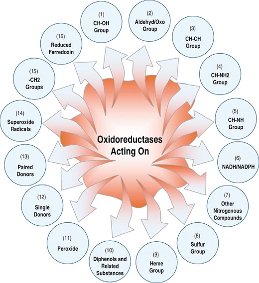
A schematic diagram to show the 16 classes of oxidoreductases classified according to different groups acted by the enzyme.
The success rates in identifying the 16 subfamilies of oxidoreductases with different methods by the self-consistency test
| Subfamily class (Fig. 2) | Number of samplesa | Least Euclidean predictor (Nakashima et al., 1986) (%) | Covariant-discriminant predictor (Chou and Elrod, 2003) (%) | This paperb (%) |
|---|---|---|---|---|
| 1 | 314 | 26.75 | 58.92 | 89.49 |
| 2 | 216 | 50.93 | 64.81 | 87.96 |
| 3 | 194 | 24.23 | 55.67 | 85.57 |
| 4 | 130 | 16.92 | 69.23 | 93.08 |
| 5 | 112 | 12.50 | 65.18 | 83.04 |
| 6 | 305 | 71.80 | 72.79 | 85.57 |
| 7 | 64 | 29.69 | 85.94 | 96.88 |
| 8 | 59 | 23.79 | 96.61 | 100 |
| 9 | 254 | 70.47 | 89.37 | 93.70 |
| 10 | 94 | 42.55 | 67.02 | 95.74 |
| 11 | 154 | 51.95 | 87.66 | 96.75 |
| 12 | 94 | 20.21 | 80.85 | 97.87 |
| 13 | 257 | 70.43 | 79.38 | 96.50 |
| 14 | 155 | 74.19 | 97.42 | 100 |
| 15 | 84 | 79.76 | 96.43 | 100 |
| 16 | 154 | 44.81 | 81.17 | 93.51 |
| Overall | 2640 | 1279/2640 = 48.45% | 1992/2640 = 75.45% | 2433/2640 = 92.16% |
aData taken from Table 1 of Chou and Elrod (2003).
bPerformed using the augmented covariant-discriminant predictor and the Am-Pse-AA composition with λ = 9 and w = 0.5 [Equations (5) and (6)].
The success rates in identifying the 16 subfamilies of oxidoreductases with different methods by the jackknife test
| Subfamily class (Fig. 2) | Number of samplesa | Least Euclidean predictor (Nakashima et al., 1986) (%) | Covariant-discriminant predictor (Chou and Elrod, 2003) (%) | This paperb (%) |
|---|---|---|---|---|
| 1 | 314 | 25.48 | 47.77 | 72.61 |
| 2 | 216 | 49.54 | 54.17 | 66.20 |
| 3 | 194 | 22.68 | 42.78 | 65.46 |
| 4 | 130 | 13.85 | 52.31 | 62.31 |
| 5 | 112 | 8.93 | 44.64 | 47.32 |
| 6 | 305 | 71.48 | 72.13 | 77.70 |
| 7 | 64 | 23.44 | 46.88 | 45.31 |
| 8 | 59 | 16.95 | 52.54 | 23.73 |
| 9 | 254 | 70.08 | 84.65 | 82.28 |
| 10 | 94 | 39.36 | 54.26 | 63.83 |
| 11 | 154 | 51.95 | 78.57 | 81.17 |
| 12 | 94 | 17.02 | 52.13 | 51.06 |
| 13 | 257 | 69.65 | 74.71 | 78.99 |
| 14 | 155 | 71.61 | 93.55 | 92.90 |
| 15 | 84 | 77.38 | 70.24 | 59.52 |
| 16 | 154 | 44.81 | 64.29 | 73.38 |
| Overall | 2640 | 1237/2640 = 46.86% | 1680/2640 = 63.64% | 1864/2640 = 70.61% |
aData taken from Table 1 of Chou and Elrod (2003).
bPerformed using the augmented covariant-discriminant predictor and the Am-Pse-AA composition with λ = 9 and w = 0.5 [Equations (5) and (6)].
The success rates in identifying the 16 subfamilies of oxidoreductasesa by various methods on an independent dataset given in Online Supplementary Materials A
| Subfamily class (Fig. 2) | Number of samplesb | Least Euclidean predictor (Nakashima et al., 1986) (%) | Covariant-discriminant predictor (Chou and Elrod, 2003) (%) | This paperc (%) |
|---|---|---|---|---|
| 1 | 626 | 26.68 | 49.68 | 73.00 |
| 2 | 216 | 47.22 | 57.41 | 70.37 |
| 3 | 25 | 36.00 | 48.00 | 56.00 |
| 4 | 17 | 17.65 | 52.94 | 70.59 |
| 5 | 14 | 7.14 | 50.00 | 50.00 |
| 6 | 608 | 71.38 | 72.37 | 77.30 |
| 7 | 7 | 28.57 | 57.14 | 42.86 |
| 8 | 6 | 33.33 | 50.00 | 50.00 |
| 9 | 253 | 73.91 | 86.17 | 84.58 |
| 10 | 12 | 41.67 | 58.33 | 83.33 |
| 11 | 20 | 50.00 | 75.00 | 90.00 |
| 12 | 12 | 25.00 | 75.00 | 66.67 |
| 13 | 257 | 68.87 | 77.82 | 84.05 |
| 14 | 20 | 70.00 | 90.00 | 95.00 |
| 15 | 11 | 72.73 | 81.82 | 63.64 |
| 16 | 20 | 50.00 | 60.00 | 80.00 |
| Overall | 2124 | 1134/2124 = 53.39% | 1398/2124 = 65.82% | 1626/2124 = 76.55% |
aConducted by the rule parameters derived from the training dataset given in Table 1 of Chou and Elrod (2003).
bData taken from Online Supplementary Materials A.
cPerformed using the augmented covariant-discriminant predictor and the Am-Pse-AA composition with λ = 9 and w = 0.5 [Equations (5) and (6)].
APPENDIX A
For the reader's convenience, here let us prove that the determinant of a non-singular matrix as defined in Equations (12) and (13) is always >0. Without loss of generality, let us simplify Equations (12) and (13) to the following:
where the matrix elements are given by
and
Suppose
thus, we have
where T is the transposition operator, meaning AT is the transposition matrix of A. Suppose
where
is the q-th eigenvector of S, and Λq the corresponding eigenvalue. Since S is a real and symmetric matrix, i.e. S = ST, it follows that its eigenvalues must be a real number, and that the modulus of its eigenvector,
Because the matrix S is non-singular, none of its eigenvalues is 0. It follows by left and right multiplication of both sides of Equation (A5) with
or
Therefore, the determinant of SEquation (A.8) must be >0, and hence ln |S| = ln(Λ1 Λ2 ··· Λu) is always meaningful.
The author wishes to thank the four anonymous reviewers whose comments were very helpful in strengthening the presentation of this study.
REFERENCES
Bahar, I., Atilgan, A.R., Jernigan, R.L., Erman, B.
Bairoch, A. and Apweiler, R.
Cai, Y.D., Li, Y.X., Chou, K.C.
Cedano, J., Aloy, P., P'erez-Pons, J.A., Querol, E.
Chandonia, J.M. and Karplus, M.
Chou, J.J. and Zhang, C.T.
Chou, K.C.
Chou, K.C.
Chou, K.C.
Chou, K.C.
Chou, K.C. and Cai, Y.D.
Chou, K.C. and Zhang, C.T.
Chou, K.C. and Zhang, C.T.
Chou, K.C., Zhang, C.T., Maggiora, M.G.
Chou, P.Y.
Deleage, G. and Roux, B.
Hopp, T.P. and Woods, K.R.
Hua, S. and Sun, Z.
Klein, P.
Klein, P. and Delisi, C.
Kneller, D.G., Cohen, F.E., Langridge, R.
Liu, W. and Chou, K.C.
Mardia, K.V., Kent, J.T., Bibby, J.M.
Metfessel, B.A., Saurugger, P.N., Connelly, D.P., Rich, S.T.
Nakai, K.
Nakai, K. and Kanehisa, M.
Nakashima, H. and Nishikawa, K.
Nakashima, H., Nishikawa, K., Ooi, T.
Pillai, K.C.S.
Tanford, C.
Zhou, G.P.
Zhou, G.P. and Assa-Munt, N.

