


Abstract
The majority of massive stars are in binaries, which implies that many core collapse supernovae should be binaries at the time of the explosion. Here we show that the three most recent, local (visual) SNe (the Crab, Cas A and SN 1987A) were not stellar binaries at death, with limits on the initial mass ratios of q = M2/M1 ≲ 0.1. No quantitative limits have previously been set for Cas A and the Crab, while for SN 1987A we merely updated existing limits in view of new estimates of the dust content. The lack of stellar companions to these three ccSNe implies a 90 per cent confidence upper limit on the q ≳ 0.1 binary fraction at death of fb < 44 per cent. In a passively evolving binary model (meaning no binary interactions), with a flat mass ratio distribution and a Salpeter IMF, the resulting 90 per cent confidence upper limit on the initial binary fraction of F < 63 per cent is in tension with observed massive binary statistics. Allowing a significant fraction fM ≃ 25 per cent of stellar binaries to merge reduces the tension, with |$F < 63({1-f}_{M})^{-1}{\,\rm per\,cent} \simeq 81{\,\rm per\,cent}$|, but allowing for the significant fraction in higher order systems (triples, etc.) reintroduces the tension. That Cas A was not a stellar binary at death also shows that a surviving massive binary companion at the time of the explosion is not necessary for producing a Type IIb SNe. Much larger surveys for binary companions to Galactic SNe will become feasible with the release of the full Gaia proper motion and parallax catalogues providing a powerful probe of the statistics of such binaries and their role in massive star evolution, neutron star velocity distributions and runaway stars.
1 INTRODUCTION
A large fraction of massive stars appear to be in binaries (see the reviews by Duchêne & Kraus 2013 and Moe & Di Stefano 2016). Kobulnicky et al. (2014) estimate that 55 per cent are in binaries with P < 5000 d and mass ratios of 0.2 < q < 1, while Sana et al. (2012) estimate that 69 per cent are in binaries and that two-thirds of these will undergo some form of interaction. Moe & Di Stefano (2016) find that only 16 ± 8 per cent of the 9–16 M⊙ stars that will dominate the SN rate are single and that they have an average multiplicity (companions per primary) of 1.6 ± 0.2.
Mass transfer, mass loss and mergers then significantly modify the subsequent evolution of the system (e.g. Eldridge, Izzard & Tout 2008, Sana et al. 2012). This will, in turn, modify the properties of any resulting supernovae (SNe) over the expectations for isolated stars. For example, the numbers of stripped Type Ibc SNe and the limits on their progenitor stars both suggest that many are stripped through binary mass transfer rather than simply wind (or other) mass loss (e.g. De Donder & Vanbeveren 1998, Eldridge et al. 2008, Smith et al. 2011, Eldridge et al. 2013). There are many theoretical studies exploring the stripped Type IIb, Ib and Ic SNe in the context of binary evolution models (e.g. Yoon, Woosley & Langer 2010, Claeys et al. 2011, Yoon et al. 2012, Dessart et al. 2012, Benvenuto, Bersten & Nomoto 2013, Kim, Yoon & Koo 2015, Yoon, Dessart & Clocchiatti 2017), as well as models for the effects of binary evolution on electron capture SNe (e.g. Moriya & Eldridge 2016).
Discussions of the binary companions to local core collapse SNe (ccSNe) have largely focused on understanding runaway B stars (e.g. Blaauw 1961, Gies & Bolton 1986, Hoogerwerf, de Bruijne & de Zeeuw 2001, Tetzlaff, Neuhäuser & Hohle 2011) and the contribution of binary disruption to the velocities of neutron stars (NS; e.g. Gunn & Ostriker 1970, Iben & Tutukov 1996, Cordes & Chernoff 1998, Faucher-Giguère & Kaspi 2006). van den Bergh (1980) seems to have been the first to search supernova remnants (SNRs) for runaway stars by looking for a statistical excess of O stars close to the centres of 17 SNRs and finding none. Guseinov, Ankay & Tagieva (2005) examined 48 SNRs for O or B stars using simple colour, magnitude and proper motion selection cuts to produce a list of candidates based on the USNO A2 catalogue (Monet et al. 1998). None of these systems have been investigated in any quantitative detail. Dinçel et al. (2015) identify a good candidate in the ∼3 × 10⁴ yr old SNR S147 containing PSR J0538+2817 and argue that it was also likely to have been an interacting binary. Considerably more effort has been devoted to searching for single degenerate companions to Type Ia SN (e.g. Schweizer & Middleditch 1980, Ruiz-Lapuente et al. 2004, Ihara et al. 2007, González Hernández et al. 2012, Schaefer & Pagnotta 2012).
Searches for binary companions to ccSNe in external galaxies are more challenging because the companion is generally significantly fainter than the progenitor (see Kochanek 2009). The Type IIb SN 1993J is probably the best case (Maund et al. 2004, Fox et al. 2014), while the existence of a companion to the Type IIb SN 2011dh is debated, with Folatelli et al. (2014) arguing for a detection and Maund et al. (2015) arguing that the flux may be dominated by late time emission from the SN. There is some evidence of a blue companion for the Type IIb SNe 2001ig (Ryder, Murrowood & Stathakis 2006) and SN 2008ax (Crockett et al. (2008). There are limits on the existence companions to the Type Ic SNe 1994I (Van Dyk, de Mink & Zapartas 2016) and SN 2002ap (Crockett et al. 2007) and the Type IIP SNe 1987A (Graves et al. 2005), SN 2005cs (Maund, Smartt & Danziger 2005, Li et al. 2006) and SN 2008bk (Mattila et al. 2008). All of these limits assume that the SNe made little dust, an issue we discuss further in Kochanek (2017) and consider in more detail for SN 1987A below.
Companions to stripped, Type Ibc SNe can have higher velocities because of the very high progenitor temperatures. For these systems, the finite size of the secondary is important because the radius of the primary is ∼R⊙ and the companion velocities can in theory reach ∼103 km s−1. This is only true if the system was an interacting binary because the orbit of the secondary must also shrink to be far smaller than even the initial size of the primary. Such tightly bound binaries are less likely to be disrupted because the primary mass has to have been greatly reduced by mass loss and the orbital binding energy is larger than typical NS kick velocities (e.g. Cordes & Chernoff 1998). Theoretically, Eldridge et al. (2011), using binary population synthesis models that included such evolutionary paths, found that velocities above 300 km s−1 were very rare.
Here we consider the three most recent visually observed, Local Group, ccSNe: the Crab, Cas A and SN 1987A. For Galactic SN, the Crab and Cas A have several advantages. Their youth means that the search areas are small, and the fact that they were visible by eye means that they have modest extinctions and, by extension, lie in regions with relatively low-stellar densities for the Galaxy. We were unable to find any quantitative discussions of searches for binary companions to these two systems, but Guseinov et al. (2005) report no candidates in their qualitative survey of 48 SNRs. The Crab pulsar is observed in the optical/near-infrared (IR), but it is emission due to the pulsar and not from a surviving binary (e.g. Sandberg & Sollerman 2009, Scott, Finger & Wilson 2003). There have been a series of unsuccessful searches for an optical/near-IR counterpart to the NS in Cas A which rule out any bound system even at the level of a M2 ≃ 0.1 M⊙ dwarf companion (e.g. van den Bergh & Pritchet 1986, Kaplan, Kulkarni & Murray 2001, Ryan, Wagner & Starrfield 2001, Fesen, Pavlov & Sanwal 2006). These studies also implicitly set strong limits on any unbound system, but the topic is never discussed in these papers. Graves et al. (2005) set very strong limits on the existence of a binary companion to SN 1987A but assumed there was very little dust obscuration created by the SN. More recent studies have shown that SN 1987A formed far more dust than assumed by Graves et al. (2005) and that it is concentrated towards the centre of the remnant (Matsuura et al. 2011, Indebetouw et al. 2014, Matsuura et al. 2015), making it necessary to revisit these limits.
The Crab was almost certainly a Type II SNe due to the presence of significant amounts of hydrogen. However, the SNR appears to contain too little mass or energy for it to have been a normal Type II SN suggesting it may have been an electron capture SN [see the review by Hester (2008) or the recent discussion by Smith (2013)]. The binary models of Moriya & Eldridge (2016) would be one way of having such a low-ejecta mass. Cas A is known to be a Type IIb thanks to spectra of light echoes from the SN (Krause et al. 2008, Rest et al. 2008, Rest et al. 2011, Finn et al. 2016). Single star evolution models generally have difficulty producing Type IIb SNe (e.g. Young et al. 2006 for Cas A in particular, Podsiadlowski et al. 1993, Woosley et al. 1994, Claeys et al. 2011, Dessart et al. 2012, Benvenuto et al. 2013, more generally). While SN 1987A was a Type II SN, the progenitor was also a blue rather than a red supergiant (see the review by Arnett et al. 1989). Several models have invoked binary interactions, possibly with a final merger, to explain either the structure of the star or the surrounding winds (e.g. Podsiadlowski & Joss 1989, Podsiadlowski 1992, Blondin & Lundqvist 1993, Morris & Podsiadlowski 2009).
Here we take advantage of the recently released PS1 survey data (hereafter PS1; Chambers et al. 2016) along with their associated three-dimensional maps of dust in the Galaxy (Green et al. 2015) to examine stars near the centres of the Crab and Cas A quantitatively. For consistency with the dust maps, we use the extinction coefficients Aλ from Schlafly & Finkbeiner (2011), which are similar to a standard Galactic RV = 3.1 extinction law. For the Crab and Cas A at these late dates, there will be no significant extinction from dust created by the SN (see Kochanek 2017). We also use, where available, the NOMAD (Zacharias et al. 2005) or HSOY (Altmann et al. 2017) proper motions. We fit the photometry of stars near the centre of the SNR using Solar metallicity stars drawn from the PARSEC isochrones (Bressan et al. 2012). For the coarse luminosity estimates we require the effects of metallicity on stellar colours should not be very important. For SN 1987A we simply examine the consequences of the new dust observations. In Sections 2–4 we discuss the Crab, Cas A and SN 1987A in turn, and we discuss the implications of the results in Section 5.
2 THE CRAB (SN 1054)
Fig. 1 shows the co-added grizy PS1 image of a roughly 2 arcmin region around the centre of the Crab SNR. We adopt an age of 960 yr and, following Kaplan et al. (2008), a distance of 2.0 ± 0.5 kpc or μ = 11.51 ± 0.54 as a distance modulus. Using the Green et al. (2015) dust distribution for the line of sight towards the centre of the SNR, the extinction is roughly E(B − V) ≃ 0.4 mag. Green et al. (2015) estimate that the dust distribution is well-defined out to a distance modulus of 14.2, which is well beyond the distance to the Crab. This extinction estimate agrees well with other determinations (e.g. Wu 1981, Blair et al. 1992). We define the (J2000) centre of the SNR as (05:34:32.84, 22:00:48.0) from Nugent (1998) and the position of the pulsar as (05:34:31.9, 22:00:52.1). Kaplan et al. (2008) measured the proper motion of the pulsar and its estimated position at the time of the SN agrees very closely with the estimated centre of the SNR. The centre of the SNR and the position of the NS at present and in 1054 are both marked in Fig. 1.
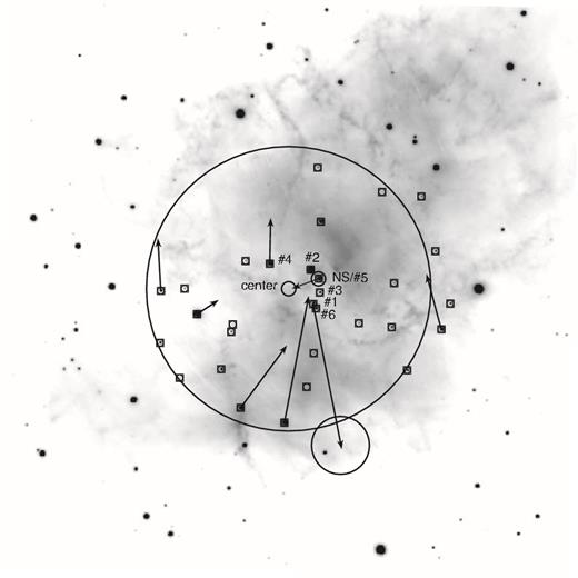
Co-addedgrizy PS1 image of the Crab. The position of the geometric centre of the remnant (‘centre’) and the neutron star are indicated by 3|${^{\prime\prime}_{.}}$|0 radius circles. The larger circle shows the region within 60|${^{\prime\prime}_{.}}$|0 of the centre. The 30 stars within 60|${^{\prime\prime}_{.}}$|0 of either the centre or the NS are marked and the six closest to the centre are numbered in order of their distance from the centre. The NS is star #5. The arrows show the predicted positions of sources with proper motions at the time of the SN. As expected, the predicted position of the pulsar is close to the centre of the SNR. Seven stars have proper motions in NOMAD with uncertainties in their back-projected positions of approximately 12|${^{\prime\prime}_{.}}$|0 as shown by the circle at the head of one of the proper motion vectors. At a distance of 2.0 kpc, a star will have moved 10|${^{\prime\prime}_{.}}$|1(v/100 km s− 1) since the SN, so the 60|${^{\prime\prime}_{.}}$|0 search radius corresponds to a velocity of roughly 600 km s−1.
For a distance of 2.0 kpc and an age of 960 yr, a star with velocity v = 100v2 km s−1 has moved 10|${^{\prime\prime}_{.}}$|1v2. We selected stars within 1 arcmin of either the centre of the SNR or the NS, corresponding to a velocity limit of approximately 600 km s−1. Since the proper motion of the NS only corresponds to v ≃ 100 km s−1 and the Crab is believed to have been a Type II SN (even if peculiar) for which equation (3) applies, only sources within roughly 10|${^{\prime\prime}_{.}}$|0 of the centre can plausibly be surviving secondaries.
The PS1 catalogue for these 1 arcmin regions contains 171 sources, most of which are spurious detections created by the bright nebular emission or faint sources in the wings of the brighter point sources. When we went to fit models to the spectral energy distributions (SEDs) of the actual stars, we frequently found no good fits (χ2 > 100) for any stellar model even though we were using the PS1 point spread function (PSF) magnitudes. This is very different from the case of Cas A (next Section), where we almost always found very good model fits. Presumably this is because the PS1 photometry pipeline was never intended for photometry of stars in a nebular emission region like the centre of the Crab nebula. To remedy this issue, we used sextractor (Bertin & Arnouts 1996) to identify sources on the roughly 2 arcmin square co-added PS1 image and then used iraf aperture photometry with a 3 pixel (0|${^{\prime\prime}_{.}}$|75) aperture radius and a 6 to 10 pixel radius sky aperture. This larger 2 arcmin area includes many stars beyond the brightest nebular regions. We then matched the aperture results to the PS1 photometry and computed the necessary photometric offsets as the median offset after clipping outliers. In the end we had 30 stars to consider, labelled in order of distance from the centre of the SNR, including the NS as star #5. Table 1 provides the positions and grizy aperture magnitudes of these 30 stars along with their distances from the centre of the SNR and the NS.
Stars near the Crab.
| # | dc | dNS | RA | Dec | g | r | i | z | y |
|---|---|---|---|---|---|---|---|---|---|
| 1 | 12|${^{\prime\prime}_{.}}$|1 | 10|${^{\prime\prime}_{.}}$|8 | 83.633 751 | 22.011 540 | 17.875 ± 0.007 | 16.749 ± 0.005 | 16.508 ± 0.005 | 16.232 ± 0.005 | 16.098 ± 0.005 |
| 2 | 12|${^{\prime\prime}_{.}}$|2 | 5|${^{\prime\prime}_{.}}$|6 | 83.634 080 | 22.015 580 | 16.406 ± 0.005 | 15.429 ± 0.004 | 15.102 ± 0.004 | 14.941 ± 0.003 | 14.875 ± 0.004 |
| 3 | 13|${^{\prime\prime}_{.}}$|2 | 5|${^{\prime\prime}_{.}}$|6 | 83.632 910 | 22.012 900 | 20.213 ± 0.041 | 18.479 ± 0.018 | 17.886 ± 0.017 | 17.490 ± 0.009 | 17.114 ± 0.011 |
| 4 | 13|${^{\prime\prime}_{.}}$|2 | 22|${^{\prime\prime}_{.}}$|0 | 83.639 220 | 22.016 270 | 17.145 ± 0.005 | 16.076 ± 0.004 | 15.767 ± 0.003 | 15.870 ± 0.005 | 15.513 ± 0.004 |
| 5 | 13|${^{\prime\prime}_{.}}$|4 | 0|${^{\prime\prime}_{.}}$|5 | 83.633 031 | 22.014 530 | 17.207 ± 0.009 | 16.304 ± 0.009 | 16.088 ± 0.009 | 15.821 ± 0.007 | 15.687 ± 0.009 |
| 6 | 14|${^{\prime\prime}_{.}}$|2 | 12|${^{\prime\prime}_{.}}$|4 | 83.633 381 | 22.011 031 | 18.836 ± 0.011 | 17.822 ± 0.011 | 17.578 ± 0.009 | 17.343 ± 0.009 | 17.163 ± 0.011 |
| 7 | 21|${^{\prime\prime}_{.}}$|6 | 32|${^{\prime\prime}_{.}}$|2 | 83.642 270 | 22.016 590 | 21.955 ± 0.330 | 20.354 ± 0.110 | 18.801 ± 0.029 | 18.147 ± 0.021 | 17.785 ± 0.025 |
| 8 | 28|${^{\prime\prime}_{.}}$|0 | 41|${^{\prime\prime}_{.}}$|3 | 83.643 901 | 22.009 151 | 21.057 ± 0.118 | 19.822 ± 0.053 | 19.412 ± 0.050 | 19.336 ± 0.057 | 19.104 ± 0.099 |
| 9 | 29|${^{\prime\prime}_{.}}$|1 | 31|${^{\prime\prime}_{.}}$|3 | 83.633 680 | 22.005 790 | 22.833 ± 0.327 | 20.526 ± 0.067 | 19.380 ± 0.044 | 19.003 ± 0.030 | 18.544 ± 0.035 |
| 10 | 30|${^{\prime\prime}_{.}}$|3 | 43|${^{\prime\prime}_{.}}$|4 | 83.644 091 | 22.008 290 | 19.849 ± 0.030 | 18.572 ± 0.026 | 18.195 ± 0.013 | 18.019 ± 0.013 | 17.729 ± 0.022 |
| 11 | 31|${^{\prime\prime}_{.}}$|3 | 24|${^{\prime\prime}_{.}}$|3 | 83.632 790 | 22.021 190 | 18.055 ± 0.009 | 16.971 ± 0.005 | 16.813 ± 0.009 | 16.396 ± 0.005 | 16.398 ± 0.007 |
| 12 | 32|${^{\prime\prime}_{.}}$|9 | 24|${^{\prime\prime}_{.}}$|8 | 83.627 980 | 22.009 300 | 20.487 ± 0.066 | 19.226 ± 0.026 | 18.745 ± 0.019 | 18.357 ± 0.018 | 18.355 ± 0.059 |
| 13 | 40|${^{\prime\prime}_{.}}$|1 | 53|${^{\prime\prime}_{.}}$|7 | 83.648 400 | 22.010 360 | 15.976 ± 0.004 | 14.929 ± 0.003 | 14.580 ± 0.003 | 14.377 ± 0.002 | 14.258 ± 0.003 |
| 14 | 42|${^{\prime\prime}_{.}}$|1 | 45|${^{\prime\prime}_{.}}$|7 | 83.634 560 | 22.001 831 | 21.708 ± 0.131 | 20.549 ± 0.103 | 21.173 ± 0.168 | 21.441 ± 0.346 | 20.392 ± 0.264 |
| 15 | 43|${^{\prime\prime}_{.}}$|8 | 57|${^{\prime\prime}_{.}}$|1 | 83.649 970 | 22.013 350 | 19.691 ± 0.019 | 18.806 ± 0.025 | 18.246 ± 0.011 | 18.137 ± 0.015 | 17.996 ± 0.030 |
| 16 | 44|${^{\prime\prime}_{.}}$|3 | 56|${^{\prime\prime}_{.}}$|2 | 83.645 360 | 22.003 920 | 19.306 ± 0.025 | 17.970 ± 0.018 | 17.516 ± 0.009 | 17.264 ± 0.013 | 17.008 ± 0.018 |
| 17 | 44|${^{\prime\prime}_{.}}$|5 | 31|${^{\prime\prime}_{.}}$|4 | 83.623 531 | 22.014 000 | 21.403 ± 0.155 | 19.944 ± 0.095 | 19.034 ± 0.046 | 18.747 ± 0.054 | 18.441 ± 0.064 |
| 18 | 46|${^{\prime\prime}_{.}}$|3 | 36|${^{\prime\prime}_{.}}$|4 | 83.623 841 | 22.008 830 | 19.301 ± 0.043 | 18.178 ± 0.028 | 17.915 ± 0.022 | 17.711 ± 0.013 | 17.572 ± 0.028 |
| 19 | 52|${^{\prime\prime}_{.}}$|5 | 47|${^{\prime\prime}_{.}}$|0 | 83.633 171 | 22.027 510 | 21.674 ± 0.130 | 19.710 ± 0.029 | 18.614 ± 0.024 | 18.098 ± 0.017 | 17.837 ± 0.021 |
| 20 | 53|${^{\prime\prime}_{.}}$|9 | 67|${^{\prime\prime}_{.}}$|1 | 83.652 970 | 22.013 090 | 18.549 ± 0.013 | 17.471 ± 0.011 | 16.953 ± 0.009 | 16.819 ± 0.009 | 16.612 ± 0.013 |
| 21 | 54|${^{\prime\prime}_{.}}$|1 | 63|${^{\prime\prime}_{.}}$|6 | 83.642 910 | 21.999 390 | 17.840 ± 0.011 | 16.788 ± 0.011 | 16.540 ± 0.007 | 16.369 ± 0.005 | 16.098 ± 0.009 |
| 22 | 56|${^{\prime\prime}_{.}}$|5 | 62|${^{\prime\prime}_{.}}$|2 | 83.637 380 | 21.997 660 | 16.915 ± 0.005 | 15.841 ± 0.004 | 15.490 ± 0.005 | 15.354 ± 0.004 | 15.119 ± 0.005 |
| 23 | 56|${^{\prime\prime}_{.}}$|7 | 45|${^{\prime\prime}_{.}}$|2 | 83.625 051 | 22.024 660 | 21.395 ± 0.129 | 20.314 ± 0.137 | 19.727 ± 0.071 | 19.585 ± 0.075 | 19.326 ± 0.088 |
| 24 | 58|${^{\prime\prime}_{.}}$|8 | 72|${^{\prime\prime}_{.}}$|4 | 83.653 070 | 22.007 001 | 19.107 ± 0.013 | 17.892 ± 0.007 | 17.595 ± 0.009 | 17.162 ± 0.007 | 17.182 ± 0.015 |
| 25 | 59|${^{\prime\prime}_{.}}$|3 | 72|${^{\prime\prime}_{.}}$|2 | 83.650 590 | 22.002 890 | 20.473 ± 0.041 | 19.430 ± 0.040 | 19.089 ± 0.036 | 18.953 ± 0.036 | 18.766 ± 0.054 |
| 26 | 60|${^{\prime\prime}_{.}}$|6 | 53|${^{\prime\prime}_{.}}$|2 | 83.621 881 | 22.003 800 | 19.146 ± 0.015 | 18.085 ± 0.009 | 17.933 ± 0.009 | 17.620 ± 0.009 | 17.480 ± 0.013 |
| 27 | 63|${^{\prime\prime}_{.}}$|8 | 50|${^{\prime\prime}_{.}}$|2 | 83.618 310 | 22.017 740 | 19.334 ± 0.018 | 18.261 ± 0.026 | 17.996 ± 0.015 | 17.825 ± 0.015 | 17.564 ± 0.021 |
| 28 | 66|${^{\prime\prime}_{.}}$|5 | 55|${^{\prime\prime}_{.}}$|4 | 83.617 581 | 22.008 580 | 17.723 ± 0.007 | 16.672 ± 0.005 | 16.724 ± 0.007 | 16.229 ± 0.005 | 16.051 ± 0.007 |
| 29 | 68|${^{\prime\prime}_{.}}$|1 | 55|${^{\prime\prime}_{.}}$|2 | 83.620 091 | 22.024 130 | 21.746 ± 0.236 | 19.173 ± 0.086 | 18.695 ± 0.018 | 18.258 ± 0.015 | 17.765 ± 0.030 |
| 30 | 68|${^{\prime\prime}_{.}}$|3 | 55|${^{\prime\prime}_{.}}$|9 | 83.616 450 | 22.011 591 | 18.793 ± 0.017 | 18.011 ± 0.018 | 17.899 ± 0.011 | 17.694 ± 0.009 | 17.448 ± 0.017 |
The stars are numbered in order of their distance from the centre of the SNR (dc) and the distance from the NS (dNS) is also given.
The magnitudes are aperture magnitudes found from the PS1 images and an entry of − indicates no detection.
There are, in fact, no sources closer than 12|${^{\prime\prime}_{.}}$|0 to the centre of the SNR. Since there is so little ambiguity in the centre given its close (arcsec) agreement with the proper motion of the pulsar, and even a 10|${^{\prime\prime}_{.}}$|0 search radius is already generous for the companion of a Type II SN, we can immediately rule out the existence of a binary companion with M2 ≳ M⊙ simply from the structure of the colour magnitude diagram (CMD). This could be strengthened further using the still deeper HubbleSpaceTelescope data. There are six sources between 12|${^{\prime\prime}_{.}}$|0 and 15|${^{\prime\prime}_{.}}$|0, where the pulsar is source #5, and then the next source is 21|${^{\prime\prime}_{.}}$|7 from the centre. We number the sources by their distance from the centre of the SNR and have labelled only the six closest sources in Fig. 1.
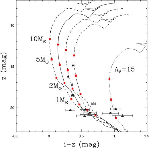
Fig. 2 shows the r/r−i CMD of these sources. Superposed are the PARSEC isochrones for Solar metallicity stars with an age of 107.3 yr, roughly corresponding to the epoch at which 12 M⊙ stars would die, along with the effects of changing the extinction estimates to E(B − V) = 0 or 0.9 mag. The distance uncertainties are much less important, since they only correspond to shifting the isochrone vertically by ±0.5 mag. Like Guseinov et al. (2005), we find no plausible candidates for a former binary companion.
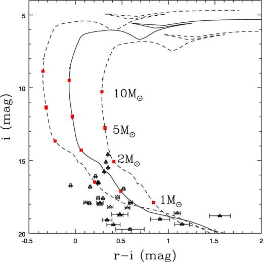
The r/r−i CMD of the stars within 60|${^{\prime\prime}_{.}}$|0 of the centre of the Crab SNR or NS. The solid curve shows the PARSEC (Bressan et al. 2012) isochrone for Solar metallicity stars with an age of 107.3 yr at a distance of 2 kpc and with an extinction of E(B − V) = 0.4 mag. The dashed curves show the effect of reducing (raising) the extinction to E(B − V) = 0 mag (0.9 mag). Uncertainties in the distance modulus are much less important corresponding to vertical shifts of ±0.5 mag. Red filled squares on the isochrones mark stars with masses of 1, 2, 5 and 10 M⊙.
Seven of the stars (#1, #4, #13, #20, #21, #22 and #28) have proper motions in the NOMAD catalogue and their predicted positions at the time of the SN are indicated by the arrows in Fig. 1. The uncertainties in the proper motions lead to a position uncertainty of approximately 12|${^{\prime\prime}_{.}}$|0 after 960 yr, as indicated by the circle at the end of one of the proper motion vectors. Only the distant star #22 has a proper motion consistent with the position of the SN, but it would also have to be moving at almost 600 km s−1. The two closer stars with proper motions, #1 and #4, are moving in the wrong direction to be associated with the SN.
Fits to stars near the Crab.
| # | |$\chi ^2_0$| | |$\chi ^2_1$| | |$\chi ^2_2$| | log L1/L⊙ | log T1 | log L2/L⊙ | log T2 |
|---|---|---|---|---|---|---|---|
| 1 | 5.5 | 6.0 | 8.1 | |$\hphantom{-}0.06\pm 0.25$| | 3.672 ± 0.030 | |$\hphantom{-}0.17\pm 0.30$| | 3.711 ± 0.004 |
| 2 | 0.1 | 0.9 | 3.9 | |$\hphantom{-}0.44\pm 0.24$| | 3.681 ± 0.024 | |$\hphantom{-}0.67\pm 0.20$| | 3.736 ± 0.004 |
| 3 | 9.8 | 10.3 | 26.6 | −0.11 ± 0.33 | 3.676 ± 0.037 | −0.65 ± 0.47 | 3.602 ± 0.005 |
| 4 | 21.9 | 23.6 | 30.7 | |$\hphantom{-}0.28\pm 0.48$| | 3.716 ± 0.074 | |$\hphantom{-}0.27\pm 0.49$| | 3.740 ± 0.009 |
| 5 | 3.6 | 5.6 | 5.7 | |$\hphantom{-}0.40\pm 0.32$| | 3.764 ± 0.067 | |$\hphantom{-}0.35\pm 0.26$| | 3.745 ± 0.004 |
| 6 | 24.9 | 30.9 | 31.0 | |$\hphantom{-}0.04\pm 0.55$| | 3.748 ± 0.077 | −0.17 ± 0.28 | 3.730 ± 0.008 |
| 7 | 0.1 | 0.5 | 0.7 | −0.57 ± 0.23 | 3.545 ± 0.021 | −0.67 ± 0.19 | 3.533 ± 0.003 |
| 8 | 5.1 | 9.5 | 16.7 | −0.71 ± 0.17 | 3.659 ± 0.021 | −0.37 ± 0.12 | 3.716 ± 0.008 |
| 9 | 13.5 | 14.3 | 17.8 | −0.41 ± 0.47 | 3.686 ± 0.069 | −0.97 ± 0.35 | 3.566 ± 0.004 |
| 10 | 17.8 | 19.2 | 19.9 | −0.41 ± 0.37 | 3.688 ± 0.046 | −0.50 ± 0.24 | 3.681 ± 0.005 |
| 11 | 12.7 | 15.0 | 16.8 | |$\hphantom{-}0.04\pm 0.39$| | 3.709 ± 0.057 | −0.04 ± 0.38 | 3.721 ± 0.006 |
| 12 | 8.2 | 10.1 | 10.5 | −0.62 ± 0.30 | 3.666 ± 0.040 | −0.61 ± 0.16 | 3.668 ± 0.003 |
| 13 | 0.5 | 1.8 | 2.5 | |$\hphantom{-}0.81\pm 0.23$| | 3.703 ± 0.020 | |$\hphantom{-}0.82\pm 0.18$| | 3.712 ± 0.003 |
| 14 | 26.1 | 54.1 | 79.9 | −0.29 ± 0.42 | 3.714 ± 0.052 | |$\hphantom{-}0.05\pm 0.22$| | 3.762 ± 0.016 |
| 15 | 8.7 | 10.0 | 11.5 | −0.37 ± 0.32 | 3.706 ± 0.045 | −0.36 ± 0.11 | 3.715 ± 0.004 |
| 16 | 3.6 | 3.8 | 3.9 | −0.25 ± 0.23 | 3.667 ± 0.025 | −0.23 ± 0.24 | 3.662 ± 0.002 |
| 17 | 6.9 | 7.1 | 7.4 | −0.71 ± 0.38 | 3.650 ± 0.055 | −0.93 ± 0.14 | 3.610 ± 0.002 |
| 18 | 15.6 | 18.0 | 21.1 | −0.40 ± 0.35 | 3.691 ± 0.043 | −0.29 ± 0.19 | 3.719 ± 0.006 |
| 19 | 23.6 | 27.6 | 32.8 | |$\hphantom{-}0.04\pm 0.64$| | 3.736 ± 0.096 | −0.83 ± 0.40 | 3.564 ± 0.006 |
| 20 | 1.9 | 1.9 | 2.1 | −0.11 ± 0.25 | 3.685 ± 0.051 | −0.06 ± 0.23 | 3.691 ± 0.003 |
| 21 | 9.1 | 9.5 | 10.9 | |$\hphantom{-}0.12\pm 0.35$| | 3.716 ± 0.063 | |$\hphantom{-}0.05\pm 0.36$| | 3.722 ± 0.005 |
| 22 | 3.7 | 4.3 | 5.7 | |$\hphantom{-}0.39\pm 0.23$| | 3.682 ± 0.027 | |$\hphantom{-}0.56\pm 0.21$| | 3.710 ± 0.003 |
| 23 | 2.0 | 4.9 | 8.4 | −0.89 ± 0.19 | 3.629 ± 0.024 | −0.63 ± 0.08 | 3.676 ± 0.003 |
| 24 | 8.2 | 11.9 | 12.6 | −0.29 ± 0.34 | 3.686 ± 0.044 | −0.32 ± 0.31 | 3.689 ± 0.005 |
| 25 | 3.2 | 6.0 | 12.4 | −0.70 ± 0.16 | 3.662 ± 0.019 | −0.29 ± 0.11 | 3.726 ± 0.007 |
| 26 | 22.3 | 26.1 | 27.4 | −0.18 ± 0.46 | 3.720 ± 0.059 | −0.20 ± 0.22 | 3.731 ± 0.007 |
| 27 | 17.7 | 20.3 | 21.6 | −0.29 ± 0.40 | 3.709 ± 0.051 | −0.28 ± 0.20 | 3.721 ± 0.007 |
| 28 | 37.2 | 46.4 | 46.9 | |$\hphantom{-}0.70\pm 0.78$| | 3.828 ± 0.135 | |$\hphantom{-}0.15\pm 0.50$| | 3.736 ± 0.012 |
| 29 | 28.3 | 28.6 | 45.2 | |$\hphantom{-}0.04\pm 0.59$| | 3.737 ± 0.088 | −0.87 ± 0.42 | 3.592 ± 0.004 |
| 30 | 18.1 | 27.5 | 29.9 | |$\hphantom{-}0.07\pm 0.54$| | 3.765 ± 0.071 | |$\hphantom{-}0.22\pm 0.20$| | 3.785 ± 0.011 |
The ID numbers are the same as in Table 1. The goodnesses of fit |$\chi ^2_0$|, |$\chi ^2_1$| and |$\chi ^2_2$| are for fits with no prior, a prior for the distance to the SN and a prior on both the distance and the extinction. The probability weighted mean luminosities and temperatures are reported for the latter two models.
As is typical of trying to estimate stellar distances using only photometry, it is nearly impossible to do so without additional constraints. Very few of the stars cannot be placed at the distance of the Crab if there is no constraint on the extinction (5 of 30 have |$\chi ^2_1 > \chi ^2_0 + 4$|). With the addition of the constraint on the extinction at any given distance included, many fewer have solutions consistent with the distance (15 of 30 have |$\chi ^2_2 > \chi ^2_0 + 4$|), but that still leaves many that are consistent with both priors. Curiously, the non-thermal emission of the NS (#5) can be well-modelled by a stellar SED.
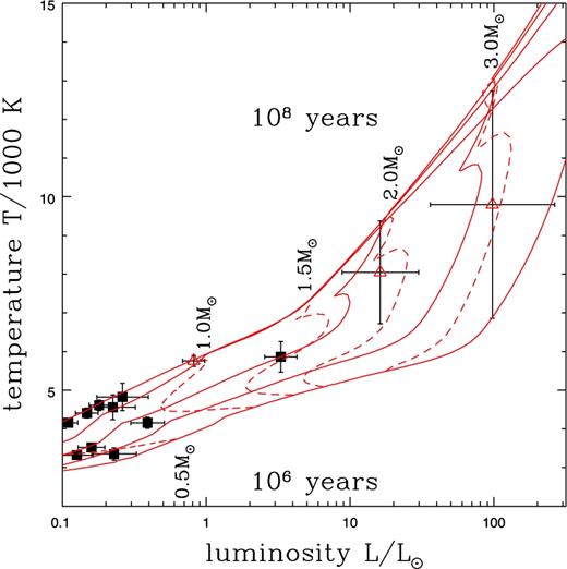
Fig. 3 shows the luminosities and temperatures the stars would have at the distance of the Crab and with the extinction prior (|$\chi ^2_2$|). The distribution looks similar without the extinction prior, but the uncertainties, particularly the temperature uncertainties, become larger (see Table 2). If any of these stars are at the distance of the Crab, none of them are either luminous or massive. Moreover, many of the more luminous stars are also the ones with proper motions, almost all of which are inconsistent with an association with SN 1054. More importantly, an actual companion to the Crab SN would have to be closer to the centre of the SNR where no stars of similar magnitudes are observed. This implies that the Crab had no stellar companion to even stricter limits of L ≲ L⊙ and M ≲ M⊙ even if we are very conservative.
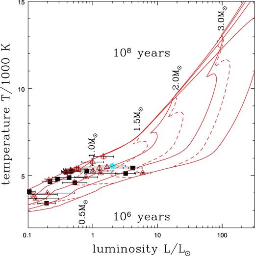
The luminosities and temperatures of the stars if at the distance of the Crab and constrained by the extinction prior. Filled black squares mark the stars that could be at the distance of the Crab (|$\chi _2^2 < \chi ^2_0 + 4$|) and an association is not ruled out by the available proper motions. Open red triangles are for stars that either cannot lie at the distance of the Crab (|$\chi _2^2 > \chi ^2_0 + 4$|) or have a proper motion inconsistent with an association. The pulsar, fit as a star, is indicated by the filled, cyan pentagon. The solid lines show isochrones with ages of 106, 106.5, 107, 107.5 and 108 yr while the dashed lines show the tracks for 0.5, 1.0, 1.5, 2.0 and 3.0 M⊙ stars over this range of times.
3 CASSIOPEIA A
Fig. 4 shows the co-added grizy PS1 image of a roughly 2 arcmin region centred on Cas A. The emission lines present in some of the bands show an outline of the remnant, and we have marked the geometric centre (23:23:27.82, 58:48:49.4) of the remnant (Thorstensen, Fesen & van den Bergh 2001) and the position of the neutron star (23:23:27.93, 58:48:42.5). We adopt a distance of 3.4 ± 0.3 kpc (Reed et al. 1995) and an age of 330 yr. For this distance, a source with velocity 100v2 km s−1 will have moved 2|${^{\prime\prime}_{.}}$|0v2 in the 330 yr since the SN. The 7|${^{\prime\prime}_{.}}$|0 distance of the NS from the centre of the SNR corresponds to a velocity of approximately 340 km s−1.
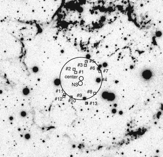
Co-addedgrizy PS1 image of Cas A. The position of the geometric centre of the remnant (‘centre’) and the neutron star are indicated by 3|${^{\prime\prime}_{.}}$|0 radius circles. The larger circle shows the region within 30|${^{\prime\prime}_{.}}$|0 of the centre. The 13 PS1 stars lying within 30|${^{\prime\prime}_{.}}$|0 of either the geometric centre or the neutron star are marked and labelled in order of their distance from the centre. None of the stars have proper motion measurements in NOMAD. Stars #4, #9 and #13 have proper motions in HSOY but the shift in position to the time of the SN is too small to display. At a distance of 3.4 kpc, a star will have moved 2|${^{\prime\prime}_{.}}$|1(v/100 km s− 1) since the SN, so the 30|${^{\prime\prime}_{.}}$|0 search radius corresponds to a velocity of roughly 1500 km s−1
The PS1 extinction estimate at the distance of Cas A is E(B − V) ≃ 1.2 (AV = 3.7), but it lies close to a sudden jump in the extinction to E(B − V) ≃ 1.5 (AV = 4.7). This is more consistent with early estimates of AV ≃ 4.3 mag by Searle (1971) and lower than the estimates of AV ≃ 5.3–6.2 mag by Hurford & Fesen (1996) and AV = 6.2 ± 0.6 mag by Eriksen et al. (2009). These estimates are based on using predicted and observed SNR emission line ratios to determine the extinction. The distances used in the PS1 extinction estimates are only reliable out to Cas A.
We used a generous selection radius of 30|${^{\prime\prime}_{.}}$|0 from either the centre of the SNR or the NS, which corresponds to a velocity of almost 1500 km s−1. These regions contain 15 PS1 sources of which two are obvious artefacts. This leaves thirteen stars, which we have again labelled in order of their distance from the centre of the SNR as shown in Fig. 4 and reported in Table 3. None of the stars have proper motion estimates in NOMAD and three (#4, #9 and #13) have proper motions in HSOY. The predicted positions of these three stars at the time of the SN are within a few arcsec of their present positions and are too small to display in Fig. 4. They cannot have been associated with the SN.
Stars near Cas A.
| # | dc | dNS | RA | Dec | g | r | i | z | y |
|---|---|---|---|---|---|---|---|---|---|
| 1 | 11|${^{\prime\prime}_{.}}$|7 | 16|${^{\prime\prime}_{.}}$|9 | 350.869 920 | 58.816 130 | 26.968 ± 6.896 | 22.959 ± 0.243 | 21.610 ± 0.085 | 21.066 ± 0.096 | 20.460 ± 0.127 |
| 2 | 16|${^{\prime\prime}_{.}}$|6 | 21|${^{\prime\prime}_{.}}$|9 | 350.871 040 | 58.817 400 | 24.223 ± 0.478 | 22.431 ± 0.153 | 21.512 ± 0.089 | 20.907 ± 0.093 | 20.540 ± 0.143 |
| 3 | 19|${^{\prime\prime}_{.}}$|8 | 26|${^{\prime\prime}_{.}}$|7 | 350.862 510 | 58.818 970 | – | 23.087 ± 0.241 | 21.694 ± 0.102 | 20.755 ± 0.072 | 20.069 ± 0.086 |
| 4 | 23|${^{\prime\prime}_{.}}$|8 | 25|${^{\prime\prime}_{.}}$|3 | 350.853 010 | 58.813 060 | 16.802 ± 0.003 | 15.775 ± 0.003 | 15.306 ± 0.003 | 14.939 ± 0.003 | 14.712 ± 0.003 |
| 5 | 25|${^{\prime\prime}_{.}}$|3 | 32|${^{\prime\prime}_{.}}$|2 | 350.861 801 | 58.820 450 | 23.675 ± 0.290 | 22.005 ± 0.119 | 20.701 ± 0.051 | 20.375 ± 0.051 | 19.764 ± 0.066 |
| 6 | 28|${^{\prime\prime}_{.}}$|0 | 32|${^{\prime\prime}_{.}}$|9 | 350.852 650 | 58.817 580 | 19.784 ± 0.009 | 18.349 ± 0.007 | 17.633 ± 0.005 | 17.278 ± 0.007 | 17.003 ± 0.009 |
| 7 | 28|${^{\prime\prime}_{.}}$|3 | 24|${^{\prime\prime}_{.}}$|7 | 350.855 350 | 58.807 990 | 26.995 ± 4.898 | 23.297 ± 0.335 | 22.169 ± 0.126 | 21.046 ± 0.096 | 20.221 ± 0.110 |
| 8 | 28|${^{\prime\prime}_{.}}$|5 | 32|${^{\prime\prime}_{.}}$|6 | 350.851 430 | 58.816 520 | 24.604 ± 0.551 | 22.601 ± 0.194 | 21.244 ± 0.066 | 20.224 ± 0.050 | 19.396 ± 0.046 |
| 9 | 28|${^{\prime\prime}_{.}}$|5 | 22|${^{\prime\prime}_{.}}$|0 | 350.863 360 | 58.805 910 | 18.290 ± 0.004 | 17.258 ± 0.004 | 16.596 ± 0.003 | 16.304 ± 0.004 | 16.072 ± 0.004 |
| 10 | 29|${^{\prime\prime}_{.}}$|6 | 23|${^{\prime\prime}_{.}}$|1 | 350.873 351 | 58.806 511 | 23.511 ± 0.237 | 21.663 ± 0.069 | 20.273 ± 0.026 | 19.595 ± 0.018 | 19.317 ± 0.038 |
| 11 | 32|${^{\prime\prime}_{.}}$|4 | 27|${^{\prime\prime}_{.}}$|1 | 350.878 290 | 58.807 510 | 24.849 ± 0.694 | 22.528 ± 0.179 | 21.322 ± 0.074 | 20.694 ± 0.062 | 20.674 ± 0.186 |
| 12 | 34|${^{\prime\prime}_{.}}$|9 | 29|${^{\prime\prime}_{.}}$|4 | 350.878 871 | 58.806 840 | 23.770 ± 0.284 | 22.723 ± 0.270 | 20.867 ± 0.043 | 20.308 ± 0.042 | 19.909 ± 0.076 |
| 13 | 35|${^{\prime\prime}_{.}}$|5 | 29|${^{\prime\prime}_{.}}$|2 | 350.861 641 | 58.804 091 | 20.880 ± 0.018 | 19.655 ± 0.011 | 18.956 ± 0.007 | 18.598 ± 0.011 | 18.278 ± 0.015 |
The stars are numbered in order of their distance from the centre of the SNR (dc) and the distance from the NS (dNS) is also given. The magnitudes are aperture magnitudes found from the PS1 images and an entry of – indicates no detection.
The closest star (#1) lies 11|${^{\prime\prime}_{.}}$|5 from the centre of the SNR and 16|${^{\prime\prime}_{.}}$|7 from the NS, corresponding to velocities of 560 and 820 km s−1 that are not physical for the companion of a Type II (IIb) SN. The NS, while an X-ray source, is not detected to very deep optical/near-IR limits (≳28 mag at R band, Fesen et al. 2006). We again replaced the PS1 magnitudes with the results of aperture photometry. Here nebulosity is not an issue and the PS1 PSF photometry produces good fits. However, replacing the PS1 PSF photometry with forced aperture photometry allowed us to include photometry in more bands than PS1 reports due to limits on signal-to-noise ratios.
Fig. 5 shows the z/i−z CMD of the stars. The brighter and closer (to the centre) stars are labelled. Stars such as #4, #6 and #9 which could have M > M⊙ at the distance of Cas A (and assuming more extinction than the PS1 model) are at least 24|${^{\prime\prime}_{.}}$|0 from the centre or the NS and would require v ≳ 1200 km s−1 to be associated with the SN. Three of the four brightest stars (#4, #9 and #13) are also ruled out by their HSOY proper motions. There is no proper motion information for #6. The two closest PS1 stars would have to be M ≲ M⊙ and still require unreasonably high velocities.
The z/i−z CMD of the stars within 30|${^{\prime\prime}_{.}}$|0 of the centre of the Cas A SNR or the NS. The solid curve shows the PARSEC (Bressan et al. 2012) isochrone for Solar metallicity stars with an age of 107.3 yr at a distance of 3.4 kpc and with an extinction of E(B − V) = 1.6 mag (AV = 5.0). The dashed curves show the effect of reducing the extinction to AV = 3.4 or raising it to 6.5 or 8.0 mag. The dotted curve shows the effect of assuming a very high extinction of AV = −15 mag. Uncertainties in the distance modulus are much less important corresponding to vertical shifts of ±0.2 mag. Red filled squares on the isochrones mark stars with masses of 1, 2, 5 and 10 M⊙.
Table 4 presents the results of fitting stellar models to the SEDs. Most of the stars can be well-fit, with star #5 as the worst case. We again find that roughly half the stars have properties consistent with the distance and extinction of Cas A. Fig. 6 shows the luminosities and temperatures of the stars including the extinction prior. As suggested by the CMD, stars #4, #6 and #9 can have the highest luminosities, with #4 potentially being a ≃3 M⊙ B star with L ≃ 102.0 L⊙. However, #4 and #9 also have HSOY proper motions inconsistent with any association. The rest of the stars would be low-mass (M < M⊙) dwarfs. As with the Crab, even these low-mass stars are absent at distances from the centre corresponding to reasonable velocities, so it is clear that any binary companion to Cas A at death would have to have M ≲ M⊙.
The luminosities and temperatures of the stars if at the distance of the Cas A and constrained by the extinction prior. Filled black squares mark the stars that could be at the distance of Cas A (|$\chi _2^2 < \chi ^2_0 + 4$|) and not ruled out by proper motions. Open red triangles mark stars that cannot be at the distance of Cas A (|$\chi _2^2 > \chi ^2_0 + 4$|) or an association is ruled out by the proper motions. In practice, the only star which is inconsistent with the distance (#13) is also ruled out by its proper motion. The solid lines show isochrones with ages of 106, 106.5, 107, 107.5 and 108 yr while the dashed lines show the tracks for 0.5, 1.0, 1.5, 2.0 and 3.0 M⊙ stars over this range of times.
Fits to stars near Cas A.
| # | |$\chi ^2_0$| | |$\chi ^2_1$| | |$\chi ^2_2$| | log L1/L⊙ | log T1 | log L2/L⊙ | log T2 |
|---|---|---|---|---|---|---|---|
| 1 | 1.5 | 2.0 | 2.1 | −0.81 ± 0.30 | 3.635 ± 0.052 | −0.91 ± 0.12 | 3.619 ± 0.010 |
| 2 | 0.2 | 1.3 | 3.2 | −1.08 ± 0.25 | 3.598 ± 0.032 | −0.70 ± 0.12 | 3.664 ± 0.013 |
| 3 | 0.7 | 2.2 | 5.9 | −0.07 ± 0.22 | 3.738 ± 0.051 | −0.75 ± 0.14 | 3.547 ± 0.009 |
| 4 | 0.6 | 1.5 | 1.6 | |$\hphantom{-}2.26\pm 0.50$| | 4.074 ± 0.152 | |$\hphantom{-}2.04\pm 0.48$| | 3.992 ± 0.131 |
| 5 | 15.3 | 17.4 | 17.6 | −0.61 ± 0.33 | 3.660 ± 0.062 | −0.53 ± 0.23 | 3.684 ± 0.032 |
| 6 | 0.3 | 0.4 | 1.8 | |$\hphantom{-}0.44\pm 0.17$| | 3.703 ± 0.041 | |$\hphantom{-}0.57\pm 0.16$| | 3.768 ± 0.030 |
| 7 | 3.2 | 5.7 | 10.9 | −0.00 ± 0.28 | 3.741 ± 0.061 | −0.85 ± 0.16 | 3.522 ± 0.014 |
| 8 | 8.7 | 16.4 | 30.6 | |$\hphantom{-}0.50\pm 0.37$| | 3.806 ± 0.076 | −0.59 ± 0.21 | 3.526 ± 0.021 |
| 9 | 0.2 | 0.8 | 0.9 | |$\hphantom{-}1.28\pm 0.34$| | 3.913 ± 0.094 | |$\hphantom{-}1.26\pm 0.32$| | 3.906 ± 0.072 |
| 10 | 2.9 | 3.6 | 7.6 | −0.65 ± 0.15 | 3.558 ± 0.014 | −0.36 ± 0.17 | 3.619 ± 0.015 |
| 11 | 2.8 | 3.4 | 4.1 | −0.93 ± 0.29 | 3.614 ± 0.048 | −0.78 ± 0.13 | 3.645 ± 0.013 |
| 12 | 2.3 | 3.7 | 9.5 | −1.06 ± 0.17 | 3.523 ± 0.027 | −0.60 ± 0.21 | 3.659 ± 0.031 |
| 13 | 4.1 | 7.2 | 9.4 | |$\hphantom{-}0.06\pm 0.17$| | 3.770 ± 0.022 | −0.04 ± 0.13 | 3.761 ± 0.011 |
The ID numbers are the same as in Table 3. The goodnesses of fit |$\chi ^2_0$|, |$\chi ^2_1$|, and |$\chi ^2_2$| are for fits with no prior, a prior for the distance to the SN and a prior on both the distance and the extinction. The probability weighted mean luminosities and temperatures are reported for the latter two models.
De Looze et al. (2017) suggest that the extinction towards Cas A could be significantly higher than that found in the Green et al. (2015) extinction models, reaching AV = 15 mag. Fig. 5 also shows the position of the isochrone shifted to this higher extinction. Most of the PS1 stars in the field are far too blue to be so heavily extincted, but stars #3, #7 and #8 are sufficiently red. These are all sufficiently distant from the centre that they are unlikely to be surviving companions. Star #3, the closest, lies 19|${^{\prime\prime}_{.}}$|8 from the centre, corresponding to a velocity of almost 1000 km s−1. However, Fig. 5 also shows that the detection limit for the PS1 catalogues rises to roughly 2 M⊙ at such high extinctions. While weaker, this is still a relatively tight constraint.
Fortunately, Fesen et al. (2006) provide deep HubbleSpaceTelescope photometry for a region encompassing companion velocities of up to 300 km s−1 relative to the centre of the SNR. They find only three faint sources, which they label stars A (1|${^{\prime\prime}_{.}}$|8), B (1|${^{\prime\prime}_{.}}$|9) and C (3|${^{\prime\prime}_{.}}$|6), none of which correspond to the NS. If we model these three sources following the same procedures as used for the PS1 sources, the upper limits on their masses even at the high extinctions advocated by De Looze et al. (2017) are again constrained to be M ≲ M⊙.
4 SN 1987A
Graves et al. (2005) obtained very tight limits on the presence of an optical point source at the centre of SN 1987A, with limits of νLν < 0.26, 0.33, 0.15, 0.30 and 0.28 L⊙ in the F330W, F435W, F555W, F625W and F814W filters. To account for dust absorption in their estimates, they note that the fraction of the bolometric luminosity emerging in the infrared on day 2172 was 97 per cent (Bouchet & Danziger 1993) implying an effective optical depth of τ ≃ 3.5. The effective optical depth at the time of their observations (day 6110) would then be τ = 0.45 because of the 1/t2 dilution of the optical depth due to expansion. This then implies that there cannot be a binary companion (or other point source) more luminous than roughly L < 2 L⊙.
Graves et al. (2005) discuss scenarios in which the dust might be clumped, but these scenarios were based on clumpy dust distributions in a foreground screen rather than a circumstellar medium. For a clumpy medium closely surrounding the source, the extra absorption from a clump that happens to be along our line of sight will be partially balanced by the contribution from photons scattered on to our line of sight by other clumps (see the discussion in Kochanek, Khan & Dai 2012). This would essentially eliminate the worst case scenario they consider, where there would be no dilution of the optical depth by expansion and the luminosity constraint would be ∼30 times weaker.
As a result, it is really only the mid-IR dust emission which constrains the luminosity of any central source. Matsuura et al. (2015) find a total central dust luminosity in 2012 of 230 L⊙. This luminosity is due to a combination of radioactive decay, absorption of radiation from the expanding shocks and any contribution from a central source. Matsuura et al. (2015) estimate that the available heating from decay of 44Ti is ≃ 400 L⊙, extrapolating from Jerkstrand, Fransson & Kozma (2011), and that a further ∼50 L⊙ can be heating from the shocks exterior to the dusty region. They do not discuss any additional contributions, but the two required heating sources already exceed the observed luminosity, which suggests that only a modest fraction of the observed 230 L⊙ could be due to a binary companion. A reasonable upper limit is probably 10 per cent of the total luminosity, which corresponds to M ≲ 2.5 M⊙ (see Fig. 6). A 3 M⊙ companion would already represent half the observed luminosity.
5 DISCUSSION
Examining the PS1 sources near the Crab and Cas A, it is clear that these SN had no binary companion at death with a mass M ≳ M⊙. Graves et al. (2005) found a similar limit for SN 1987A, but the higher present day estimates of the dust content imply a weaker limit of M ≲ 2.5 M⊙ from the observed dust luminosity. In terms of mass ratios, there are no companions to these three ccSNe with initial mass ratios above q ≳ 0.1. This assumes that the progenitors of Cas A and the Crab were ≳8 M⊙ and that the progenitor of SN 1987A was ∼20 M⊙ (e.g. Weiss, Hillebrandt & Truran 1988, Tuchman & Wheeler 1989, Podsiadlowski, Joss & Rappaport 1990). If the progenitors are merger remnants, as is proposed for SN 1987A, then the limits are really on the presence of a tertiary and (roughly) correspond to limiting any tertiaries to q ≲ 0.2 relative to the pre-merger primary. If the binary fraction at death is fb, the probability of finding no binaries companions in three systems is (1 − fb)3 implying that fb < 0.44 at 90 per cent confidence.
These results may not be surprising for the Crab and SN 1987A. The Crab lies well off the Galactic plane, suggesting that its progenitor was a runaway OB star (Minkowski 1970, Trimble & Rees 1971). This would likely mean that the Crab was the explosion of the secondary star from a binary disrupted in an earlier explosion. As discussed in the introduction, many models for SN 1987A invoke binary interactions with a final merger to explain the properties of the SN and the surrounding wind nebula (e.g. Podsiadlowski & Joss 1989, Podsiadlowski 1992, Blondin & Lundqvist 1993, Morris & Podsiadlowski 2009). The result for Cas A is moderately surprising because the typical models for Type IIb SNe result in a luminous binary companion at death (e.g. Claeys et al. 2011, Benvenuto et al. 2013), but there may be other evolutionary channels that avoid this final state.
The stellar binary fraction of stars at death is generically lower than that at birth. Even for passively evolving binaries with no interactions, only the explosions of the primary are in a stellar binary. When the secondary explodes, the primary is a compact object which is likely both difficult to detect and need no longer be bound to the secondary. Following equation (1) and again assuming a Salpeter IMF and a flat P(q) distribution, the factor fq = 0.47 if we detect all binaries with q > 0.1. This implies that the initial binary fraction is F < 0.61 at 90 per cent confidence.
There is no simple way to estimate the initial binary fraction including binary interactions short of a full simulation of binary evolution, which is beyond our present scope. For example, the stars can merge, which would reduce the numbers of binaries at death. Alternatively, a primary with too little mass to explode can accrete enough mass from the secondary to explode, which would tend to increase the numbers of binaries at death. For example, if fraction fM of binaries merge prior to the explosion of the primary, then we really have the limit F(1 − fM) < 0.61. Sana et al. (2012) argue that fM ≃ 0.25, which would shift the limit upwards to F ≲ 0.81. In their review of binary populations, Duchêne & Kraus (2013) cite a multiplicity frequency (fraction of multiple systems) with q > 0.1 of > 60 per cent and 80 per cent for 8–16 M⊙ and >16 M⊙, respectively, while Moe & Di Stefano (2016) find that only 16 ± 9 per cent (6 ± 6) per cent of 9–16 M⊙ (>16 M⊙) primaries are single. Thus, if there are only singles or binaries, the binary fractions can be reconciled by having a significant merger fraction.
However, many massive stars are in higher order systems (triples, etc.) and this reintroduces the tension. The fraction of massive stars in higher order systems is high – Moe & Di Stefano (2016) find that (52 ± 13) per cent (73 ± 16 per cent) of 9–16 M⊙ (>16 M⊙) primaries are in higher order systems with q > 0.1. Let fH ≃ 62 per cent be the fraction of non-single stars in higher order systems (i.e. 32 per cent are in binaries and 52 per cent are in higher order systems, and 62 = 52/(52 + 32)). The fraction of exploding primaries is still fp = F/(1 + Ffq) where F is now the fraction of non-single stars at birth. The fraction of these with a stellar secondary and no additional companion is (1 − fH)(1 − fM), where we allow fraction fM of binaries to merge. The fraction where there is an additional companion, so that there is a stellar companion independent of whether the primary and secondary have merged, is fH. Thus, the fraction of exploding primaries with a stellar companion (not necessarily the original secondary) is reduced by (1 − fH)(1 − fM) + fH ≃ 91 per cent rather than 1 − fM ≃ 75 per cent for fH = 62 per cent and a merger fraction of fM = 25 per cent. Accounting for these higher order systems, the limit on the initial fraction of non-single stars is F(1 − fM + fHfM) < 0.61), leading to a limit of F ≲ 0.67 that is again in tension with estimates of stellar multiplicities.
This ignores any contribution from secondaries exploding in higher order systems which survive the explosion of the primary. The fraction of exploding secondaries in this passive evolution model is fs = Ffq/(1 + Ffq) ≃ 26 per cent for fq = 0.47 and F = 0.75. In the absence of higher order systems, none of these would have stellar companions at death since the primary becomes a compact object independent of whether the binary survives. With higher order systems, fraction fH of the explosions of secondaries could also have a stellar companion at death, although probably only a small fraction of these systems remain bound following the explosion of the primary.
The main point from these scenarios is that limits on companions (or better yet detections of companions) for even small numbers of ccSNe begin to have interesting implications for the role of binaries (and tertiaries) in the evolution of systems producing ccSNe. The primary need is simply for the analysis of larger numbers of systems, which should shortly become an easier task (see below). The statistical analyses should also be carried out using full binary population synthesis models such as those considered by Claeys et al. (2011) for Type IIb SNe.
A second interesting point is that Cas A was a Type IIb SN (Krause et al. 2008, Rest et al. 2008) and yet it cannot have been a binary at death unless the companion was a dwarf star or a compact object. Many models for Type IIb SN invoke binary evolution and a massive companion, as was originally suggested by Podsiadlowski et al. (1993) and Woosley et al. (1994) to explain SN 1993J. Searches for an optical counterpart to the Cas A NS noted that any bound binary companion would have to be very low mass (e.g. Chakrabarty et al. 2001, Fesen et al. 2006), but we could find no quantitative discussion of limits on unbound binary companions. Cas A is one of the SNR without candidate O/B star companions in Guseinov et al. (2005) and the issue is mentioned in passing by Claeys et al. (2011). In their survey of possible binary models for Type IIb SNe, Claeys et al. (2011) essentially always were left with a companion that should have been easily visible. This suggests that caution should be exercised about invoking this theoretical motivation in searches for companions to other Type IIb SNe like SN 1993J (e.g. Maund et al. 2004, Fox et al. 2014) or SN 2011dh (e.g. Folatelli et al. 2014, Maund et al. 2015).
That the absence of binary companions in only three systems already has interesting implications suggests greatly expanding such searches. The expected rate of companions is so high that it is already surprising not to have found one in these three systems, so even doubling the sample should either yield an example or indicate a serious problem – with six systems and no detection fb < 28 per cent at 90 per cent confidence. The three systems we consider here are a peculiar, if well-defined, sample and it is not clear how to incorporate the possible detection in SNR S147 (Dinçel et al. 2015). If we simply treat it like a sample of four objects with one detection, than fb ≃ 31 per cent with a symmetric 90 per cent confidence range of |$8{\,\rm per\,cent} < f_{\rm b} < 66 {\,\rm per\,cent}$| that leaves much of tension intact.
The Crab and Cas A are the easiest Galactic systems to examine due to their youth and low extinction and stellar densities. Searches to binary companions of ccSNe are intrinsically easier than those for Type Ia because there is no immediate need to rule out the existence of faint, dwarf companions. The searches should probably not be limited to O/B stars (as in Guseinov et al. 2005). For passively evolving binaries, companions will be dominated by main sequence stars (Kochanek 2009), but binary evolution and mass transfer greatly broadens the spectrum of possible secondaries. It is necessary to separate the ccSNe from the Type Ia's using the presence of an NS, the composition/structure of the SNR (e.g. Lopez et al. 2009, Yamaguchi et al. 2014), or, as done for Cas A, light echo spectra. Modern, multiband photometry such as the PS1 data used here, is an important improvement, but studying large numbers of additional Galactic SNRs will only become relatively straight forward with the release of the full Gaia proper motion and parallax catalogues (e.g. Gaia Collaboration et al. 2016). Searching SNRs in the Magellanic Clouds is also feasible starting from catalogues like Harris & Zaritsky (2004) or Nidever et al. (2017). While proper motions will be lacking, the fixed distance and modest extinctions otherwise simplify the problem.
Identifying these binary companions to ccSNe is important. Not only are they a key observational constraint on the role of binaries in ccSNe, but they also provide important constraints on the formation of runaway stars and the origins of NS velocities. For example, having the velocity of the former binary companion would greatly help to separate the contributions of binary disruption and explosive kicks to the velocities of NS. It would also be interesting to identify such systems to observe the consequences of the SN explosion for the secondary. This has primarily been considered for stellar companions to Type Ia SN (e.g. Marietta, Burrows & Fryxell 2000, Shappee, Kochanek & Stanek 2013, Pan, Ricker & Taam 2014), but there should also be long term effects on close companions to ccSNe.
Acknowledgements
CSK thanks K. Auchettl, C. Badenes, S. de Mink, J. J. Eldridge, T. Holland-Ashford, L. Lopez, K. Stanek, M. Pinsonneault and T. Thompson for discussions and comments. CSK is supported by NSF grants AST–1515876 and AST–1515927.
For L ∝ Mx, the velocity limit scales with primary mass as v1 ∝ M1/2 − x/4. For x = 3 (x = 2), this becomes |${v}_{1} \propto {M}_{1}^{-1/4}$| (|${v}_{1}\propto {{M}_{1}^{0}}$|).
REFERENCES
