


Abstract
Sulphur appears to be depleted by an order of magnitude or more from its elemental abundance in star-forming regions. In the last few years, numerous observations and experiments have been performed in order to understand the reasons behind this depletion without providing a satisfactory explanation of the sulphur chemistry towards high-mass star-forming cores. Several sulphur-bearing molecules have been observed in these regions, and yet none are abundant enough to make up the gas-phase deficit. Where, then, does this hidden sulphur reside? This paper represents a step forward in our understanding of the interactions among the various S-bearing species. We have incorporated recent experimental and theoretical data into a chemical model of a hot molecular core in order to see whether they give any indication of the identity of the sulphur sink in these dense regions. Despite our model producing reasonable agreement with both solid-phase and gas-phase abundances of many sulphur-bearing species, we find that the sulphur residue detected in recent experiments takes up only ∼6 per cent of the available sulphur in our simulations, rather than dominating the sulphur budget.
1 INTRODUCTION
Sulphur, despite being only the tenth most abundant element in the Milky Way, is of significant astrochemical interest. Two of the key open questions regarding sulphur are: (i) Where is the sulphur that appears to be depleted from the gas phase in dense regions? and, (ii) What use can studies of sulphur-bearing species be in our understanding of astronomical environments?
The depletion of sulphur became evident in the 1970s, 1980s and 1990s, when the observed abundances of sulphur-bearing molecules in dense regions did not match the observed cosmic abundance of sulphur (e.g. Penzias et al. 1971; Oppenheimer & Dalgarno 1974; Tieftrunk et al. 1994; Palumbo, Geballe & Tielens 1997), whereas in diffuse and highly ionized regions, abundances of sulphur seemed roughly cosmic (∼10−5; e.g. Savage & Sembach 1996; Martín-Hernández et al. 2002; Howk, Sembach & Savage 2006; García-Rojas et al. 2006). This is often referred to as the ‘sulphur depletion problem’. Since then, the interest in the chemistry of sulphur has heightened. To comprehend the sulphur depletion problem fully, it is important to go through the results that have been published on this topic, in order to appreciate the state of the art; especially since relevant experimental work has been performed recently.
In 1999, it was proposed that sulphur typically existed in ionized form (S+) in translucent gas, and thus froze out more rapidly than neutrals upon cloud collapse, due to electrostatic attraction to the negatively charged grains (Ruffle et al. 1999). However, the form which sulphur takes upon freeze-out is not evident: gas-phase carbonyl sulphide, OCS, has been detected in star-forming regions (SFRs; van der Tak et al. 2003), at a level one thousand times too low to be the dominant carrier of sulphur; but, estimates of grain-surface OCS abundances may be affected by blending with a nearby methanol feature in infrared spectra. Chemical models at the time suggested that S, SO, CS and H2S may be viable sinks of sulphur atoms (e.g. Millar & Herbst 1990; Jansen et al. 1995), but our understanding of sulphur chemistry, particularly the chemistry of CS, is not complete.
Our second key question asks about the intelligence that sulphur-bearing species can give us in the understanding of astronomical environments. It has been suggested by several authors that sulphur-bearing species may act as evolutionary tracers for a specific region. In an attempt to study this potential role, Charnley (1997) proposed that SO/H2S and SO/SO2 ratios act as molecular clocks for grain mantle disruption since these ratios seem to vary between different astronomical environments (dark clouds, hot cores, shocks and winds around protostars were studied) and also within individual SFRs. Hatchell et al. (1998) followed this idea, to constrain the ages of cores, by looking at the ratios of sulphur-bearing species towards ultracompact H ii regions. In particular, they developed different chemical models for each of the eight sources they investigated, by varying different physical parameters. Hatchell et al. (1998) classified the sulphur-bearing species along with the age of the young stellar object:
H2S, SO are abundant in younger cores
H2S, SO, SO2 at intermediate ages
later, SO and SO2 are present, but without H2S
finally, CS, H2CS and OCS become the most abundant sulphur-bearing species. Hatchell et al. (1998) suggested that OCS is formed on the grain surface.
A few years later, Viti et al. (2001) proposed that NS/CS and SO/CS ratios were specific indicators of a shock passage in the vicinity of a hot core. In these physical conditions, the sulphur chemistry was found to be connected to the HCO/H2CO ratio. High values of these ratios indicated that a shock had passed through the medium. Finally, Wakelam et al. (2004) repeated the study by Hatchell et al. (1998) and highlighted how none of the ratios involving the four most abundant sulphur-bearing species (H2S, OCS, SO and SO2) could be useful by themselves for estimating the core ages, because the amount of each molecule depends at least on the physical conditions, the adopted grain mantle composition and also evolutionary stage. A relatively recent paper by Wakelam, Hersant & Herpin (2011) reported the study of S-bearing species in four different high-mass dense core sources in order to investigate the dependence of their abundances along with time. Wakelam et al. (2011) were unable to reproduce the observed abundances for OCS, SO, SO2, H2S and CS, but they found that the ratios between OCS/SO2 and H2S/SO2 could be used to constrain some evolutionary time-scales. Wakelam et al. (2011) also highlighted the difficulty in reproducing the amount of CS, which was overestimated due to the fact that its abundance varies with radius and there is an uncertainty about the location of the emitting region.
In order to fully understand what we know to date about the presence of sulphur-bearing species in the interstellar medium (ISM), we present a summary of all the species belonging to this family of molecules which have been observed either in the gas phase (Table 1) or on the grain surface. In the gas phase, sulphur is a ubiquitous element: it has been detected in different astronomical environments, from the diffuse medium (Liszt 2009) to dark clouds (Dickens, Langer & Velusamy 2000), as well as in hot cores and hot corinos (Sutton et al. 1995; Schöier et al. 2002); in comets (Boissier et al. 2007); in evolved stars (Woods et al. 2003); and in the atmosphere of Venus (Krasnopolsky 2008), in various chemical forms. Its emission, therefore, has been widely observed, and that has enabled the depletion of sulphur to be studied in a variety of environments. For instance, Jenkins (2009) observed atomic sulphur lines towards the diffuse medium and showed a relationship between the amount of depletion of the elements and the density of the cloud.
List of gas-phase sulphur-bearing species with the dense sources towards which they were first observed. Example references are provided in the fourth column.
| Molecule | Source | Column density (cm−2) | Reference |
|---|---|---|---|
| CS | Orion A, W51 | 2–210 × 1013 | Penzias et al. (1971) |
| OCS | SgrB2 | ≥3 × 10¹⁵ | Jefferts et al. (1971) |
| H2S | Hot cores | 4–50 × 1013 | Thaddeus et al. (1972) |
| H2CS | SgrB2 | >1 × 10¹⁶ | Sinclair et al. (1973) |
| SO | Orion A | ∼1 × 10¹⁵ | Gottlieb & Ball (1973) |
| SO2 | Orion A | 3–35 × 1015 | Snyder et al. (1975) |
| SiS | IRC+10216, SgrB2 | 4 × 10¹³ | Morris et al. (1975) |
| NS | SgrB2 | 1 × 10¹⁴ | Gottlieb et al. (1975); Kuiper et al. (1975) |
| CH3SH | SgrB2 | 2 × 10¹⁴ | Linke, Frerking & Thaddeus (1979) |
| HNCS | SgrB2 | 3 × 10¹³ | Frerking, Linke & Thaddeus (1979) |
| HCS+ | SgrB2, Orion | 2–200 × 1011 | Thaddeus, Guelin & Linke (1981) |
| C2S | TMC-1, SgrB2, IRC+10216 | 6–15 × 1013 | Saito et al. (1987); Cernicharo et al. (1987) |
| C3S | TMC-1, SgrB2 | 1 × 10¹³ | Kaifu et al. (1987); Yamamoto et al. (1987) |
| SO+ | IC 4434 | ∼5 × 10¹² | Turner et al. (1992) |
| HSCN | SgrB2(N) | 1 × 10¹³ | Halfen et al. (2009) |
| SH+ | SgrB2 | <2 × 10¹⁴ | Menten et al. (2011) |
| HS | W49N | 5 × 10¹² | Neufeld et al. (2012) |
| CH3CH2SH | Orion KL | 2 × 10¹⁵ | Kolesniková et al. (2014) |
On the other hand, the only two S-bearing species firmly detected on grain surfaces have been OCS, with relatively low fractional abundances of the order of 10−7 (Palumbo, Tielens & Tokunaga 1995; Palumbo et al. 1997) and SO2 (Boogert et al. 1997; Zasowski et al. 2009), and thus the form of grain-surface sulphur is relatively unknown. Several experiments were performed in order to understand which molecules are candidates for explaining sulphur chemistry in the solid state. In particular, Ferrante et al. (2008) and Garozzo et al. (2010) investigated the mechanism of formation of OCS, discovering that CO reacts with free S atoms produced by the fragmentation of the sulphur parent species. OCS was seen to be readily formed by cosmic ray irradiation, but at the same time it was easily destroyed after continued exposure. Ferrante et al. (2008) observed CS2 production as one of the main product channels, although carbon disulphide has not been yet detected in interstellar ices. An alternative molecule, hydrated sulphuric acid, was suggested by Scappini et al. (2003) as the main sulphur reservoir. Later Moore, Hudson & Carlson (2007) produced this species by ion irradiation of SO2 and H2S in water-rich ice over the temperature range 86–130 K. More recent papers by Garozzo et al. (2010), Jiménez-Escobar & Muñoz Caro (2011) and Jiménez-Escobar, Muñoz Caro & Chen (2014) focused on the products of cosmic ray and UV-photon irradiation of H2S ice analogues. Among the products, they found the presence of a sulphur residue which might explain the missing sulphur in dense clouds. A revised chemistry of S-bearing species has been discussed by Druard & Wakelam (2012), who were able to explain, in an initial attempt, the lack of observation of H2S on the grain surface, but without considering the presence of refractory sulphur.
The above summary of the state of art shows that, despite several investigations, sulphur chemistry in the ISM seems an intricate problem that is yet to be solved. This paper is a step forward in our understanding of the sulphur chemistry in regions of star formation. In particular, we couple recent experimental data with a revised version of the ucl_chem chemical model, taking into account the formation of this sulphur residue. Moreover, we present a new classification of the thermal desorption of sulphur species compared to the one elaborated by Viti et al. (2004). Non-thermal desorption effects are also taken into account. The paper is organized as follows: Section 2 describes the astrochemical model; Section 3 contains the details of all the experimental and theoretical results that have been included in our chemical modelling, described in two different subsections; Section 4.1 contains the outputs from ucl_chem models with their analyses and discussion; Section 4.2 compares our theoretical results with data from the observations; and finally, we present our conclusions in Section 5.
2 MODELLING
We modify a pre-existing model, the ucl_chem chemical code (Viti & Williams 1999; Viti et al. 2004), in order to include the new experimental results. Before going into the detail of our updates, we briefly describe the physics and the chemistry behind the model. The model performs a two-step simulation. Phase I starts from a fairly diffuse medium where most chemical species are in atomic form (apart from H2), which undergoes a free-fall collapse until densities typical of the gas that will form hot cores or hot corinos are reached (107 cm−3 and 108 cm−3, respectively). During this time, atoms and molecules are depleted on to the grain surfaces and they hydrogenate when possible. The depletion efficiency is determined by the fraction of the gas-phase material that is frozen on to the grains. This approach allows a derivation of the ice composition by a time-dependent computation of the chemical evolution of the gas–dust interaction process. The initial elemental abundances of the main species (such as H, He, C, O, N, S and Mg) are the main inputs for the chemistry, and are taken from Sofia & Meyer (2001) and other references detailed in Viti & Williams (1999), in common with much recent ucl_chem work. We usually assume that, at the beginning, only carbon and sulphur are ionized and half of the hydrogen is in its molecular form. The other elements are all neutral and atomic. Gas-phase reactions are taken from the UMIST RATE06 data base (Woodall et al. 2007), and freeze-out reactions are included in the reaction network in order to allow the formation of mantle species. The depletion efficiency can be modified by adjusting the freeze-out fraction parameter fr. In Phase I, we follow both the gas-phase and the grain-surface chemistry, and the transitions between these two phases (freeze-out and desorption).
Phase II is the warm-up phase and the model follows the gas-phase chemical evolution of the remnant core when the protostar itself is formed. During this stage, the importance of grain-surface reactions decreases with the increasing temperature, because of the sublimation of important molecules (such as CO) even at ∼20 K (see Viti et al. 2004). The time-dependent evaporation of the ice is treated in one of two ways. Before running the phase II model, we can choose a final gas temperature (maxt) for the astronomical object studied. The treatment of evaporation can be either time dependent (where mantle species desorb in various temperature bands according to the experimental results of Collings et al. 2004) or instantaneous (in that all species will desorb from the grain surfaces at the first timestep). In this paper, we only consider time-dependent thermal desorption. Non-thermal desorption of species is also taken into account and is based on the study by Roberts et al. (2007). Three desorption mechanisms are included in ucl_chem: desorption resulting from H2 formation on grains, direct cosmic ray heating of the ice and cosmic ray photodesorption. The latter mechanism is due to the generation of UV photons which occur when cosmic ray particles impact the grain. We do not account for direct UV photodesorption, since the density, and hence UV extinction, in these regions is generally high.
Finally, the outputs from the code consist of the fractional abundances of all the species (in both gas phase and on the grain surface) as a function of time. Fractional abundances of molecules are calculated as a ratio to the total number of hydrogen nuclei (n(H) + 2n(H2)), where n represents the number density in cm−3.
3 UPDATE OF ucl_chem WITH RECENT RESULTS
3.1 Experimental results
We have updated the ucl_chem gas–grain chemical model to include some published and unpublished experimental data on reactions involving S-bearing species occurring on icy mantle analogues. Our aim is to derive more information about the existence of a sulphur reservoir. First of all, we summarize the results obtained from the different experiments (see Sections 3.1.1 and 3.1.2) that we insert into the chemical model. Then, we run models to benchmark the differences that the new data make on the sulphur chemistry (see Section 4).
3.1.1 The effect of cosmic rays on icy H2S mantle analogues
Cosmic rays impinging on icy mantles are energetic enough to induce chemical and structural modifications on the grain surface. As a consequence the ice constituents differ from the composition of the gas, and experiments of astronomical relevance are therefore the only tools that can provide us with information concerning the potential interactions that can arise after these dynamic impacts.
In order to simulate a flux of cosmic ray particles, Garozzo et al. (2010) irradiated their ice sample with 200 keV protons at 20 K in a high-vacuum chamber (P ≤ 10−7 mbar). Their sample consisted of a CO:H2S = 10:1 mixture. IR spectra were recorded before and after irradiation in order to estimate the actual amount of each species produced from the ice mantle analogues due to the proton bombardment. The integrated intensity measured for each selected band (in optical depth τ(ν) units) is proportional to the column density of the species itself. Column densities for each species, N(X), were calculated as the ratio with respect to the initial amount of H2S, Ni(H2S), in the mixture. Fig. 1 shows the decrease of the initial amount of hydrogen sulphide as the products of its dissociation form. The failure to detect H2S in the solid phase (Ehrenfreund, Charnley & Wooden 2004; Garozzo et al. 2010; Jiménez-Escobar & Muñoz Caro 2011) may therefore be linked to the strong (∼80 per cent) reduction in its column density when it is subjected to irradiation. This is in fact what was postulated by Codella et al. (2006) in order to justify the presence of a large amount of gas-phase OCS observed in an extended, high-velocity gas in the massive SFR, Cep A East. We have analysed the experimental data collected by Garozzo et al. (2010), and in particular, we have fitted their data with an exponential curve (as plotted in Fig. 2) in order to evaluate the reaction cross-section (σ = 4.7 × 10⁻¹⁵ cm2). The identified molecules with their specific production cross-sections are listed in Table 2. The latter parameter was extrapolated by fitting the experimental data at low fluence with a straight line.
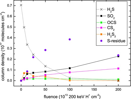
Column density of selected species as a function of ion fluence after irradiation of a CO:H2S = 10:1 ice mixture at 20 K, using the data from Garozzo et al. (2010). Solid and dotted lines have been drawn to guide the eye.
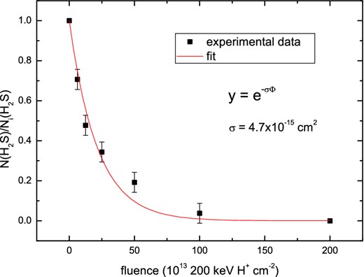
Column density ratio N(H2S)/Ni(H2S) of hydrogen sulphide as a function of ion fluence (Φ) after irradiation of the ice mixture. Data points are taken from Garozzo et al. (2010) and fitted with an exponential curve.
A list of the experimentally-detected sulphur-bearing species and their laboratory production cross-sections.
| Molecule | p (cm2) |
|---|---|
| H2S2 | 1.03 × 10⁻¹⁵ |
| SO2 | 6.78 × 10⁻¹⁶ |
| CS2 | 2.64 × 10⁻¹⁶ |
| OCS | 2.05 × 10⁻¹⁶ |
| S-residue | 1.19 × 10⁻¹⁵ |
| Molecule | p (cm2) |
|---|---|
| H2S2 | 1.03 × 10⁻¹⁵ |
| SO2 | 6.78 × 10⁻¹⁶ |
| CS2 | 2.64 × 10⁻¹⁶ |
| OCS | 2.05 × 10⁻¹⁶ |
| S-residue | 1.19 × 10⁻¹⁵ |
Three important considerations come from the analysis of the data taken from Garozzo et al. (2010).
A detection of CS2 has not yet been made in the ISM. Laboratory data allow us to quantify the abundance of this molecule and to extend our model to include a reaction scheme for its formation and loss channels.
- There is evidence of a residue of species containing sulphur, that can be estimated as follows:This residue provides a constant supply of sulphur and it may affect the role of sulphur as an evolutionary tracer. Moreover, as stated by Anderson et al. (2013), the sputtering of this residue from the surface could lead to the release of the large amount of atomic sulphur seen in shock regions.(1)\begin{eqnarray} N({\rm S{-}residue}) &=& N_{i}(\mathrm{H_{2}S})-N(\mathrm{H_{2}S})-N(\mathrm{SO_{2}}) -N(\mathrm{OCS}) \nonumber\\ &&-\,2N(\mathrm{CS_{2}})-2N(\mathrm{H_{2}S_{2}}). \end{eqnarray}
These experiments help to predict the different forms that sulphur can take on the grain surface and to estimate the ratios among sulphur-bearing molecules.
We therefore insert into ucl_chem the chemical reactions experimentally investigated by Garozzo et al. (2010) and reported in Table 3. Note that the reactions listed in Table 3 are simplified representations of a complex experimental process. The action of the high-energy protons on the laboratory ice analogues causes ∼105 molecular bonds to break, leading to a chain of recombination reactions. As a result of these very rapid recombinations, the products on the right-hand side are observed. These reactions do not take place in thermodynamic equilibrium. The remaining sulphur, or mSres, stays as a refractory element on the surface. The rate constants, k (s−1), have been evaluated by the product of the reaction cross-section (σ in cm2) and the flux of cosmic ions (FISM in cm−2 s−1). To apply the laboratory results to ISM conditions both quantities have been corrected using the following assumptions:
We derive the flux of cosmic ions in the approximation of effectively mono-energetic 1 MeV protons (Mennella et al. 2003): FISM = 0.22 ions cm−2 s−1. FISM must be regarded as an effective quantity: it represents the equivalent flux of 1 MeV protons which gives rise to the ionization rate produced by the cosmic ray spectrum if 1 MeV protons were the only source for ionization.
Furthermore, we speculate that the cross-section scales with the stopping power (SP, the energy loss per unit path length of impinging ions). According to the srim code by Ziegler & Biersack (2009), in the case of protons impinging on a CO:H2S mixture, SP(200 keV protons) = 2.7× SP(1 MeV protons).
Dissociation of solid H2S due to cosmic ray impact (CR) experimentally investigated by Garozzo et al. (2010). All the reaction channels are provided with a rate (in s−1) of ISM relevance. The m before the molecular formula stands for mantle.
| Reaction | k = α (s−1) |
|---|---|
| mH2S + CR|$_{\phantom{1}}$| → mSres + H2 | 9.53 × 10⁻¹⁷ |
| mH2S + mCO|$_{\phantom{1}}$| → mOCS + H2 | 1.65 × 10⁻¹⁷ |
| mH2S + mH2S → mH2S2 + H2 | 8.23 × 10⁻¹⁷ |
| 2mH2S + mCO|$_{\phantom{1}}$| → mCS2 + mO + 2H2 | 2.12 × 10⁻¹⁷ |
| mH2S + 2mO|$_{\phantom{1}}$|→ mSO2 + H2 | 5.42 × 10⁻¹⁷ |
In the case of hydrogen sulphide we define σISM = σ/2.7 cm2 and we derive a destruction rate of hydrogen sulphide equal to 3.8 × 10⁻¹⁶ s−1. In the case of species formed after irradiation we define σISM = p/2.7 cm2 (see Table 2 for p values) and the calculated formation rates for each species are given in Table 3.
In our code, two-body grain-surface reactions are considered to be bimolecular reactions occurring as they would in the gas phase, meaning that the parameter α should be expressed in units of volume (cm3 s−1). Since the data from experiments are in units of time, we have followed a procedure (see Occhiogrosso et al. 2011) for evaluating the rate coefficients for the formation of S-bearing species in the icy mantle, viz-à-viz, we consider an excess of one of the reactants. The rate of the reaction will therefore vary only with the concentration of the second reactant. As the total amount of ice varies with time, we calculate a value for the rate of each reaction that varies with time. For instance, when we consider CO as the most abundant reactant (this is the case of the second and the fourth reaction in Table 3), reaction rates cover six orders of magnitude because of the wide range spanned by the CO abundances during the collapse phase of protostar formation. We point out that density and freeze-out rate indeed play a pivotal role in controlling the trends of the molecular abundances and since both of these two physical parameters only significantly change towards the end of the collapse, we therefore refer only to the final abundance of CO in order to scale our reaction rates.
3.1.2 Laboratory investigations of solid OCS formation
3.2 Incorporation of new theoretical data into the model
In order to investigate the form of sulphur once it freezes on to the grain surface, we insert an extended chemistry including all the S-bearing species mentioned in the previous subsection into our gas–grain chemical network. In addition to these reactions, we also insert two new paths for the formation of carbonyl sulphide, OCS, as theoretically investigated by Adriaens et al. (2010). Reactions are listed in Table 4. The rate parameters relative to each channel are also reported; γ represents the reaction barrier in units of kelvin (K). Note that, unlike Adriaens et al. (2010), we do not account for the formation of any adduct species and we do not distinguish among the cis-trans geometries of the reactants and the products. The adsorption energies calculated by Adriaens et al. (2010) were smaller in value than those experimentally determined in previous studies (Mattera et al. 1980; Piper, Morrison & Peters 1984) due to the fact that the theory considers a perfect coronene surface and neglects the weak physisorption interactions observable in the presence of substrate defects. Every reaction activation barrier given can therefore be seen as an upper limit to the effective barrier.
Routes to OCS formation on a coronene surface, from Adriaens et al. (2010). α, β, γ represent the parameters for the rate coefficient in the modified Arrhenius equation. They have been adapted for a water-ice surface by Adriaens (private communication).
| Reaction | α (s−1) | β | γ (K) |
|---|---|---|---|
| CO + S → OCS | 1.66 × 10⁻¹¹ | 0 | 1893 |
| CO + HS → OCS + H | 1.66 × 10⁻¹¹ | 0 | 831 |
| Reaction | α (s−1) | β | γ (K) |
|---|---|---|---|
| CO + S → OCS | 1.66 × 10⁻¹¹ | 0 | 1893 |
| CO + HS → OCS + H | 1.66 × 10⁻¹¹ | 0 | 831 |
In addition to incorporating a grain-surface reaction network for sulphur-bearing species as a revision to the original version of the code, we also update our gas-phase reaction network with new rate coefficients taken from the KIDA data base (Wakelam et al. 2012). In particular, we insert or amend the rate parameters from the UMIST data base for different OCS routes of formation as described in Loison et al. (2012, see Table 5).
Gas-phase paths of OCS formation and destruction and their competitive routes. The revised α values are taken from Loison et al. (2012).
| Reaction | New α values | Previous α values |
|---|---|---|
| (cm3 mol−1 s−1) | (cm3 mol−1 s−1) | |
| CH + SO → OCS + H | 1.1 × 10⁻¹⁰ | – |
| CH + SO → SH + CO | 9.0 × 10⁻¹¹ | – |
| O + HCS → OCS + H | 5.0 × 10⁻¹¹ | 5.0 × 10⁻¹¹ |
| O + HCS → SH + CO | 5.0 × 10⁻¹¹ | – |
| H + HCS → H2 + CS | 1.5 × 10⁻¹⁰ | 4.0 × 10⁻⁹ |
| S + HCO → OCS + H | 8.0 × 10⁻¹¹ | – |
| S + HCO → SH + CO | 4.0 × 10⁻¹¹ | 3.6 × 10⁻¹⁰ |
| OH + CS → OCS + H | 1.7 × 10⁻¹⁰ | 9.4 × 10⁻¹⁴ |
| OH + CS → SH + CO | 3.0 × 10⁻¹¹ | – |
| C + OCS → CO + CS | 1.0 × 10⁻¹⁰ | 1.6 × 10⁻⁹ |
| CH + OCS → CO + CS + H | 4.0 × 10⁻¹⁰ | – |
| CN + OCS → CO + NCS | 1.0 × 10⁻¹⁰ | – |
4 PRESENTATION OF RESULTS
4.1 Trends among the data
We commence by setting the initial fractional abundance of gaseous sulphur ions equal to 1.4 × 10⁻⁶ (as measured by Sofia, Cardelli & Savage 1994). We also fix the physical parameters to values typical of high-mass SFRs, listed in Table 6.
Physical parameters for the model of a prototypical high-mass star. fr gives an indication of the freeze-out efficiency, maxt is the maximum temperature reached in the model, size is the diameter of the hot core, dens (df) is the (maximum) density reached in the collapse, at a time earlier than tfin. ζ represents the cosmic ray ionization rate.
| Parameter | Value |
|---|---|
| temp (K) | 10 |
| fr (per cent) | 98 |
| maxt (K) | 100 |
| size (pc) | 0.03 |
| dens (cm−3) | 2 × 10² |
| df (cm−3) | 1 × 10⁷ |
| tfin (yr) | 1 × 10⁷ |
| ζ (s−1) | 1.3 × 10⁻¹⁷ |
| Parameter | Value |
|---|---|
| temp (K) | 10 |
| fr (per cent) | 98 |
| maxt (K) | 100 |
| size (pc) | 0.03 |
| dens (cm−3) | 2 × 10² |
| df (cm−3) | 1 × 10⁷ |
| tfin (yr) | 1 × 10⁷ |
| ζ (s−1) | 1.3 × 10⁻¹⁷ |
Since we aim to investigate the effect of the new surface reactions on the abundances of the S-bearing species, we have to allow molecules to freeze on to the grain. In particular, we consider two limiting cases where each species freezes as itself (F1) or it hydrogenates (F2) and an intermediate case (F3) where we hydrogenate half of the accreting S-bearing species. The grid of the freeze-out pathways chosen is reported in Table 7. Note that not all the sulphur-bearing species included in our model are shown; in particular, we assume that H2S, H2CS, OCS, SO2, NS, SO, CS2 and H2S2 accrete on to the grains without hydrogenating.
Grid of possible paths of freeze-out for S-bearing molecules.
| Model | S→grains | HS→grains | HS2→grains | S2→grains | CS→grains | HCS→grains |
|---|---|---|---|---|---|---|
| 100 per cent mS | 100 per cent mHS | 100 per cent mHS2 | 100 per cent mS2 | 100 per cent mCS|$_{\phantom{2}}$| | 100 per cent mHCS|$_{\phantom{2}}$| | |
| F1 | ||||||
| 0 per cent mH2S | 0 per cent mH2S | 0 per cent mH2S2 | 0 per cent mH2S|$_{\phantom{2}}$| | 0 per cent mHCS | 0 per cent mH2CS | |
| 0 per cent mS | 0 per cent mHS | 0 per cent mHS2 | 0 per cent mS2 | 0 per cent mCS|$_{\phantom{2}}$| | 0 per cent mHCS|$_{\phantom{2}}$| | |
| F2 | ||||||
| 100 per cent mH2S | 100 per cent mH2S | 100 per cent mH2S2 | 100 per cent mH2S|$_{\phantom{2}}$| | 100 per cent mHCS | 100 per cent mH2CS | |
| 50 per cent mS | 50 per cent mHS | 50 per cent mHS2 | 50 per cent mS2 | 50 per cent mCS|$_{\phantom{2}}$| | 50 per cent mHCS|$_{\phantom{2}}$| | |
| F3 | ||||||
| 50 per cent mH2S | 50 per cent mH2S | 50 per cent mH2S2 | 50 per cent mH2S|$_{\phantom{2}}$| | 50 per cent mHCS | 50 per cent mH2CS |
In addition, we need to derive an estimate of the sulphur species in the gas phase, after their thermal evaporation from the grain surface, for comparison to evolved hot cores. As investigated by Viti et al. (2004), species can evaporate from the icy mantle in different bands of temperatures; in particular, Viti et al. (2004) determined that H2CS behaves as an H2O-like molecule that codesorbs with the H2O-ice when it starts to sublime from the grain surface (at ∼100 K). Moreover, the authors classified HCS, OCS, H2S, SO2 as intermediate species since they showed two peaks (due to volcano and codesorption effects) in their Temperature Programmed Desorption traces. After further discussion (Brown, private communication), we have revised the above desorption classification (Viti et al. 2004) as follows:
HS, H2S2, OCS, H2S, SO2, HCS, NS as intermediate
H2CS, SO as water-like
HS2 as reactive
S2, CS2, S-residue as refractory.
No sulphur-bearing species are classified as having a desorption behaviour that is CO-like (the initial desorption category of Viti et al. 2004).
In order to assess the impact of our updates on the chemical network, we ran some test models, comparing our original version of the code and those including the new sets of reactions. Our findings are reported in Table 8. The changes in the ice composition are more evident at the end of the collapse phase (Phase I), when temperatures are as low as 10 K. Note that we only show our results assuming the highest degree of hydrogenation (F2) during the freeze-out of the molecules, and we reserve a more detailed investigation for later in the paper.
Fractional abundances (with respect to H2) of solid sulphur-bearing species obtained as outputs from our code before (OLD) and after (NEW) our updates at the end of Phase I. The m before the molecular formula stands for mantle.
| Species | OLD | NEW |
|---|---|---|
| mCS | 2.6 × 10⁻¹³ | 2.6 × 10⁻¹³ |
| mOCS | 3.9 × 10−09 | 6.6 × 10−09 |
| mHCS | 1.6 × 10−08 | 1.8 × 10−08 |
| mH2S | 1.4 × 10−06 | 1.4 × 10−06 |
| mH2CS | 5.8 × 10−09 | 5.7 × 10−09 |
| mS | Trace | Trace |
| mS2 | 5.8 × 10⁻¹³ | 2.4 × 10⁻¹³ |
| mSO | 8.8 × 10⁻¹⁰ | 9.2 × 10⁻¹⁰ |
| mSO2 | 5.4 × 10⁻¹⁰ | 5.7 × 10⁻¹⁰ |
| mNS | 9.9 × 10⁻¹² | 1.1 × 10⁻¹¹ |
| mHS | Trace | Trace |
| mHS2 | 3.2 × 10⁻¹⁴ | 3.7 × 10⁻¹³ |
| mH2S2 | 1.1 × 10⁻¹² | 2.2 × 10⁻¹⁰ |
| mCS2 | None | 8.7 × 10⁻¹⁵ |
| mS-residue | None | 5.4 × 10−09 |
Scrutinizing Table 8, we immediately observe that the most abundant sulphur species in the solid state is H2S, which is predictable since we are discussing the model with the highest degree of hydrogenation. The abundance of OCS is enhanced in the new model by a factor of ∼2; this is mostly due to the reaction of H2S + CO on the grain surface, with the rate from Garozzo et al. (2010). The reaction studied by Ward et al. (2012) contributes at the level of a few per cent. The most interesting result is definitely the amount of sulphur residue (S-residue) that we are now able to produce on the grain. As we can see, in the updated version of the code, S-residue is in fact the fifth most abundant ice-mantle S-bearing species. These findings are extremely important, both because they match what has been already experimentally determined by Jiménez-Escobar et al. (2014) as an attempt to explain the lack of sulphur in dense regions. We now need to provide a better estimate of this residue in order to understand how its presence might affect the total amount of interstellar sulphur; we have decided not to speculate more about its nature, since only experiments can give us information on the chemical structure of these refractory molecules, but refer the interested reader to Steudel (2003).
Based on the computational work that has previously been performed in this area (see Introduction) as well as on some simple test models, we have not investigated changes in the temperature or in the density of our sources; instead, we analyse how the calculated abundances vary with the cosmic ray ionization rate by choosing a standard interstellar (ζ0 = 1.3 × 10⁻¹⁷ s−1), an enhanced (1.3 × 10⁻¹⁶ s−1) and a super-enhanced (1.3 × 10⁻¹⁵ s−1) value for this parameter. With these parameters we then repeat our sensitivity tests for each freeze-out chemistry (F1, F2, F3; Table 7). Figs 3 and 4 display the most abundant species found at the end of the collapse phase (where temperatures are as low as 10 K and only non-thermal desorption can occur) and when the hot core is finally formed (≥100 K), respectively. Note that while Fig. 3 shows the different molecules in the solid state (on the grain surface), in Fig. 4 we report the species in the gas phase, with the exception of the S-residue. Both figures show the phase where the bulk sulphur is located, and despite the increase in ζ, cosmic ray induced desorption in not efficient enough in our models to return a significant amount of sulphur to the gas phase in Phase I. Specifically, in models with ζ = ζ0, we find about 0.02 per cent of sulphur in the gas phase. In models with ζ = 100ζ0, this percentage rises to ∼0.5 per cent of the elemental sulphur in the gas phase at the end of Phase I.
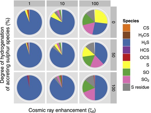
The most abundant S-bearing species in the icy mantle at the end of the collapse phase (Phase I). 0, 50 and 100 on the vertical axis refer to the percentage of hydrogenation chosen (see text); 1, 10, 100 indicate a standard, an enhanced and a super-enhanced cosmic ionization rate, respectively.
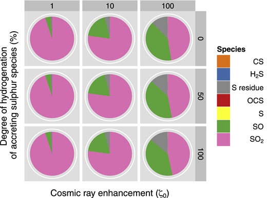
The most abundant S-bearing species in the gas (excluding the residue, which is solid) at the end of the desorption phase (Phase II). 0, 50 and 100 on the vertical axis refer to the percentage of hydrogenation chosen (see text and Table 7); 1, 10, 100 indicate a standard, an enhanced and a super-enhanced cosmic ray ionization rate, respectively.
Phase I appears to be dominated by H2S (in agreement with the scheme of Hatchell et al. 1998), where the abundance seems to be influenced by the degree of ionization as well as by the percentage of hydrogenation. Starting the discussion of trends in the results by considering the case with 0 per cent hydrogenation (top panels), going from left to the right in Fig. 3, the increase in the ζ values (from the standard to the super-enhanced) leads to a more efficient non-thermal desorption of H2S, which therefore decreases in the icy mantle in favour of other S-bearing species. The immediate consequence is a greater amount of hydrogen sulphide in the gas phase. The latter species then reacts with atomic ions (C+, S+, H+) at early times and molecular ions (H3O+, HCO+) at late times to liberate atomic sulphur, which goes on to react with OH in order to produce SO and SO2. These oxides are then frozen back on to the grain. Moreover, we highlight a predictable increase in the S-residue abundance (since the rate of cosmic ray ionization directly depends on the ζ value) and an increasingly inefficient formation of solid OCS, which is mainly produced on the grain by reaction between H2S and CO. Moving to the bottom panels, the chemical behaviour is altered by the higher level of hydrogenation. At the beginning the situation is very similar to the one described above, but once gaseous HS and S are formed, they will both freeze back on to the grain as H2S. Therefore, assuming a super-enhanced cosmic ray ionization rate, compared to the previous case, we now observe a larger amount of H2S, OCS and S-residue in the solid state.
Phase II is dominated by SO2 and the second most abundant species is SO. This result is not surprising. If we look at the chain of reactions mentioned above, we actually find that gaseous H2S, S and HS will eventually lead to the formation of SO and SO2. The chemistries of these two species are strongly related to each other: SO forms SO2 by reaction with O or OH; SO2 produces SO when reacting with C. We notice immediately from Fig. 4 that the SO/SO2 ratio is sensitive to the cosmic ray ionization field, increasing with field strength. Finally, as we can see in Fig. 4, an observable abundance of S-residue is still locked inside the grain, even after the ice mantle has been completely desorbed.
4.2 Comparison of theoretical results with recent observations
In order to verify the reliability of our calculations, we looked at the observed abundances of 21 species in hot cores and high-mass SFRs reported in the literature in the last five years. The reader should bear in mind that when performing a comparison such as this, order of magnitude agreement between observation and model results is excellent. Telescope beams often cover large regions, resulting in average column densities and abundances (averaged over both temperature and density variations), and since it is observationally very hard to determine the evolutionary stage of a hot core, it becomes equally hard to identify a ‘t = 0’ to which to anchor the model results. Despite these caveats, a comparison between observational and model results is an important check of the model.
Herpin et al. (2009) surveyed four hot cores using the IRAM 30 m and CSO telescopes, and detected lines of CS, OCS, H2S, SO, SO2 and their 34S isotopologues. Qin et al. (2010) used the SMA interferometer to observe G19.61-0.23, detecting 17 molecules, including SO, SO2, OCS and CS and various isotopologues. Of these four molecules, only the SO abundance was determined using more than one line. Neufeld et al. (2012) discovered the mercapto radical (HS) in the high-mass SFR, W49N, and also provided a measurement of the H2S abundance there. Zernickel et al. (2012) performed a sub-mm survey of the high-mass SFR NGC 6334I, detecting over 20 molecules in two hot cores. Several of these molecules are sulphur-bearing: OCS, CS, SO, H2S, SO2 and H2CS. Xu & Wang (2013) also used the SMA interferometer to observe a massive SFR, G20.080.14N, detecting 11 molecular species, including SO and SO2. Finally, Gerner et al. (2014) observed a large sample of 59 high-mass SFRs at various stages of evolution, including 11 hot molecular cores. 16 molecules were detected, of which four – 13CS, SO, C33S, OCS – contain sulphur. Note that all these cores span a range of masses, distances and evolutionary stages.
We compared fractional abundances calculated by our models at 105 yr of Phase II, for three values of the cosmic ray ionization rate in Fig. 5. Variations in hydrogenation efficiency during Phase I have little effect on the gas-phase abundances in Phase II, and thus we present results from ‘50 per cent hydrogenation’ models only. In general, the agreement between calculated abundances and abundances derived from the observations is very good: models and observational results are in agreement for two-thirds of the species, and in the some of the remaining third, disagreement is less than an order of magnitude. There are issues with species which are formed mostly by UV and CR dissociation: CN, N2H+, C2H and HCO+ are underestimated by our model. In the model, interstellar UV photons are assumed to become extinguished in the outer core material. Only cosmic ray induced UV photons play an active part in the chemistry of our simulations. Hot cores, in reality, may be significantly fragmented, allowing UV photons to penetrate more deeply into the core than in a homogeneous medium. This may account for our underestimation of these species in our model. There is little evidence in our galaxy for cosmic ray ionization rates higher than those tested in our model (Dalgarno 2006).
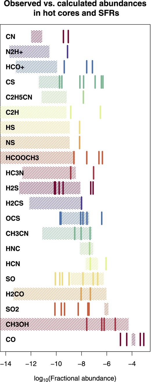
Observed (solid coloured lines) and ranges of calculated abundances from our models (hatched regions) for the species reported in a number of recent observational papers (Herpin et al. 2009; Qin et al. 2010; Neufeld et al. 2012; Zernickel et al. 2012; Xu & Wang 2013; Gerner et al. 2014), dealing with hot cores and high-mass SFRs.
Observations indicate that CS is the most abundant sulphur-bearing species; however, models struggle to produce enough CS to match observed amounts. This is a recurrent problem in warm-temperature chemical models (e.g. Wakelam et al. 2011). This underestimation may stem from a lack of understanding of the warm-temperature chemistry of CS, incorrect rate coefficients for its gas-phase reactions, shock passage through the observed regions (Viti et al. 2001), etc. Other sulphur-bearing species are observed to have similar abundances to each other: OCS, H2S, SO, SO2, H2CS and HS, all have average fractional abundances in the range 7–70 × 10−9 in Fig. 5. Simulation results are within the same range for all the above species with the exception of SO2, which seems to be overestimated, and SO, which appears to be underproduced (the relationship between these two species has already been discussed in detail – see Section 4.1).
In Table 9, we present the abundances of sulphur-bearing species for three values of ζ, the cosmic ray ionization rate. Note that we also include the abundances of species which have not been observed to date and the amount of a potential residue. No ions are shown, since they are of low abundance (x(ion)≤10−14), and do not contribute significantly to the sulphur budget. As previously mentioned, apart from CS and SO2, agreement is good between calculated abundances of sulphur-bearing species and their observed values. An interesting finding is that the abundance of H2S2 reaches observable levels; therefore, the absence of its detection to date might be only due to the fact that this molecule has a small dipole moment (∼1.2 D).
Calculated fractional abundances of selected sulphur-bearing species as a function of cosmic ray ionization rate, compared to their mean observed values towards various hot cores. Data are taken from Herpin et al. (2009), Qin et al. (2010), Neufeld et al. (2012), Zernickel et al. (2012), Xu & Wang (2013) and Gerner et al. (2014).
| Species | Standard model | Enhanced model | Super-enhanced model | Observed range |
|---|---|---|---|---|
| SO2 | 1.3 × 10⁻⁶ | 1.3 × 10⁻⁶ | 7.2 × 10⁻⁷ | 7.9 × 10⁻¹¹–3.9 × 10⁻⁸ |
| SO | 4.9 × 10⁻⁹ | 1.5 × 10⁻⁹ | 6.1 × 10⁻⁷ | 8.5 × 10⁻¹¹–1.9 × 10⁻⁷ |
| OCS | 2.9 × 10⁻⁸ | 5.5 × 10⁻⁹ | 2.6 × 10⁻¹⁰ | 2.0 × 10⁻¹⁰–4.0 × 10⁻⁷ |
| H2CS | 1.1 × 10⁻⁸ | 3.9 × 10⁻⁹ | Trace | 1.0 × 10⁻⁸ |
| H2S | 8.5 × 10⁻⁹ | Trace | 1.0 × 10⁻¹² | 7.3 × 10⁻¹¹–8.3 × 10⁻⁸ |
| CS | 1.0 × 10⁻¹⁰ | 4.1 × 10⁻¹² | 3.1 × 10⁻¹⁰ | 1.8 × 10⁻¹⁰–5.0 × 10⁻⁷ |
| HS | 1.2 × 10⁻⁹ | Trace | Trace | 7.0 × 10⁻⁹ |
| NS | 1.2 × 10⁻⁹ | Trace | Trace | 4.2 × 10⁻⁹ |
| HCS | 5.5 × 10⁻¹¹ | Trace | Trace | – |
| S | 3.2 × 10⁻¹¹ | 1.9 × 10⁻¹¹ | 3.5 × 10⁻¹⁰ | – |
| HS2 | 4.0 × 10⁻¹⁰ | 2.3 × 10⁻¹⁰ | Trace | – |
| H2S2 | 1.7 × 10⁻⁹ | 6.8 × 10⁻¹⁰ | Trace | – |
| S2 | 2.4 × 10⁻⁹ | Trace | Trace | – |
| mS2 | Trace | 1.5 × 10⁻¹² | 7.9 × 10⁻¹² | – |
| mCS2 | Trace | Trace | Trace | – |
| S-residue | 5.5 × 10⁻⁹ | 2.3 × 10⁻⁸ | 8.5 × 10⁻⁸ | – |
From Table 9, it is evident that the abundances of most sulphur-bearing species are influenced by ζ, with some molecules only being significantly present in standard ζ environments (HS, NS, HCS). In order to make these changes more evident, we plot the fractional abundance of the S-bearing species as a function of the time during the desorption phase (Fig. 6). In addition, we show the variation of H2O, HNC and CO, as standards for our models. In general, abundant molecules, such as SO and OCS, are present at observational levels at all three strengths of ζ and may be good tracers of ζ if their observed abundances can be tightly constrained. SO2 is also abundant at high levels throughout the tests, but does not vary much in abundance.
![Results from the warm-up phase of the model, showing the effect of the cosmic ray ionization rate upon the fractional abundances of various species. The left-hand panel is extended slightly to show the desorption events [those of the (i) pure species on the surface of the ice, (ii) monolayer on H2O ice, (iii) volcano desorption and (iv) codesorption with H2O. See Viti et al. 2004, for a full description]. The right-hand panel shows species labels. This figure highlights the issues with comparing model results at a certain time to observational values, since fractional abundances can vary by several orders of magnitude.](https://oup.silverchair-cdn.com/oup/backfile/Content_public/Journal/mnras/450/2/10.1093/mnras/stv652/2/m_stv652fig6.jpeg?Expires=1716456529&Signature=V4QGA-I2jCmQE16psMMTrXUWuSKQeKuX9Gn5BXt5Dlh74tMVyjlPLJzvkRFVPdKNx9A66HBHxCuBnpFCoPQPV6ko9PL5gRSnCuk1bkEWAys36hUIAQ9N3Y2qUTMm0Rkatjwr~Nq5neE47MVls5MbNfpRWpqxZLpeKdM2fb4R5S5XEKIgPw1Nr7sKt-oqsxlsZtXF~RpQ3FPEawMiZjQAEyBQK1r06sfjcV7f6E1yFeUO58~24-d31bPHBFRquRkkr-axYY0TXN-Y4bhnX5hPyY1kunD16XmuhOo7gWcHGZFvi2xBM0GOaqydRjracDIU8lj1Bi-WIv6JM~b8LAkrQQ__&Key-Pair-Id=APKAIE5G5CRDK6RD3PGA)
Results from the warm-up phase of the model, showing the effect of the cosmic ray ionization rate upon the fractional abundances of various species. The left-hand panel is extended slightly to show the desorption events [those of the (i) pure species on the surface of the ice, (ii) monolayer on H2O ice, (iii) volcano desorption and (iv) codesorption with H2O. See Viti et al. 2004, for a full description]. The right-hand panel shows species labels. This figure highlights the issues with comparing model results at a certain time to observational values, since fractional abundances can vary by several orders of magnitude.
A further consideration evident in Fig. 6 is that the abundances of some species vary considerably with time, and as stated in the introduction to this section, this makes comparisons with observations challenging. For instance, gas-phase H2S abundances drop in all scenarios by almost six orders of magnitude, but on different time-scales, and H2CS abundances by almost four orders of magnitude. Other species vary in abundance by an order of magnitude or so, whereas species like SO2 are present at their solid-phase abundances, i.e. their abundances are unaltered by gas-phase chemistry.
If we now consider the refractory sulphur-bearing species, S2, CS2 and the sulphur residue, it is evident that an appreciable amount (up to 6 per cent) of sulphur in our model is locked in form of this residue. It is hard to speculate about the chemical nature of this residue; recent experiments (Jiménez-Escobar et al. 2014) seem to attribute its existence to the formation of sulphur polymers, such as S8. There may, of course, be several ways to sink sulphur into this refractory residue, and we only consider a single route here, led by the experimental evidence.
Finally, we are able to produce detectable abundances of species such as H2S and CS but only on the grain surface (Table 8). This means that, while there is a good understanding of the mantle sulphur chemistry, the rates of some gas-phase reactions need to be refined; in particular, the key step seems to be the high efficiency of SO and SO2 formation from S and HS as reactants.
5 CONCLUSIONS
In summary, we have extended the ucl_chem chemical model to include new experimental and theoretical results on sulphur chemistry; in particular, we have inserted laboratory data from experiments where H2S ice is processed by protons which simulate cosmic ray impacts on the grain surface. Garozzo et al. (2010) detected in their icy mantle analogues the formation of CS2, which has not been observationally detected in the gas-phase ISM yet. In our modelling, we find that CS2 was only present in small amounts in icy mantles. Following on from the experiment by Garozzo et al. (2010), Ward et al. (2012) studied the production of solid OCS from CS2 and O ice. We therefore also added the latter reaction to our chemical network. OCS abundances were enhanced by a factor of ∼2, driven mainly by the Garozzo et al. (2010) reaction, mH2S + mCO |$\longrightarrow$| mOCS + H2, and only partially by the reaction from Ward et al. (2012). Finally, we also revised our gas-phase reactions based on recent papers by Loison et al. (2012) and Adriaens et al. (2010). We looked at the influence of the new reaction network on the fractional abundances of selected S-bearing species by comparing the results with the original version of our code. Abundances of species such as HS2 and H2S2 increased by large factors in the solid phase via very efficient hydrogenation of accreting species, but not significantly enough to make them major carriers of sulphur. Our main result was that a residue, left on the grain surface after ice desorption, could harbour a large amount of sulphur (10−8), in line with recent experiments (Jiménez-Escobar et al. 2014).
A comparison with astronomical observations was also carried out. Good agreement is obtained although we find it difficult to reconcile theoretical estimates with observations of some of the most abundant species such as H2S, CS and OCS. Our results show that at early stages during the collapse phase of star formation, H2S is the predominant sulphur-bearing species in the icy mantles. As the evolution of a pre-stellar core continues SO2 and SO are efficiently formed, in agreement with earlier work. In this respect, the pivotal processes appear to be the gas-phase production of SO and SO2 from S and HS as reactants. Another key factor to be considered is the presence of a sulphur residue on the grain surface, which may affect the observability of some species in the gas phase. This paper is therefore an important step forward in understanding the sulphur chemistry in regions of star formation as we constrain the problem to two main factors: the gaseous interactions between S or HS and O or OH to form SO and SO2 and the existence of a sulphur residue on the grain surface.
The research leading to these results has received funding from the (European Union's) Seventh Framework Program [FP7/2007-2013] under grant agreement no. 238258. This work was partly supported by the Italian Ministero dell'Istruzione, Università e Ricerca (MIUR) through the grant Progetti Premiali 2012 - iALMA. The research of ZK has been supported by VEGA – The Slovack Agency for Science, grant no. 2/0032/14.
