


Abstract
We report Hubble Space Telescope optical to near-infrared transmission spectroscopy of the hot-Jupiter WASP-6b, measured with the Space Telescope Imaging Spectrograph and Spitzer's InfraRed Array Camera. The resulting spectrum covers the range 0.29–4.5 μm. We find evidence for modest stellar activity of WASP-6 and take it into account in the transmission spectrum. The overall main characteristic of the spectrum is an increasing radius as a function of decreasing wavelength corresponding to a change of Δ (Rp / R*) = 0.0071 from 0.33 to 4.5 μm. The spectrum suggests an effective extinction cross-section with a power law of index consistent with Rayleigh scattering, with temperatures of 973 ± 144 K at the planetary terminator. We compare the transmission spectrum with hot-Jupiter atmospheric models including condensate-free and aerosol-dominated models incorporating Mie theory. While none of the clear-atmosphere models is found to be in good agreement with the data, we find that the complete spectrum can be described by models that include significant opacity from aerosols including Fe-poor Mg2SiO4, MgSiO3, KCl and Na2S dust condensates. WASP-6b is the second planet after HD 189733b which has equilibrium temperatures near ∼1200 K and shows prominent atmospheric scattering in the optical.
1 INTRODUCTION
Multiwavelength transit observations of hot Jupiters provide a unique window to the chemistry and structure of the atmospheres of these distant alien worlds. During planetary transits, a small fraction of the stellar light is transmitted through the planetary atmosphere and signatures of atmospheric constituents are imprinted on the stellar spectrum (Seager & Sasselov 2000). Transmission spectroscopy, where the planet radius is measured as a function of wavelength, has revolutionized our understanding of extrasolar gas-giant atmospheres. Numerous studies from both space- and ground-based observations have led to the characterization and detection of atomic and molecular features as well as hazes and clouds in the atmospheres of several hot Jupiters revealing a huge diversity (Charbonneau et al. 2002; Grillmair et al. 2008; Pont et al. 2008, 2013; Redfield et al. 2008; Snellen et al. 2008, 2010; Sing et al. 2011, 2012, 2013; Brogi et al. 2012; Bean et al. 2013; Birkby et al. 2013; Deming et al. 2013; Gibson et al. 2013a,b; Huitson et al. 2013; Wakeford et al. 2013; Nikolov et al. 2014; Stevenson et al. 2014).
Atmospheric hazes have currently been detected in hot-Jupiter exoplanets over a wide range of atmospheric temperature regimes including HD 189733b and WASP-12b representing the cool and hot extremes for hot Jupiters at equilibrium temperatures around 1200 and 3000 K, respectively. Hazes are considered to originate from dust condensation (forming aerosols in the atmospheres of exoplanets) or a result from photochemistry (Marley et al. 2013). Transmission spectroscopy studies may constrain the most probable condensates responsible for these two planets, with iron-free silicates (e.g. MgSiO3) and corundum (Al2O3) being two prime candidates for the above temperature regimes (Lecavelier Des Etangs et al. 2008a; Sing et al. 2013). Cloud-free hot-Jupiter atmospheric models predict sodium and potassium to be the dominant absorbing features in optical transmission spectra (Seager & Sasselov 2000; Fortney et al. 2005).
In this paper, we present new results for WASP-6b from a large Hubble Space Telescope (HST) hot-Jupiter transmission spectral survey comprising eight transiting planets. The ultimate aim of the project is to explore the variety of hot-Jupiter atmospheres, i.e. clear/hazy/cloudy, delve into the presence/lack of TiO/alkali and other molecular features, probe the diversities between possible sub-classes and perform comparative exoplanetology. Initial results from four exoplanets have been presented so far in Huitson et al. (2013) for WASP-19b, Wakeford et al. (2013) and Nikolov et al. (2013) for HAT-P-1b and Sing et al. (2013) for WASP-12b and Sing et al. (2015) for WASP-31b. Already a wide diversity among exoplanet atmospheres is observed. In this paper, we report new HST optical transit observations with the Space Telescope Imaging Spectrograph (STIS) instrument and combine them with Spitzer InfraRed Array Camera (IRAC) broad-band transit photometry to calculate a near-UV to near-infrared transmission spectrum, capable of detecting atmospheric constituents. We describe the observations in Section 2, present the light-curve analysis in Section 3, discuss the results in Section 4 and conclude in Section 5.
1.1 The WASP-6b system
Discovered by the Wide Angle Search for Planets, WASP-6 b is an inflated sub-Jupiter-mass transiting extrasolar planet orbiting a moderately bright V = 11.9 solar-type, mildly metal-poor star (with Teff = 5375 ± 65 K, log g = 4.61 ± 0.07 and [Fe/H]=−0.20 ± 0.09) located in the southern part of the constellation Aquarius (Gillon et al. 2009; Doyle et al. 2013). The planet is moving on an orbit with a period of P ≃ 3.6 d and semimajor axis a ≃ 0.042 au. The sky-projected angle between the stellar spin and the planetary orbital axis has been determined through observations of the Rossiter–McLaughlin effect by Gillon et al. (2009) indicating a good alignment (|${\rm {\beta =11^{+14}_{-18}\ deg}}$|) that consequently favours a planet migration scenario via the spin–orbit preserving tidal interactions with a protoplanetary disc. Dragomir et al. (2011) refined the WASP-6 system parameters and orbital ephemeris from a single ground-based transit observation finding good agreement between their results and the discovery paper. Although Gillon et al. (2009) claimed evidence for non-zero orbital eccentricity, an analysis with new radial velocity data from Husnoo et al. (2012) brought evidence for non-significant eccentricity. Finally, Doyle et al. (2013) refined the spectroscopic parameters of WASP-6b's host star.
A cloud-free hot-Jupiter theoretical transmission spectrum predicts strong optical absorbers, dominated by Na i and K i absorption lines and H2 Rayleigh scattering for a planetary system with the physical properties of WASP-6b, including an effective planetary temperature (assuming zero albedo and f = 1/4 heat redistribution) of 1194 K and surface gravity g ≃ 8 m s−2 (Fortney et al. 2008; Burrows et al. 2010). The atmosphere of WASP-6b has recently been probed in the optical regime from the ground by Jordán et al. (2013). The authors found evidence for an atmospheric haze characterized by a decreasing apparent planetary size with wavelength and no evidence for the pressure-broadened alkali features.
2 OBSERVATIONS AND CALIBRATIONS
2.1 HST STIS spectroscopy
We acquired low-resolution (R = Δλ/λ = 500–1040) HST STIS spectra (Proposal ID GO-12473, P.I., D. Sing) during three transits of WASP-6 b on ut 2012 June 10 (visit 9) and 16 (visit 10) with grating G430L (∼2.7 Å pixel−1) and 2012 July 23 (visit 21) with grating G750L (∼4.9 Å pixel−1). When combined, the blue and red STIS data provide complete wavelength coverage from 2900 to 10 300 Å with a small overlap region between them from 5240 to 5700 Å (Fig. 1). Each visit consisted of five ∼96 min orbits, during which data collection was truncated with ∼45 min gaps due to Earth occultations. Incorporating wide 52 × 2 arcsec slit to minimize slit light losses and an integration time of 278 s, a total of 43 spectra were obtained during each visit. Data acquisition overheads were minimized by reading-out a reduced portion of the CCD with a size of 1024 × 128. This observing strategy has proven to provide high signal-to-noise ratio (S/N) spectra that are photometrically accurate near the Poisson limit during a transit event (Brown et al. 2001; Sing et al. 2011, 2013; Huitson et al. 2012). The three HST visits were scheduled such that the second and third spacecraft orbits occurred between the second and third contacts of the planetary transit in order to provide good sampling of the planetary radius while three orbits secured the stellar flux level before and after the transit.
Typical STIS G430L and G750L spectra (blue and red continuous lines, respectively). A fringe-corrected spectrum (offset by 5 × 10³ counts) is portrayed above the uncorrected red spectrum for comparison.
The data reduction and analysis process is somewhat uniform for the complete large HST programme and follows the general methodology detailed in Huitson et al. (2013), Sing et al. (2013) and Nikolov et al. (2014). The raw STIS data was reduced (bias-, dark- and flat-corrected) using the latest version of the CALSTIS1 pipeline and the relevant up-to-date calibration frames. Correction of the significant fringing effect was performed for the G750L data using contemporaneous fringe flat frame obtained at the end of the observing sequence and the procedure detailed in (Goudfrooij & Christensen 1998, Fig. 1).
Due to the relatively long STIS integration time (i.e. 287 s), the data contain large number of cosmic ray events, which were identified and removed following the procedures described in Nikolov et al. (2013). It was found that the total number of pixels affected by cosmic ray events comprise ∼4 per cent of the total number of pixels of each 2D spectrum. In addition, we also corrected all pixels identified by CALSTIS as ‘bad’ with the same procedure, which together with the cosmic ray identified pixels resulted in a total of ∼11 per cent interpolated pixels.
Spectral extractions were performed in iraf employing the APALL procedure using the calibrated .flt science files after fringe and cosmic ray correction. We performed spectral extraction with aperture sizes in the range 6.0–18.0 pixels with a step of 0.2. The best aperture for each grating was selected based on the resulting lowest light-curve residual scatter after fitting the white light curves (see Section 3 for details). We found that aperture sizes 12.0, 12.2 and 8.6 pixels satisfy this criterium for visits 9, 10 and 21, respectively. We then placed the extracted spectra to a common Doppler corrected rest frame through cross-correlation to prevent sub-pixel wavelength shifts in the dispersion direction. A wavelength solution was obtained from the x1d files from CALSTIS. The STIS spectra were then used to extract both white-light spectrophotometric time series and custom wavelength bands after integrating the appropriate flux from each bandpass.
The raw STIS light curves exhibit instrumental systematics similar to those described by Gilliland, Goudfrooij & Kimble (1999) and Brown et al. (2001). In summary, the major source of the systematics is related with the orbital motion of the telescope. In particular, the HST focus is known to experience quite noticeable variations on the spacecraft orbital time-scale, which are attributed to thermal contraction/expansion (often referred to as the ‘breathing effect’) as the spacecraft warms up during its orbital day and cools down during orbital night (Hasan & Bely 1993, 1994; Suchkov & Hershey 1998). We take into account the systematics associated with the telescope temperature variations in the transit light-curve fits by fitting a baseline function depending on various parameters (Section 3.0.1).
2.2 Spitzer IRAC data
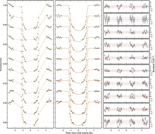
Photometric data were collected for WASP-6 during two transits of its planet on ut 2013 January 14 and 21 with the Spitzer space telescope (Werner et al. 2004) employing, respectively, the 4.5 and 3.6 μm channels of the IRAC (Fazio et al. 2004) as part of programme 90092 (P.I. J.-M. Desert). Both observations started shortly before ingress with effective integration times of 1.92 s per image and were terminated ∼2.2 h after egress resulting in 8 320 images (see Fig. 2), which were calibrated by the Spitzer pipeline (version S19.1.0) and are available in the form of Basic Calibrated Data (.bcd) files.
After organizing the data, we converted the images from flux in mega-Jansky per steradian (MJy sr−1) to photon counts (i.e. electrons) using the information provided in the fits headers. In particular, we multiplied the images by the gain and individual exposure time (fits header key words SAMPTIME and GAIN) and divided by the flux conversion factor (FLUXCONV). Timing of each image was computed using the UTC-based Barycentric Julian Date (BJDUTC) from the fits header key word BMJD_OBS, transforming these time stamps into BJD based on the BJD terrestrial time (TT) using the following conversion |$\rm {BJD_{TT}}\sim \rm {BJD_{UTC}}+ 66.184$| s (Eastman, Siverd & Gaudi 2010). This conversion is preferable as leap seconds are occasionally added to the BJDUTC standard (Knutson et al. 2012; Todorov et al. 2013).
We performed outlier filtering for hot (energetic) or lower pixels in the data by following each pixel through time. This task was performed in two steps, first flagging all pixels with intensity 8σ or more away from the median value computed from the five preceding and five following images. The values of these flagged pixels were replaced with the local median value. In the second pass, we flagged and replaced outliers above the 4σ level, following the same procedure. The total fraction of corrected pixels was 0.26 per cent for the 3.6 μm and 0.06 per cent for the 4.5 μm channel.
We estimated and subtracted the background flux from each image of the time series. To do this, we performed an iterative 3σ outlier clipping for each image to remove the pixels with values associated with the stellar point spread function (PSF), background stars or hot pixels, created a histogram from the remaining pixels and fitted a Gaussian to determine the sky background.
We measured the position of the star on the detector in each image incorporating the flux-weighted centroiding method2 using the background-subtracted pixels from each image for a circular region with radius 3 pixels centred on the approximate position of the star. While we could perform PSF centroiding using alternative methods such as fitting a two-dimensional Gaussian function to the stellar image, previous experiences with warm Spitzer photometry showed that the flux-weighted centroiding method is either equivalent or superior (Beerer et al. 2011; Knutson et al. 2012; Lewis et al. 2013). The variation of the x and y positions of the PSF on the detectors were measured to be 0.20 and 0.21 for the 3.6 μm channel and 0.89 and 0.8 pixels for the 4.5 μm channel.
We extract photometric measurements from our data following two methods. First, aperture photometry was performed with idl routine APER using circular apertures ranging in radius from 1.5 to 3.5 pixels in increments of 0.1. We filtered the resulting light curves for 5σ outliers with a width of 20 data points.
The best results from both photometric methods were identified by examining both the residual root mean square (rms) after fitting the light curves from each channel as well as the white and red noise components measured with the wavelet technique detailed in Carter & Winn (2009). The second photometric method resulted in the lowest white and random red noise correlated with data points co-added in time or spectral sampling for the 3.6 μm data with a0 = 0.9 and a1 = −0.1. For the 4.5 μm data, the first method gave better results with aperture radius 2.4 pixels and sky annulus defined between radii 2.40 and 6.48 pixels.
Finally, we also performed a visual inspection of the Spitzer IRAC images for obvious stellar companions by aligning and stacking ∼3000 of the available images in both channels, finding no evidence for bright stellar sources within the 38 × 38 arcsec2 field of view.
2.3 Stellar variability monitoring
Stellar activity can complicate the interpretation of exoplanet transmission spectra, especially when multi-instrument multi-epoch data sets are combined (Pont et al. 2013). As the star rotates, active regions on its surface enter into and out of view, causing the measured flux to exhibit a quasi-periodic variability that introduces variation of the measured transit depth (as Rp/R*). This becomes particularly important when transit observations made over several months or years are combined to construct an exoplanet transmission spectrum, as in our HST/Spitzer study.
We obtained high-resolution spectra of WASP-6 from the publicly available HARPS data to search for evidence of chromospheric activity. All spectra in the wavelength region of the Ca ii H & K lines show evidence for emission, implying a moderate stellar activity compared to the same region of HARPS spectra obtained for HD189733. An examination of the HST and Spitzer white and spectral light curves show no evidence for spot crossings.
We obtained nightly photometry of WASP-6 to monitor and characterize the stellar activity over the past three observing seasons with the Tennessee State University Celestron 14-inch (C14) automated imaging telescope (AIT) located at Fairborn Observatory in Arizona (Henry 1999). The AIT uses an SBIG STL-1001E CCD camera and exposes through a Cousins R filter. Each nightly observation of WASP-6 consists of 4–10 consecutive exposures that include several comparison stars in the same field of view. The individual nightly frames were co-added and reduced to differential magnitudes (i.e. WASP-6 minus the mean brightness of nine constant comparison stars). Each nightly observation has been corrected for bias, flat-fielding, pier-side offset and for differential atmospheric extinction.
A total of 258 nightly observations (excluding a few isolated transit observations) were acquired in five groups during three observing seasons between 2011 September and 2014 January. The five groups are plotted in Fig. 3, where groups 2 through 5 have been normalized to have the same mean magnitude as the first group. The standard deviations of the five groups with respect to their corresponding means are 0.0032, 0.0065, 0.0034, 0.0078 and 0.0053 mag, respectively. The precision of a single measurement in good photometric conditions with C14 is typically 0.002–0.003 mag (see, e.g. Sing et al. 2013). The standard deviations of groups 2, 4 and 5 significantly exceed the measurement precision and thus indicate low-level activity due to star spots. A periodogram analysis has been performed of each data set with trial frequencies ranging between 0.005 and 0.95 c d−1, corresponding to a period range between 1 and 200 d. Period analysis of group 5 gives the clearest indication of rotational modulation with a period of 23.6 ± 0.5 d and a peak-to-peak amplitude of 0.01 mag. We take this period to be our best determination of the star's rotation period. While we do not rigorously standardize the individual differential magnitudes, the means of the five data groups before normalization appeared to vary from year by 0.005 to 0.01 mag. We note that data groups 4 and 5, two of the three most active groups, were acquired after the HST and Spitzer observations.
Warm Spitzer IRAC 3.6 and 4.5μm photometry (left and right, respectively). Top panels: raw flux and the best-fitting transit and systematics model; middle panels: detrended light curves and the best-fitting transit models and binned by 8 min; lower panels: light-curve residuals.
Fairborn Observatory Cousins R filter light curve of WASP-6 from three seasons (indicated with different symbols). The vertical lines indicate the STIS/G430L (blue), G750L (red) and IRAC 4.5 and 3.6 μm (magenta) transit observations, respectively. The gaps in seasons 2 and 3 are due to the monsoon season in southern Arizona where the observatory is located.
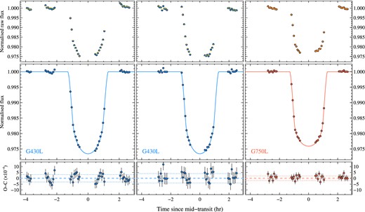
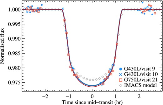
HST STIS normalized white-light curves based on visits 9, 10 and 21 (left to right). Blue and red symbols indicate G430L and G750L gratings, respectively. Top panels: normalized raw flux with the best-fitting model (yellow dots); Middle panels: detrended light curves along with the best-fitting transit model (Mandel & Agol 2002) plotted with continuous lines; lower panels: light-curve residuals and a 1σ level (dotted lines).
The effect of stellar activity on the transmission spectrum can be taken into account by computing corrections of the measured |${{{R_{\rm p}/R_\ast }}}$| provided the flux level of the star is known for each epoch of interest, as detailed in Sing et al. (2011) and Huitson et al. (2013). Unfortunately, our HST and Spitzer observations occurred at epochs when our ground-based photometry was thin. However, it enables an evaluation of the uncertainties associated with the effect of stellar activity. Both the photometry in the relevant season, and the amplitude of the variation in previous seasons, suggest that the star flux varies by not more than about 1 per cent peak to peak or an rms of 0.3 per cent as measured from the ground-based light curve. Therefore, we choose to translate this value into an added uncertainty on the relative planet-to-star radius ratio (with a typical value of |${\Delta} {{{R_{\rm p}/R_\ast}}} \simeq 0.000 \, 22$|) when presenting the transmission spectrum from all instruments following equation 5 of Sing et al. (2011).
3 ANALYSIS
We adopt similar analysis methods for the whole HST survey that are similar to the approach detailed in Sing et al. (2011, 2013), Huitson et al. (2013) and Nikolov et al. (2014), which we also describe briefly here. We fit each HST and Spitzer transit light curve in flux employing a two-component model that consists of a transit model multiplied by a systematics model. The transit model is based on the complete analytic formula given in Mandel & Agol (2002), which in addition to the central transit times (TC) and orbital period (P), is a function of the orbital inclination (i), normalized planet semimajor axis (a/R*) and planet-to-star radius ratio (Rp/R*). The systematics models are different for the HST and Spitzer data and are detailed below. We initially fixed the orbital period of the planet to its literature value (Gillon et al. 2009) before being updated to the final value reported in Section 3.2.
3.0.1 STIS white light-curve modelling
The three STIS white-light curves were fitted simultaneously with common inclination, semimajor axis and a planet-to-star radius contrast. We internally linked the radius parameter in our code to produce joint value for both G430L gratings. For the white-light curves, we fit these parameters simultaneously assuming flat priors. We use the resulting parameters from both G430L and G750L white-light curves in conjunction with literature results to refine WASP-6's system parameters and transit ephemeris (see Fig. 4).
We take into account the stellar limb darkening of the parent star in our code adopting the four parameter non-linear limb-darkening law. We calculate the relevant coefficients with ATLAS stellar models following Sing (2010) and adopting the stellar parameters Teff = 5375 K, log g = 4.61 and [Fe/H] = −0.2 from Gillon et al. (2009) and Doyle et al. (2013). We choose to rely on theoretically derived stellar limb-darkening coefficients from 1D stellar models, rather than to fit for them in the data in order to reduce the number of free parameters in the fit (see Table 1). Furthermore, this approach also eliminates the well-known wavelength-dependent degeneracy of limb darkening with transit depth (Sing et al. 2008).
Orbit-to-orbit flux corrections were applied to the STIS data similar to past HST studies by fitting a fourth-order polynomial of the spacecraft orbital phase (ϕt). In addition, we find that the systematics vary from orbit-to-orbit (i.e. dependence with time, t), which is a known effect from previous STIS studies as well as with the detector positions of the spectra, as determined by the spectral trace orientation (x, y) obtained from the APPAL task in iraf and the wavelength shift (ω) of each spectrum of the time series, compared to a reference. Model selection was investigated as in Nikolov et al. (2014) including (i) polynomials of degrees higher than fourth order for the HST orbital phase, and (ii) additional terms to the planet orbital phase, spectral shifts and traces. Such models were found statistically unjustified based on the Bayesian information criterion (BIC; Schwarz 1978). For instance, we found that fifth- or sixth-order polynomials of HST orbital phase gave BICs of 149 and 153, respectively. These values are much higher compared to the value produced by the most favourable model which includes a fourth-order polynomial, a linear time term and x (BIC of 96). The final systematics model for the red data include a fourth-order polynomial of HST orbital phase, a linear time term, and ω with BIC of 77. For comparison, a systematics model of a fourth-order polynomial of HST orbital phase, a linear time term, ω and ω2 gave BIC of 83. Finally, we find that the fitted transit parameters are very well constrained (including the transit depth) and are consistent regardless of the exact systematics model (see Fig. 5).
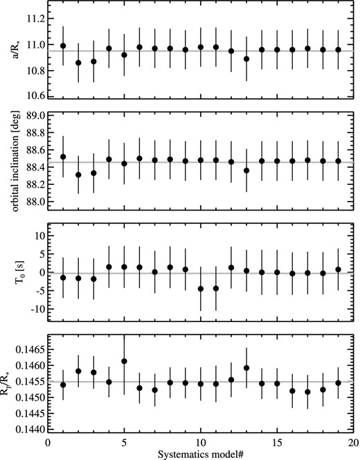
Transit parameters as a function of systematics model for STIS G750L data with uncertainties derived assuming photon noise only (i.e. not rescaled). The horizontal axis indicates the systematics model identification number as follows: (1) |$\phi _{t} + \phi ^{2}_{t}+ \phi ^{3}_{t}+ \phi ^{4}_{t}$|; (2) |$\phi _{t} + \phi ^{2}_{t}+ \phi ^{3}_{t}+ \phi ^{4}_{t}+ \phi ^{5}_{t}$|; (3) |$\phi _{t} + \phi ^{2}_{t}+ \phi ^{3}_{t}+ \phi ^{4}_{t}+ \phi ^{5}_{t}+ \phi ^{6}_{t}$|; (4) |$\phi _{t} + \phi ^{2}_{t}+ \phi ^{3}_{t}+ \phi ^{4}_{t} + t$|; (5) |$\phi _{t} + \phi ^{2}_{t}+ \phi ^{3}_{t}+ \phi ^{4}_{t} + t + t^2$|; (6) |$\phi _{t} + \phi ^{2}_{t}+ \phi ^{3}_{t}+ \phi ^{4}_{t} + t^2$|; (7) |$\phi _{t} + \phi ^{2}_{t}+ \phi ^{3}_{t}+ \phi ^{4}_{t} + t + x$|; (8) |$\phi _{t} + \phi ^{2}_{t}+ \phi ^{3}_{t}+ \phi ^{4}_{t} + t + y$|; (9) |$\phi _{t} + \phi ^{2}_{t}+ \phi ^{3}_{t}+ \phi ^{4}_{t} + t + \omega$|; (10) |$\phi _{t} + \phi ^{2}_{t}+ \phi ^{3}_{t}+ \phi ^{4}_{t} + t + x+x^2$|; (11) |$\phi _{t} + \phi ^{2}_{t}+ \phi ^{3}_{t}+ \phi ^{4}_{t} + t + x + x^2 + x^3$|; (12) |$\phi _{t} + \phi ^{2}_{t}+ \phi ^{3}_{t}+ \phi ^{4}_{t} + t + y + y^2$|; (13) |$\phi _{t} + \phi ^{2}_{t}+ \phi ^{3}_{t}+ \phi ^{4}_{t} + t + x + y^2 + y^3$|; (14) |$\phi _{t} + \phi ^{2}_{t}+ \phi ^{3}_{t}+ \phi ^{4}_{t} + t + \omega + \omega ^2$|; (15) |$\phi _{t} + \phi ^{2}_{t}+ \phi ^{3}_{t}+ \phi ^{4}_{t} + t + x + x^2 + x^3$|; (16) |$\phi _{t} + \phi ^{2}_{t}+ \phi ^{3}_{t}+ \phi ^{4}_{t} + t + x + y + \omega$|; (17) |$\phi _{t} + \phi ^{2}_{t}+ \phi ^{3}_{t}+ \phi ^{4}_{t} + t + x + x^2 + x^3$|; (18) |$\phi _{t} + \phi ^{2}_{t}+ \phi ^{3}_{t}+ \phi ^{4}_{t} + t + x +\omega$|; (19) |$\phi _{t} + \phi ^{2}_{t}+ \phi ^{3}_{t}+ \phi ^{4}_{t} + t + y + \omega$|
The errors on each photometric data point from the HST time series were initially set to the pipeline values, which are dominated by photon noise with readout noise also taken into account. We determine the best-fitting parameters simultaneously with the Levenberg–Marquardt least-squares algorithm as implemented in the idl3mpfit4 package (Markwardt 2009) using the unbinned data. The final results for the uncertainties of the fitted parameters were taken from mpfit after we rescaled the errors per data point based on the standard deviation of the residuals. We compare the residual dispersion of each white light curve to the expected one from photon noise. The data is found to reach ∼77, ∼65 and ∼89 per cent of the photon noise limit for visits 9, 10 and 21, respectively, which is similar earlier STIS studies (Huitson et al. 2013; Sing et al. 2013; Nikolov et al. 2014).
Finally, we also explored the dependence of the fitted transit parameters of the adopted systematics model. In these fits, we report the fitted parameters with uncertainties assuming pure photon noise and no rescaling. A summary of our results for grating G750L is shown in Fig. 5. We find that the fitted parameters in each STIS grating remain practically the same regardless the systematics model. These results are similar to what was found in Nikolov et al. (2014).
3.0.2 Spitzer IRAC light-curve fits
We model the 3.6 and 4.5 μm transit light curves following standard procedures for warm Spitzer. In particular, we correct the intrapixel sensitivity-induced flux variations by fitting a polynomial function of the stellar centroid position (Charbonneau et al. 2005, 2008; Reach et al. 2005; Knutson et al. 2008). As discussed in Lewis et al. (2013), this method has been proved to work reasonably well on short time-scales (<10 h) where the variations in the stellar centroid position are small (<0.2 pixels). These two conditions are satisfied for the WASP-6 data analysed in our study. To correct for systematic effects, we used a parametric model of the form: f(t) = a0 + a1x + a2x2 + a3y + a4y2 + a5xy + a6t, where f(t) is the stellar flux as function of time, x and y are the positions of the stellar centroid on the detector, t is time and a0 to a6 are the free parameters of the fit. The limb darkening of the star was taken into account by a non-linear law, assuming an ATLAS stellar atmosphere and the recipe of Sing (2010). Both light curves were jointly fitted with all parameters set free except to the orbital inclination and semimajor axis (as a/R*). These two parameters were linked to result to single values. The best-fitting orbital parameters were found to be in excellent agreement (within 1σ) with the results from the STIS white-light-curve analysis. We estimated the degree of red noise using the Carter & Winn (2009) wavelet method finding white and red noise components σw = 0.0068 and σr = 0.000 12 for the 3.6 μm data and σw = 0.0094 and σr = 0.000 16 for the 4.5 μm light curve, respectively. The values for Rp/R* used for the transmission spectrum were measured by fixing the system parameters, namely the orbital period, a/R*, i and the central transit times to their best-fitting values and the limb-darkening coefficients were kept fixed to their theoretical values.
We also performed two tests to explore the impact of incomplete Spitzer IRAC transit light curves on the measured system parameters. We obtained the 3.6 and 4.5 μm full-transit coverage light curves of WASP-31 reported in Sing et al. (2015). The data has similar noise properties and has been reduced with the same pipeline as our WASP-6 data. The WASP-31 light curves conveniently include enough out-of-transit baseline on both ends of the transits to evaluate measuring full versus half transits. We trimmed 20 × n-minute sections (n = 1, 7) from the beginning of the observation to produce half-transit light curves until we pass the transit central time. We fitted each light curve following the same methodology adopted for the WASP-6 IRAC data. In the first test, we fitted for all transit and systematics parameters while in the second we fixed a/R*, the orbital inclination and the central times to their best-fitting values measured using the whole data sets. We find that the first test gave transit parameters consistent with each other within 1σ when using light curves containing the transit central time. The largest variation is found for the values of transit mid-time and a/R*. The radius values (i.e. Rp/R*) for both channels remained within 1σ with increasing errors due to the smaller light-curve sections used. We measure rms of Rp/R* for both channels to be 0.0025 and 0.0016, respectively. The second test aimed to explore the reliability of the measured Rp/R* from half transits. We find this parameter more stable than in the first test withrms of Rp/R* values of 0.0013 and 0.0010 for the 3.6 and 4.5 μm light curves, respectively. We conclude that the Rp/R* values measured with our fitting code from incomplete Spitzer IRAC 3.6 and 4.5 μm can be trusted as long as the data include the transit mid-time and the fitting is done by fixing the system parameters and limb-darkening coefficients to well-determined values. As the WASP-6 light curves are only missing pre-ingress data, the obtained planet radii should be reliable.
3.1 System parameters and transit ephemeris
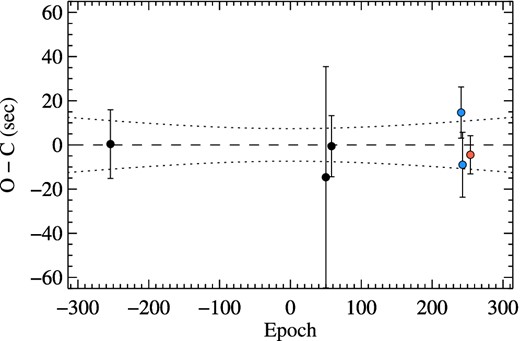
Observed minus computed (O−C) transit times for WASP-6b, based on our HST STIS measurements (blue and red dots) and observations reported in the literature (black dots) and the best-fitting orbital period and central transit time derived from our analysis. The dotted lines represent the computed 1σ uncertainty of the ephemeris.
1D limb-darkening coefficients employed in the fit to the STIS white light curves and results for the Rp/R*, transit times and residual scatter in parts per million (ppm).
| Visit ID | Instrument | c1 | c2 | c3 | c4 | Rp/R* | rms (ppm) |
|---|---|---|---|---|---|---|---|
| 9 | STIS/G430L | 0.6246 | −0.4673 | 1.2881 | −0.6067 | 0.147 26 ± 0.000 86 | 318 |
| 10 | STIS/G430L | 0.6246 | −0.4673 | 1.2881 | −0.6067 | 0.147 26 ± 0.000 86 | 372 |
| 21 | STIS/G750L | 0.6991 | −0.5421 | 1.0896 | −0.5187 | 0.145 20 ± 0.000 61 | 191 |
Transit mid-times and O−C residuals computed using our HST STIS light curves and results from the literature.
| Epoch | Central time | O−C | Reference |
|---|---|---|---|
| (BJDTDB) | (d) | ||
| −254 | 2454425.021657 ± 0.000180 | 0.000 004 | 1 |
| 50 | 2455446.766210 ± 0.000580 | −0.000 169 | 2 |
| 58 | 2455473.654392 ± 0.000160 | −0.000 007 | 3 |
| 241 | 2456088.718006 ± 0.000134 | 0.000 170 | 4 |
| 243 | 2456095.439737 ± 0.000170 | −0.000 104 | 4 |
| 254 | 2456132.410816 ± 0.000100 | −0.000 052 | 4 |
In addition, we refined the system parameters including the orbital inclination, i and normalized semimajor axis, (a/R*). We performed a joint fit to the three HST white-light curves finding i = 88.57 ± 0| $_{.}^{\circ}$|29 and a/R* =11.05 ± 0.17.
3.2 An evaluation of the stellar activity from the HST data
The overlapping region between the two STIS gratings offers the opportunity to measure the photometric variability of the host star over the time interval of 40 d covered by the three HST visits, as significant stellar activity from stellar spots would change the measured transit radii. We used three light curves from the range 5400–5650 Å (i.e. avoiding the rapid sensitivity change in G750L from 5250–5400 Å, see fig. 1 from Nikolov et al. 2014) and measured the quantity |${{{R_{\rm p}/R_\ast }}}$| from a fit, keeping the system parameters, ephemeris and limb darkening to their best-fitting white light values and theoretical coefficients, respectively. The result is shown in Fig. 7. The standard deviation in |${{{R_{\rm p}/R_\ast }}}$| is ∼2 × 10⁻⁴ and the translated flux variation of the star is <0.3 per cent, which is in agreement with our ground-based result discussed in Section 2.3 and the result of Jordán et al. (2013) who found a peak-to-peak amplitude <4 mmag. Our result suggests that the three HST visits occurred at similar stellar flux levels implying no significant offset between the blue and red STIS sections of the transmission spectrum. Finally, the very similar radius values for the two blue visits obtained six days apart imply the lack of variability related with the planetary atmosphere itself.
3.3 Fits to transmission spectra
The primary science goal of this study is to construct a low-resolution optical to near-infrared transmission spectrum of WASP-6 b and to pursue the prediction of strong optical absorbers such as sodium (observed in the Na i doublet at λ = 5893 Å), potassium (K i doublet at λ = 7684 Å) and water vapour (e.g. in 1.45 μm band) or alternatively high-altitude atmospheric haze (in optical scattering), and/or a constant flat scattering at λ ≳ 1 μm. Light curves from various spectral bins were extracted from the STIS/G430L and G750L data to construct a broad-band transmission spectrum and to search for expected strong absorbers (see Figs 8 and 9).
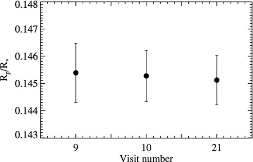
The three measured transit radii in a bin between 5250–5400 Å taken between the two STIS G430L visits and the STIS G750L visit. No significant difference in the transit depth is seen.
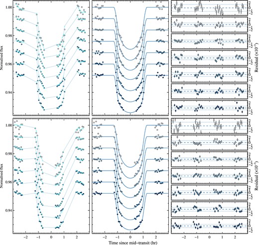
HST STIS G430L spectral bin light curves of visits 9 and 10. Left-hand panels: raw light curves and the best-fitting transit model, multiplied in flux by a systematics model shifted with an arbitrary constant. The points have been connected with lines for clarity and the light curves are presented in wavelength with the shortest wavelength bin displayed at the top and longest wavelength bin at the bottom. Middle panels: corrected light curves and the best-fitting transit model. Right-hand panels: observed minus computed residuals with 1σ error bars along with the standard deviation (dotted lines).
As pointed out in Pont et al. (2013), three issues must be addressed in order to place radius measurements on a common scale and build a transmission spectrum spanning a wide wavelength coverage: common orbital parameters, stellar limb darkening and the effect of stellar variability and star-spots. We take into account all of these issues in the analysis of the transmission spectrum from the HST and Spitzer data. In the light-curve fits, we fixed the system parameters, i.e. the orbital period (P), inclination (i), normalized semimajor axis (a/R*) and the transit mid-times (TC) to their values derived from the white-light-curve analysis (Section 3.2). We fit for the relative radius of the planet and the parameters describing the instrumental systematics. The activity of the parent star was taken into account by inflating the error bars of the measured Rp/R*of each spectral bin assuming stellar variability of 0.3 per cent. This number also takes into account the contribution of unocculted spots. The four non-linear limb-darkening coefficients were fixed to their theoretical values, computed from stellar models and taking into account the instrument response.
Similar to Sing et al. (2013) and Nikolov et al. (2014), we performed the modelling of systematic errors in each spectral bin by two methods. In the first method, we fit each light curve independently with a parametrized model. In the second approach, we removed the common-mode systematics from each spectral bin before fitting for residual trends with a parametrized model but with fewer parameters. The common-mode trends were extracted at the white-light-curve analysis by dividing the white-light raw flux in each grating to the best-fitting transit model constrained from a joint fit to the three STIS data sets. It was found that this method reduces the amplitude of the breathing systematics. We found that for the WASP-6 data the common-mode approach generally worked better for the G430L data than for the G750L spectral light curves. This is expected as the G430L spectral light curves exhibit very similar systematic trends which is not the case for the G750L spectral light curves. A visual inspection of the out-of-transit data on Figs 8 and 9 reveals this fact. As found in Sing et al. (2013) for the WASP-12b and Nikolov et al. (2014) for the HAT-P-1b STIS transit data, we find that the transmission spectra from both methods show little difference (i.e. deviations in the Rp/R*within 1σ of their fitted values). For consistency, we choose to report the final transmission spectrum from the first method. The broad-band spectrum results are provided in Table 3 and displayed in Fig. 10.
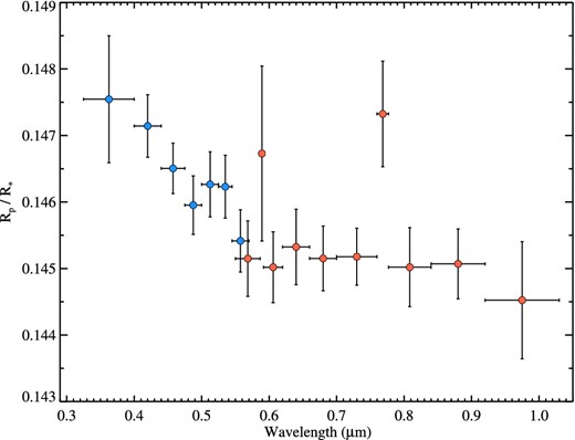
Combined HST STIS G430L and G750L transmission spectrum of WASP-6b (blue and red dots, respectively).
Measured Rp/R* from fits to the G430L and G750L transit light curves and limb-darkening coefficients.
| Wavelength (Å) | Rp/R* | c1 | c2 | c3 | c4 |
|---|---|---|---|---|---|
| Visit 9 and 10 | |||||
| 3250–4000 | 0.147 55 ± 0.000 98 | 0.5049 | −0.6907 | 1.9020 | −0.7850 |
| 4000–4400 | 0.147 14 ± 0.000 52 | 0.5077 | −0.6398 | 1.8008 | −0.7416 |
| 4400–4750 | 0.146 50 ± 0.000 44 | 0.6469 | −0.8914 | 1.9172 | −0.7695 |
| 4750–5000 | 0.145 95 ± 0.000 49 | 0.5652 | −0.3541 | 1.2492 | −0.5989 |
| 5000–5250 | 0.146 27 ± 0.000 54 | 0.5392 | −0.2004 | 1.0534 | −0.5399 |
| 5250–5450 | 0.146 23 ± 0.000 52 | 0.6247 | −0.4675 | 1.2882 | −0.6067 |
| 5450–5700 | 0.145 41 ± 0.000 52 | 0.5404 | −0.2277 | 1.0662 | −0.5468 |
| Visit 21 | |||||
| 5500–5868 | 0.145 15 ± 0.000 61 | 0.6081 | −0.4022 | 1.2199 | −0.5927 |
| 5868–5918 | 0.1467 ± 0.0013 | 0.5750 | −0.2207 | 0.9647 | −0.5064 |
| 5918–6200 | 0.145 02 ± 0.000 58 | 0.6241 | −0.3386 | 1.0136 | −0.5079 |
| 6200–6600 | 0.145 32 ± 0.000 61 | 0.6552 | −0.4611 | 1.1582 | −0.5801 |
| 6600–7000 | 0.145 15 ± 0.000 53 | 0.6791 | −0.4802 | 1.0974 | −0.5326 |
| 7000–7599 | 0.145 18 ± 0.000 48 | 0.7361 | −0.6490 | 1.2003 | −0.5554 |
| 7599–7769 | 0.147 32 ± 0.000 82 | 0.7099 | −0.5449 | 1.0219 | −0.4847 |
| 7769–8400 | 0.145 02 ± 0.000 63 | 0.7578 | −0.7132 | 1.2070 | −0.5521 |
| 8400–9200 | 0.145 07 ± 0.000 57 | 0.7005 | −0.5541 | 0.9344 | −0.4345 |
| 9200–10 300 | 0.144 52 ± 0.000 91 | 0.7221 | −0.6191 | 0.9967 | −0.4582 |
| 36 000 | 0.1404 ± 0.0014 | 0.4434 | −0.2253 | 0.1829 | −0.0717 |
| 45 000 | 0.1405 ± 0.0015 | 0.5356 | −0.6254 | 0.6113 | −0.2243 |
4 DISCUSSION
4.1 A search for narrow-band spectral signatures
We performed a thorough search for narrow-band absorption features including the expected signatures of Na, K, Hα and Hβ. In the context of the HST survey, sodium has been detected by Nikolov et al. (2014) in the HAT-P-1b exoplanet using a 30 Å bin and potassium has been detected in the WASP-31b atmosphere by Sing et al. (2015) using 75 Å bin. In the case of WASP-6b, we followed the methods described in Nikolov et al. (2014) and used a set of six bands centred on the expected features with widths from 15 to 90 Å with step of 15 Å for Na, Hα and Hβ and twice larger for the potassium feature. We find only tentative evidence for sodium and potassium line cores with the largest significance levels of 1.2σ and 2.7σ in 50 and 170 Å bins, respectively. We also searched but did not find evidence for Na and K pressure-broadened line wings. Finally, we find also no evidence for Hα nor Hβ.
4.2 Comparison to existing cloud-free theoretical models
We compare our transmission spectrum to a variety of different cloud-free atmospheric models based on the formalism of Burrows et al. (2010), Howe & Burrows (2012) and Fortney et al. (2008, 2010). We averaged the model within the transmission spectrum wavelength bins and fitted these theoretical values to the data with a single free parameter that controls their vertical position. We compute the χ2 statistic to quantify model selection with the number of degrees of freedom for each model given by ν = N − m, where N is the number of data points (21) and m is the number of fitted parameters.
The models from Burrows et al. (2010) and Howe & Burrows (2012) assume 1D dayside temperature–pressure (T–P) profile with stellar irradiation, in radiative, chemical, and hydrostatic equilibrium. Chemical mixing ratios and corresponding opacities assume solar metallicity and local thermodynamical chemical equilibrium accounting for condensation with no ionization, using the opacity data base from Sharp & Burrows (2007) and the equilibrium chemical abundances from Burrows & Sharp (1999) and Burrows et al. (2001).
The models based on Fortney et al. (2008, 2010) include a self-consistent treatment of radiative transfer and chemical equilibrium of neutral and ionic species. Chemical mixing ratios and opacities assume solar metallicity and local chemical equilibrium, accounting for condensation and thermal ionization though no photochemistry (Lodders 1999, 2002, 2009; Lodders & Fegley 2002, 2006; Visscher, Lodders & Fegley 2006; Freedman, Marley & Lodders 2008). In addition to isothermal models, transmission spectra were calculated using 1D temperature–pressure (T–P) profiles for the dayside, as well as an overall cooler planetary-averaged profile. Models were also generated both with and without the inclusion of TiO and VO opacities. Because each of the aforementioned models started at wavelength λ = 3500 Å (due to a restriction of the employed opacity data base), we extrapolated the models in the range 2700–3500 Å to enable self-content comparisons to the bluest STIS measurements along with all models.
As it becomes apparent from Table 4, all of the cloud-free models struggle to represent the observed transmission spectrum of WASP-6b, providing poor fits (see Fig. 11).
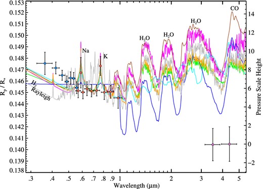
WASP-6b transmission spectrum compared to seven different cloud-free atmosphere models listed in Table 4, including Burrows-Dayside1200K-3 ×solar (brown), Burrows-Isoth.1200K-high-CO (cyan), Burrows-Isoth.1200K-ExtraAbsorber (blue), Fortney-Isoth.1000K (green), Fortney-Isoth.1500K-noTiO/VO (magenta), Fortney-PlanetAveraged1200K (orange) and Fortney-Isoth.1500K-withTiO/VO (grey). All these models hardly reproduce the two Spitzer measurements. Prominent absorption features are labelled.
Model (cloud-free) selection fit statistics (N = 19).
| Models | χ2 | ν | BIC |
|---|---|---|---|
| Burrows-Isoth.1200K-ExtraAbsorber | 55.9 | 17 | 58.9 |
| Fortney-Isoth.1000K | 74.1 | 18 | 77.0 |
| Fortney-PlanetAveraged1200K | 81.9 | 18 | 84.8 |
| Burrows-Isoth.1200K-high-CO | 82.7 | 17 | 85.6 |
| Burrows-Dayside1200K-3 ×solar | 102.9 | 18 | 105.9 |
| Fortney-Isoth.1500K-noTiO/VO | 107.6 | 18 | 110.5 |
| Fortney-Isoth.1500K-withTiO/VO | 124.4 | 18 | 127.4 |
4.3 Interpreting the transmission spectrum with aerosols
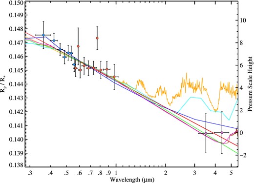
An overall slope in the transmission spectrum is a main atmospheric characteristic, spanning 0.0071(Rp/R*), corresponding to ∼9 atmospheric pressure scaleheights (|$H = \frac{kT}{\mu g} = 492\pm 24$| km, assuming |$T = 1194^{+58}_{-57}$| K and g = 8.710 ± 0.012) from the optical to the near-infrared (see Fig. 11).
4.3.1 Rayleigh scattering
4.3.2 Mie scattering dust
Good fits to the data are possible assuming a significant opacity from aerosols, i.e. colloids of fine solid particles or liquid droplets in a gas. Aerosol-bearing models assuming Mie theory can fit the observed slope in the spectrum of WASP-6b. Such materials can be produced from condensate dust species or alternatively from photochemistry (Marley et al. 2013). Given the ∼1000 K planetary temperatures of WASP-6b, the prime condensate candidate materials include MgSiO3 (enstatite), Mg2SiO4 (forsterite), sulphides and chlorides of the alkali metals Na and K (Lodders 2003; Morley et al. 2012). Compared to the enstatite and forsterite, the alkali sulphides and chlorides are expected to be considerably less abundant in solar-composition atmospheres.
A variety of different atmospheric models were tested assuming aerosols are the main spectral feature throughout the transmission spectrum. The optical properties (i.e. complex indices of refraction as a function of wavelength) were compiled in order of decreasing condensation temperature from 1316 to 90 K for MgSiO3, Fe-poor Mg2SiO4, Na2S, MnS, KCl and Titan tholin with all condensates at pressures 10−3 bar (Huffman & Wild 1967; Egan & Hilgeman 1975; Khare et al. 1984; Palik 1998; Ramirez et al. 2002; Khachai et al. 2009; Zeidler et al. 2011). As in Sing et al. (2013), cross-sections as a function of wavelength were computed with Mie theory which were then used to compute the transmission spectra using the expression for the planetary altitude derived in Lecavelier Des Etangs et al. (2008a). In all fits, we excluded the radius measurements corresponding to the sodium and potassium spectral bins, as these are not predicted by the Mie scattering theoretical models.
First, we assumed a grain size a and planetary temperature equal to the equilibrium temperature and fit for the baseline radius. This approximation is valid given the fact that the cross-section distribution is dominated by the largest grain sizes with σ ∝ a6 (Lecavelier Des Etangs et al. 2008a).
Similar to what was found in Sing et al. (2013), when fitting the data for the grain size, temperature and baseline radius simultaneously, a degeneracy between the first two parameters becomes evident. This is not unusual as the slope of the transmission spectrum constrains the quantity αT, with the grain size included in the term α. In the case of WASP-6b, we found that Mie scattering model fitted with Fe-poor Mg2SiO4 favoured sub-micron grain sizes and higher temperatures (∼1400 K). Similar quality fits with models containing MgSiO3, KCl and Na2S were also found at a temperature of 1145 K and grain size around 0.1 μm (Fig. 12 and Table 5). The similarity between a pure Rayleigh scattering and Mie scattering models with sub-micron grain sizes from the optical to the near-IR regime is not unusual, as the Mie theory reduces to Rayleigh scattering for particles with sizes much smaller than the wavelength of the light and for compositions with low imaginary components of the index of refraction in the wavelength range considered, as is the case with KCl and MgSiO3.
Broad-band transmission spectrum of WASP-6b compared (without the sodium and potassium measurements) to seven different aerosol models including: Rayleigh scattering (red), Mie scattering KCl (green), MgSiO3 (magenta), Fe-poor Mg2SiO4 (brown), a model with enhanced Rayleigh scattering component with a cross-section 103 times that of H2 Fortney.noTiO-EnhancedRayleigh (orange), Na2S (blue) and Titan tholin (cyan).
Model (Mie scattering) selection fit statistics for the complete transmission spectrum (N = 17).
| Models | χ2 | ν | BIC |
|---|---|---|---|
| Rayleigh | 6.1 | 15 | 11.7 |
| Mie scattering MgSiO3 or KCl | 6.7 | 15 | 12.4 |
| Mie scattering Mg2SiO4 (Fe-poor) | 6.8 | 15 | 12.5 |
| Mie scattering Na2S | 6.9 | 15 | 12.5 |
| Titan tholin | 9.9 | 15 | 15.5 |
| Mie scattering MnS | 11.4 | 15 | 17.1 |
| Fortney.noTiO-EnhancedRayleigh | 14.0 | 16 | 16.9 |
| Fortney.noTiO-CloudDeck | 88.2 | 16 | 91.0 |
We also explored the possibility to constrain the condensate and its grain size at lower temperature of 973 K, which we found assuming Rayleigh scattering when fitting the slope of the transmission spectrum. Fitting for the baseline radius and grain size a, we found that Fe-poor Mg2SiO4, MgSiO3 and KCl are the most favoured materials with grain size a = 0.1 μm (χ2 = 6.3 for ν = 15).
We also estimated condensate grain sizes assuming a planetary temperature of 1145 K and fitting for a and the baseline radius. This temperature is similar to the condensation temperature of most of the condensates listed in Table 5. We find that MgSiO3, KCl, Fe-poor Mg2SiO4 and Na2S are the first four most favoured materials with grain sizes of ∼ 0.1 μm.
Finally, we examined how our results would change when the optical data is modelled, i.e. excluding the two IRAC measurements. We also excluded the sodium and potassium measurements and fixed the planet temperature to 1145 K and fitted for the grain size and the baseline radius. We find grain size a ∼ 0.1 μm for all condensates and the model containing MnS as the most favoured (Table 6).
Model fit statistics for the optical spectrum (N = 15).
| Models | χ2 | ν | BIC |
|---|---|---|---|
| Mie scattering MnS | 5.1 | 13 | 10.6 |
| Rayleigh | 5.9 | 13 | 11.3 |
| Fortney.noTiO-EnhancedRayleigh | 6.3 | 14 | 9.0 |
| Mie scattering MgSiO3, Na2S or KCl | 6.4 | 13 | 11.8 |
| Titan tholin | 6.5 | 13 | 11.9 |
| Mie scattering Mg2SiO4 (Fe-poor) | 6.6 | 13 | 12.0 |
| Fortney.noTiO-CloudDeck | 88.2 | 14 | 50.7 |
System parameters for WASP-6 and HD 189733.
| Property | WASP-6 | HD 189733 |
|---|---|---|
| Teff, K | 5375 ± 65 | 5050 ± 50 |
| log g, cm s−2 | 4.61 ± 0.07 | 4.61 ± 0.03 |
| [Fe/H], dex | −0.20 ± 0.09 | −0.03 ± 0.05 |
| |$P, {\rm {{\rm d}}}$| | 3.361 | 2.219 |
| |$a, {\rm {{\rm au}}}$| | 0.042 | 0.031 |
| e | 0 | 0 |
| g | 8.71 ± 0.01 | 21.5 ± 1.2 |
| Teq | 1145 ± 23 | 1191 ± 20 |
| H, km | 492 | 199 |
4.3.3 High-altitude haze and lower altitude clouds
We also compared the transmission spectrum of WASP-6b with a suite of Fortney et al. (2010) atmospheric models with either an artificially added Rayleigh scattering component simulating a scattering haze, or an added ‘cloud deck’ produced by a grey flat line at specific altitude. We performed comparison to these models as they can help better understand our observational results, as clouds and hazes can mask or completely block the expected atomic and molecular features in a transmission spectrum depending on the altitude distribution and particle size. We find that a fit to the data of a 1200 K model without TiO/VO and with a Rayleigh scattering component with a cross-section 1000 times that of H2 gave χ2 of 14.0 for ν = 16. In this model, the optical spectrum is dominated by Rayleigh scattering with H2O features evident in the near-IR (see Fig. 12).
In the Solar system planets, the scaleheight of haze is often smaller than the scaleheight of the atmosphere itself, because of sedimentation and the structure of the vertical mixing. That would result in a smaller Rayleigh slope for the haze signature in the transmission spectrum. It would also add a gas-to-grain scaleheight ratio factor in equation 1 of Lecavelier Des Etangs et al. (2008a), thus severing the relation between the measured slope and the temperature. A typical gas-to-grain scaleheight ratio in the Solar system is 3, which implies a non-negligible correction.
4.4 The atmosphere of WASP-6b
The best-fitting atmospheric models to our data are those containing opacity from Mie or Rayleigh scattering as summarized in Tables 4 and 5. All of the cloud-free models have been found to produce unsatisfactory fits indicating low level of molecular absorption in our data. Rayleigh scattering can potentially be produced by molecular hydrogen, a potential scenario explored for HD 209458b (Lecavelier Des Etangs et al. 2008b). However, molecular hydrogen is disfavoured for WASP-6b by the lack of pressure-broadened line wings in its transmission spectrum and the low altitudes of any molecular features as apparent in Fig. 11. Rayleigh scattering implies temperatures of 978 ± 217 or 973 ± 144 K based on a fit to the optical or complete spectrum, respectively. These results are consistent with the estimated planet equilibrium temperature of Teq = 1145 ± 23 K at ∼1σ confidence level.
The first five best-fitting Mie scattering aerosol models are practically indistinguishable in quality between each other providing good representation of the observed transmission spectrum (Table 5). A confident constraint on the composition of the scattering material is hampered by the grain size–temperature degeneracy and the lack of wide spectral coverage. Near-future UV data could potentially resolve these issues, as the Mie scattering models become more distinct in that wavelength region (see Fig. 12). Despite the degeneracy, we find that the particle sizes of all models are sub-micron, regardless the temperature. On the other hand, near-infrared data such as WFC3 transit spectroscopy or broad-band JHK band transit photometry can bring more evidence for the hazy type of WASP-6b's atmosphere based on the strength of the water features expected at these regions.
4.4.1 Comparison to a ground-based result
Recently, Jordán et al. (2013) reported WASP-6b transmission spectrum with the Magellan IMACS instrument. With both space- and ground-based results in hand, we are in a position to perform a first rough comparison. We leave a detailed and self-consistent analysis for a future study and simply employ the HST STIS data to construct a transmission spectrum using the same spectral bins as in the ground-based study. When fitting the light curves, we fixed the system parameters to their best-fitting values. Furthermore, the quality of our data requires us to adopt the four-parameter limb-darkening law rather than the adopted quadratic law for the Magellan data set. We estimate the uncertainty of each data point in the time series assuming photon noise.
Compared to the HST transmission spectrum, the Magellan spectrum is found to be systematically offset with |${\Delta} {{{R_{\rm p}/R_\ast}}}\sim 0.007$| lower values. We find no evidence for the observed discrepancy to be due to the different system parameters (i.e. a/R* and i) nor the limb-darkening laws adopted. However, based on fig. 6 in Jordán et al. (2013) where white light curves are compared after subtracting the best-fitting systematics models, it can be seen that the final Magellan transit depth varies greatly between the different systematics models used. In particular, one can roughly estimate an average difference in the transit depth of ∼0.0017 between the white noise and ARMA models, which corresponds to a change of |${\Delta} {{{R_{\rm p}/R_\ast }}}= 0.0056$|. Thus, the differences between the systematics models employed in Jordán et al. (2013) could explain more than ∼80 per cent of the observed offset between the Magellan and HST transmission spectra. We therefore find that the potential source of discrepancy between the ground-based study and our results could be primarily linked with the subtracted systematics models of Jordán et al. (2013). Finally, the spectral bin between 5468–5647 Å is an overlapping region for the three HST and the Magellan data sets which offers the opportunity for a direct comparison of all data. Fig. 13 shows that the three STIS transit light curves obtained at three individual epochs are all in excellent agreement with each other, illustrating the measured HST transit depth is highly repeatable.
HST STIS light curves from bin 5468–5647 Å.
Therefore, the comparisons between both results are limited to only the shape of each spectrum, and not the absolute value of the parameter Rp/R*. When the HST and Magellan spectra are normalized to the same average level (Fig. 14), it becomes apparent that there is very good agreement in 15 out of 20 bandpasses, which agree at a 1σ level or less. Only in three of 20 channels, one finds a disagreement larger than 2σ (3.1, 2.7, and 3.2σ in channels 7215–7415, 7562–7734 and 7734–7988 Å, respectively). These regions coincide with several telluric lines (e.g. O2 and H2O), the variation of which on a time interval overlapping with the transit event could potentially introduce variation of the measured depth. The Magellan observation did suffer from changing weather conditions during the second half of the transit event as detailed in Jordán et al. (2013).
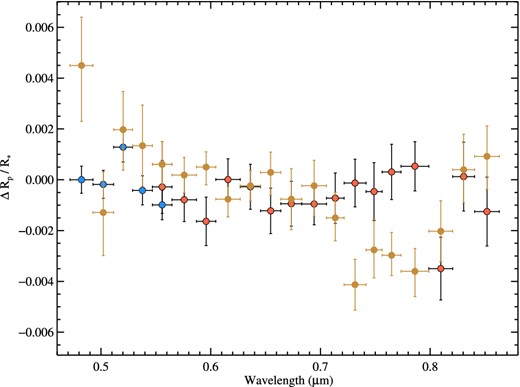
Comparison between the WASP-6b transmission spectrum from HST STIS and Magellan IMACS (blue, red and brown dots, respectively).
4.4.2 Comparison to HD 189733b
Complemented by the transmission spectra of HD 209458b and HD 189733b, the first results from the large HST programme coupled by Spitzer IRAC transit radii start building up an observational data base of hot-Jupiter atmospheres. The similarities and differences in the spectra and system parameters of the studied objects could potentially indicate distinct categories of gas giant atmospheres.
The optical transmission spectrum of WASP-6b shows some resemblance to that of HD 189733b (see Fig. 15). Both planets also have close zero-albedo equilibrium temperatures near 1200 K and are hosted by active stars with an overall less activity in WASP-6 as estimated from HARPS archival data (see Table 7). Both transmission spectra are characterized by larger optical to near-infrared radii indicating additional scattering in the optical region with featureless slopes and a lack of broad line wings of sodium and potassium which suggests high altitudes and low pressures (e.g. Désert et al. 2009, 2011; Pont et al. 2013 for HD 189733b). Instead, absorption from the narrow cores of the Na i and K i doublets are evidenced for HD 189733b in the medium resolution STIS data and the revised ACS data from Huitson et al. (2012) and Pont et al. (2013), respectively. In the case of WASP-6b, we find tentative evidence for narrow core of K i, but no evidence for Na i, which likely is due to the low resolution STIS G750L data.7 These facts are in accord with haze models, as hazes and clouds can reside at high altitudes which can mute or completely block the signatures of atomic and molecular features. Prime condensate candidates responsible for the hazes of HD 189733b and WASP-6b are considered to be silicate condensates such as enstatite (Lecavelier Des Etangs et al. 2008a; Pont et al. 2013).

Transmission spectrum of WASP-6b (blue) and HD 189733b (magenta), taken from Pont et al. (2013).
Significant differences between both planets and their host stars include a lower effective temperature (i.e. a later spectral type), higher metallicity and a factor of ∼3 larger surface gravity of HD189733 and its planet. In addition, HD 189733b's transmission spectrum exhibits a steeper scattering slope and relatively higher altitude for the hazes on WASP-6b (Fig. 15). Together with the planetary equilibrium temperature (Teq), the surface gravity (g) is an important parameter in determining the atmospheric scaleheight and hence the strength of absorption features in exoplanet transmission spectra. A higher surface gravity means that a given pressure corresponds to less mass. Since the clouds usually form at a given pressure level, but the effect of the haze is proportional to the mass, the haze signature in the transmission spectrum is expected to move higher compared to the clouds in a lower gravity atmosphere (that is part of the reason for instance that Saturn is very hazy while Jupiter is not). That effect goes in the right direction for WASP-6b versus HD189733b: the first will tend to have a stronger haze signature/deeper cloud deck in transmission. However, with a factor ∼3 in gravity, the difference would be ∼1 pressure scaleheight only, i.e. not enough to account for the full difference between WASP-6b and HD189733b.
Completing the transmission spectra in the near-IR range between 1 and 3 μm and improving the Spitzer measurement uncertainties will enable a more thorough comparison between the two planets’ atmospheres.
5 CONCLUSION
With a broad-coverage optical transmission spectrum measured from HST and Spitzer broad-band transit spectrophotometry, WASP-6b joins the small but highly valuable family of hot-Jupiter exoplanets with atmospheric constraints. We observe an overall spectrum characterized by a slope indicative of scattering by aerosols. The data point on the potassium spectral line is ∼2.7σ higher than the spectrum at that wavelength region. We find no evidence of pressure-broadened wings which is in agreement with the haze model as clouds and hazes can reside at high altitudes which can significantly mask or even completely block the signatures of collisionally broadened wings. Given the rather low temperature of WASP-6b, aerosol species are expected to originate from high-temperature condensates similar to these in the prototype HD 189733b. Given their condensation temperatures and the results from our analysis, MgSiO4, KCl, MgSiO3 and Na2S are candidate condensates.
WASP-6b is the second planet after HD 189733b which has equilibrium temperatures near ∼1200 K and shows prominent atmospheric scattering in the optical.
This work is based on observations with the NASA/ESA Hubble Space Telescope, obtained at the Space Telescope Science Institute (STScI) operated by AURA, Inc. This work is based in part on observations made with the Spitzer Space Telescope, which is operated by the Jet Propulsion Laboratory, California Institute of Technology under a contract with NASA. The research leading to these results has received funding from the European Research Council under the European Unions Seventh Framework Programme (FP7/2007-2013)/ERC grant agreement 336792. NN and DS acknowledge support from STFC consolidated grant ST/J0016/1. PW acknowledges support from STFC grant. All US-based co-authors acknowledge support from the Space Telescope Science Institute under HST-GO-12473 grants to their respective institutions.
CALSTIS comprises software tools developed for the calibration of STIS data (Katsanis & McGrath 1998) inside the iraf (Image Reduction and Analysis Facility; http://iraf.noao.edu/) environment.
As implemented in the idl|${{\tt box\_centroider.pro}}$|, provided on the Spitzer homepage: http://irsa.ipac.caltech.edu.
The acronym idl stands for Interactive Data Language.
Although a constant atmospheric temperature is not expected throughout the ∼9 pressure scaleheights, but is adopted here due to the lack of observations on the planet dayside spectrum.
Table 3 gives the wavelength bins and corresponding radius measurements for the most significant sodium and potassium detections. We note that future detailed direct comparison studies will have to choose a common band system, which potentially can be hampered by the specific resolution and S/N of each data set.
