


Abstract
Recent X-ray observations show absorbing winds with velocities up to mildly relativistic values of the order of ∼0.1c in a limited sample of six broad-line radio galaxies. They are observed as blueshifted Fe xxv–xxvi K-shell absorption lines, similarly to the ultrafast outflows (UFOs) reported in Seyferts and quasars. In this work we extend the search for such Fe K absorption lines to a larger sample of 26 radio-loud active galactic nuclei (AGN) observed with XMM–Newton and Suzaku. The sample is drawn from the Swift Burst Alert Telescope 58-month catalogue and blazars are excluded. X-ray bright Fanaroff–Riley Class II radio galaxies constitute the majority of the sources. Combining the results of this analysis with those in the literature we find that UFOs are detected in >27 per cent of the sources. However, correcting for the number of spectra with insufficient signal-to-noise ratio, we can estimate that the incidence of UFOs is this sample of radio-loud AGN is likely in the range f ≃ (50 ± 20) per cent. A photoionization modelling of the absorption lines with xstar allows us to estimate the distribution of their main parameters. The observed outflow velocities are broadly distributed between vout ≲ 1000 km s−1 and vout ≃ 0.4c, with mean and median values of vout ≃ 0.133c and vout ≃ 0.117c, respectively. The material is highly ionized, with an average ionization parameter of logξ ≃ 4.5 erg s−1 cm, and the column densities are larger than NH > 1022 cm−2. Overall, these characteristics are consistent with the presence of complex accretion disc winds in a significant fraction of radio-loud AGN and demonstrate that the presence of relativistic jets does not preclude the existence of winds, in accordance with several theoretical models.
1 INTRODUCTION
Increasing evidences show that most galaxies harbour a supermassive black hole (SMBH) at their centre (e.g. Ferrarese & Ford 2005). The accretion of material from these SMBHs provides the basic power source for active galactic nuclei (AGN). Depending on the ratio of their luminosity in radio and optical/X-rays, AGN are classified as radio-loud or radio-quiet (e.g. Terashima & Wilson 2003). Physically, this is related to the presence or absence of strong relativistic jets. The origin of this dichotomy is still debated and it is intimately linked to the mechanisms producing the jets, for instance the black hole spin (e.g. Sikora, Stawarz & Lasota 2007; Garofalo, Evans & Sambruna 2010; Tchekhovskoy & McKinney 2012).
In radio-loud AGN the highly collimated relativistic jets are frequently observed at radio, optical and X-rays. They can travel for very long distances, impacting areas far away from the centre of these galaxies. Until very recently, this was the main known mechanism for the deposition of mechanical energy from the SMBH into the host galaxy environment in radio-loud sources, contributing to the AGN cosmological feedback (e.g. Fabian 2012). Deep X-ray observations changed this view, showing an increasing evidence for accretion disc winds/outflows in this class of sources as well.
For instance, the systematic analysis of the Suzaku spectra of a small sample of five bright broad-line radio galaxies (BLRGs) performed by Tombesi et al. (2010a) showed significant blueshifted Fe xxv/xxvi K-shell absorption lines at E > 7 keV at least in three of them, namely 3C 111, 3C 120 and 3C 390.3. They imply an origin from highly ionized and high column density gas outflowing with mildly relativistic velocities of the order of 10 per cent of the speed of light. Successive studies confirmed these findings and found similar outflows also in 3C 445 and 4C+74.26 (Reeves et al. 2010; Ballo et al. 2011; Braito et al. 2011; Tombesi et al. 2011a, 2012b, 2013b; Gofford et al. 2013). The slower (vout ∼ 100–1000 km s−1) and less ionized warm absorbers have also been detected in the soft X-ray spectra of some bright BLRGs (Reynolds 1997; Ballantyne 2005; Reeves et al. 2009b, 2010; Torresi et al. 2010, 2012; Braito et al. 2011). These observations indicate that, at least for some radio-loud AGN, the presence of relativistic jets does not preclude the existence of winds and the two might possibly be linked (e.g. Tombesi et al. 2012b, 2013b; Fukumura et al. 2014).
The characteristics of these winds are similar to the ultrafast outflows (UFOs) with velocities vout ≥ 10 000 km s−1 observed in ∼40 per cent of radio-quiet AGN (e.g. Chartas et al. 2002, 2009; Chartas, Brandt & Gallagher 2003; Pounds et al. 2003; Dadina et al. 2005; Markowitz, Reeves & Braito 2006; Braito et al. 2007; Papadakis et al. 2007; Cappi et al. 2009; Reeves et al. 2009a; Tombesi et al. 2010b, 2011b; Giustini et al. 2011; Gofford et al. 2011, 2013; Lobban et al. 2011; Dauser et al. 2012; Lanzuisi et al. 2012; Patrick et al. 2012; Gupta et al. 2013). The mechanical power of these UFOs seems to be high enough to influence the host galaxy environment (Tombesi et al. 2012a, 2013a), in accordance with simulations of SMBH–galaxy feedback driven by AGN winds/outflows (e.g. King & Pounds 2003, 2014; Di Matteo, Springel & Hernquist 2005; Hopkins & Elvis 2010; King 2010; Ostriker et al. 2010; Gaspari et al. 2011a,b; Gaspari, Ruszkowski & Sharma 2012; Zubovas & King 2012, 2013; Wagner, Umemura & Bicknell 2013).
The typical location of the UFOs is estimated to be in the range ∼102–104rs (rs = GMBH/c2) from the central SMBH, indicating a direct association with winds originating from the accretion disc (e.g. Tombesi et al. 2012a, 2013a). Their high ionization levels and velocities are, to date, consistent with both radiation pressure and magnetohydrodynamic (MHD) processes contributing to the outflow acceleration (e.g. King & Pounds 2003; Everett & Ballantyne 2004; Everett 2005; Ohsuga et al. 2009; Fukumura et al. 2010, 2014; King 2010; Kazanas et al. 2012; Ramírez & Tombesi 2012; Reynolds 2012; Tombesi et al. 2013a). The study of UFOs in radio-loud AGN can provide important insights into the characteristics of the inner regions of these sources and can provide an important test for theoretical models trying to explain the disc–jet connection (e.g. McKinney 2006; Tchekhovskoy, Narayan & McKinney 2011; Yuan, Bu & Wu 2012; Sa̧dowski et al. 2013, 2014).
The discovery of mildly relativistic UFOs in a few BLRGs provided us a potential new avenue of investigation into the central engines of radio-loud AGN. However, this sample is too small to draw any general conclusions and many questions are still open, for instance: what is the actual incidence of UFOs in radio-loud AGN? Are the UFOs in radio-loud and radio-quiet AGN the same phenomena? In other words, does the jet related radio-quiet/radio-loud dichotomy holds also for AGN winds or not? What are the main ingredients for jet/winds formation: the black hole spin, the accretion disc or the strength of the magnetic field? The main goal of this paper is to answer the first question by conducting a systematic and uniform search for blueshifted Fe K absorption lines in a larger sample of 26 radio-loud AGN observed with XMM–Newton and Suzaku.
A detailed comparison with respect to the UFOs detected in radio-quiet AGN will be presented in a subsequent paper (Tombesi et al., in preparation). This will allow us to perform a more detailed discussion of the validity of the jet related radio-quiet/radio-loud dichotomy for winds and possibly to better constrain the winds acceleration mechanisms and energetics.
2 SAMPLE SELECTION AND DATA REDUCTION
The initial sample of radio-loud AGN was chosen from the Swift Burst Alert Telescope (BAT) 58-month hard X-ray survey catalogue.1 This survey reaches a flux level of 1.48 × 10⁻¹¹ erg s−1 cm−2 in the energy interval E = 14–195 keV over 90 per cent of the sky (Baumgartner et al. 2010). This allows us to obtain an almost complete and homogeneous sample of hard X-ray selected bright sources. First, we select the radio sources identified in the third and the fourth Cambridge (3C and 4C) catalogues (Edge et al. 1959; Pilkington & Scott 1965) and The Parkes catalogue (Bolton, Gardner & Mackey 1964). The sample comprises also other four radio galaxies observed with Swift BAT, namely Centaurus A, IC 5063, NGC 612 and Pictor A, that were studied in X-rays in previous works (e.g. Eracleous, Sambruna & Mushotzky 2000; Eguchi et al. 2011; Fukazawa et al. 2011; Tazaki et al. 2011). We do not include the sources classified as blazars, because the strong contribution of the jet in the X-ray band in this case might complicate the study of emission and absorption features. The analysis of blazars is deferred to a future work.
This initial sample was cross-correlated with the XMM–Newton and Suzaku catalogues. These archives are ideal for this project as they provide high-sensitivity hard X-ray spectra for a large number of AGN. We then downloaded and reduced all the observations using the standard procedures and the latest calibration data base. We use all the public data as of 2012 December. After the data reduction and screening, described in the subsequent section (Section 2), we are left with a total of 26 sources and 61 observations. The number of sources (observations) optically classified as type 1 (from 1 to 1.5) and type 2 (from 1.6 to 2) is 12 (40) and 12 (19), respectively. We numbered each source and included letters to identify the different observations. The details of the observations are listed in Table B1 in Appendix B. The same sample, with the exclusion of PKS 0558−504 and Centaurus A, is also used in a complementary work by Tazaki et al. (in preparation), which is focused on the X-ray study of the accretion disc and torus reflection features and also in quantifying the jet contribution in the X-ray band.
Following the classification of Fanaroff & Riley (1974), radio galaxies can be divided depending on their radio jet morphology and radio power in Fanaroff–Riley Class I (FR I) and Fanaroff–Riley Class II (FR II). The former have low radio brightness regions further from the central galaxy and an overall lower radio luminosity than the latter. From Table B1 in Appendix B we note that the great majority of the sources are classified as FR II. In particular, of the 23 sources with an FR classification, 20 are identified as FR II and only 3 as FR I, namely 3C 120, IC 5063 and Centaurus A. It is known that the X-ray luminosity of FR II galaxies is systematically higher than that of FR Is (e.g. Fabbiano et al. 1984; Hardcastle, Evans & Croston 2009). Therefore, given that this is an X-ray selected flux-limited sample, the higher number of FR IIs compared to FR Is can be simply due to a selection effect. In fact, even if their X-ray luminosity is relatively low, IC 5063 and Centaurus A are included in this flux-limited sample because of their very low cosmological redshifts.
As shown in Fig. 1, the sources are local and their cosmological redshifts are broadly distributed between z ≃ 0 and ≃0.2. As we can see in Fig. 2, this sample consists of X-ray bright sources, with the majority of them having observed E = 4–10 keV fluxes higher than ∼10−12 erg s−1 cm−2 and an average value of ≃2 × 10⁻¹¹ erg s−1 cm−2.
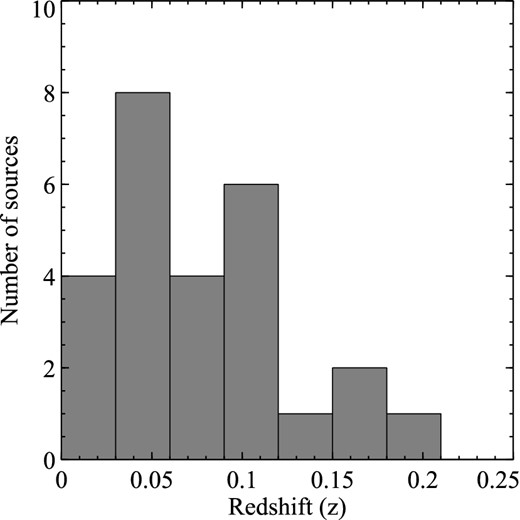
Distribution of the cosmological redshifts of the sources in the radio-loud AGN sample.
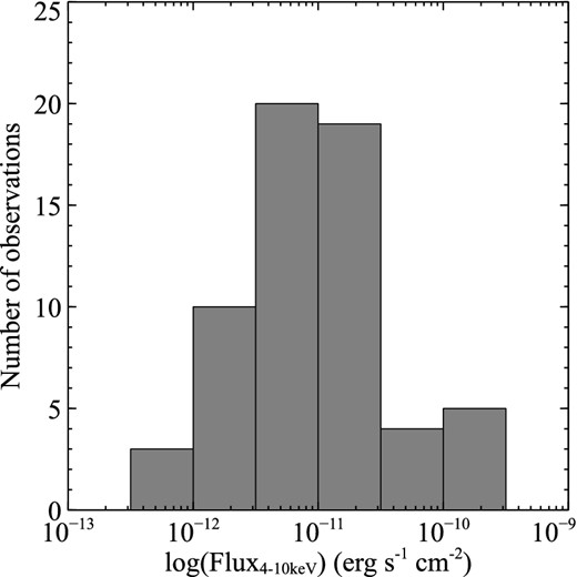
Distribution of the observed flux in the E = 4–10 keV energy band for the observations of the radio-loud AGN sample.
This sample of radio-loud AGN is directly complementary to that of Tombesi et al. (2010b), which focused on a search for UFOs in 42 local radio-quiet AGN (i.e. Seyferts) observed with XMM–Newton. A detailed comparison with respect to the sample of radio-quiet AGN of Tombesi et al. (2010b) will be presented in a subsequent paper (Tombesi et al., in preparation). Another recent systematic search for UFOs using Suzaku observations was reported by Gofford et al. (2013). In this case the authors selected a heterogeneous flux-based sample, considering spectra having >50.000 counts in the 2–10 keV band and both low-/high-redshift radio-quiet and radio-loud AGN, in particular 34 Seyferts, five quasars and six BLRGs. As discussed in Gofford et al. (2013), the results from the two XMM–Newton and Suzaku samples are formally consistent, with the Suzaku results suggesting that strong fast outflows also appear to be present at high luminosities/redshift (e.g. PDS 456 and APM 08279+5255), indicating that such winds may play an important role also near the peak of quasar growth/feedback at z ∼ 2.
2.1 XMM–Newton
We reduced the XMM–Newton observations using the standard procedures and the latest calibration data base. The data reduction was performed using the sas version 12.0.1 and the heasoft package version 6.12. We consider only the European Photon Imaging Camera-pn (EPIC-pn) instrument, which offers the highest sensitivity in the Fe K band between E = 3.5 and 10.5 keV. We checked for high background flare intervals and excluded these periods from the successive spectral analysis. The exposure time for the EPIC-pn spectra reported in Table B1 in Appendix B is net of the high background flare periods and detector dead time.
The majority of the observations did not show pile-up problems and the source and background regions were extracted from circles with 40 arcsec radii. However, there are some observations with significant pile-up, which required the source extraction region to be an annulus in order to exclude the inner part of the point spread function (PSF), which is more affected by this problem. The outer radius of the source and background regions in these cases was of 50 arcsec. Instead, the inner radius of the source annulus which was excluded from the analysis was of 5 arcsec for Pictor A (observation number 11 in Table B1 in Appendix B), 10 arcsec for PKS 0558−504 (observations 2b and 2c) and 20 arcsec for Centaurus A (observations 26a and 26b), respectively. The parameters of the XMM–Newton observations are listed in Table B1 in Appendix B.
2.2 Suzaku
The Suzaku data were reduced starting from the unfiltered event files and then screened applying the standard selection criteria described in the Suzaku ABC guide.2 We follow the same method outlined in Tazaki et al. (2013). The source spectra were extracted from circular regions of 3 arcmin radius centred on the source, whereas background spectra were extracted from a region of same size offset from the main target and avoiding the calibration sources. We generate the redistribution matrix file (rmf) and ancillary response file (arf) of the X-ray Imaging Spectrometer (XIS) with the xisrmfgen and xissimarfgenftools (Ishisaki et al. 2007), respectively. The spectra were inspected for possible pile-up contamination and this was corrected when present. The spectra of the front illuminated XIS-FI instruments (XIS 0, XIS 3 and also XIS 2 when available) were merged after checking that their fluxes were consistent. Instead, the data of the back illuminated XIS-BI instrument, the XIS 1, are not used due to the much lower sensitivity in the Fe K band and the possible cross-calibration uncertainties with the XIS-FI.
For the purpose of the broad-band spectral analysis, we also reduced the Suzaku PIN data for those sources showing possible absorption features in the Fe K band. The PIN data reduction and analysis was performed following the standard procedures. The source and background spectra were extracted within the common good time intervals and the source spectrum was corrected for the detector dead time. The ‘tuned’ non-X-ray background (NXB) event files provided by the Hard X-ray Detector (HXD) team are utilized for the background subtraction of the PIN data. The simulated cosmic X-ray background (CXB) is added to the NXB spectrum based on the formula given by Gruber et al. (1999). The PIN response file relative to each observation is used. We do not consider the Suzaku GSO data given the limited sensitivity of this instrument for the study of these sources. The parameters of the Suzaku observations are listed in Table B1 in Appendix B.
3 INITIAL FE K BAND SPECTRAL ANALYSIS
In this section we describe the initial spectra fitting of the data focused in the energy range E = 3.5–10.5 keV, i.e. the Fe K band. The different XMM–Newton EPIC-pn and Suzaku XIS spectra were grouped to a minimum of 25 counts for each energy bin in order to enable the use of the χ2 statistics when performing the spectral fitting. As already discussed in Tombesi et al. (2011b) and Gofford et al. (2013), equivalent results are obtained grouping to a slightly higher number of counts per bin and using of the χ2 statistic, not grouping the data at all and using the C-statistic (Cash 1979), or alternatively grouping the data to 1/5 of the full width at half-maximum (FWHM) of the instrument to sample the intrinsic energy resolution of the detector. The spectral analysis was carried out using the xspec v. 12.7.1 software. As pointed out in Table B1 in Appendix B, we do not analyse again those observations of 3C 111 (6), 3C 120 (4), 3C 382 (1), 3C 390.3 (1), 3C 445 (1) and 4C+74.26 (1) for which a detailed spectral analysis and search for Fe K absorbers was already reported in the literature using methods equivalent to the one employed here (e.g. Sambruna et al. 2009, 2011; Tombesi et al. 2010a,b, 2011a,b; Ballo et al. 2011; Braito et al. 2011; Gofford et al. 2013).
The analysis of the remaining 47 spectra was carried out in a homogeneous manner following a series of steps. Each spectrum was analysed in the E = 3.5–10.5 keV band using a baseline model similar to Tombesi et al. (2010a,b), i.e. a Galactic absorbed power-law continuum with possible narrow Gaussian Fe K emission lines. When required, we considered also additional neutral absorption intrinsic to the source. At this stage of the spectral analysis we did not include any Gaussian absorption lines but only emission lines when required. Throughout the analysis we consider only spectral components required at >99 per cent with the F-test. This baseline model provides a good representation of all the spectra in this restricted energy band. The best-fitting parameters for each observation are listed in Table A2 in Appendix A. Throughout this work the error bars refer to the 1σ level, if not otherwise stated.
Energy–intensity contour plots were calculated following the procedure described in Tombesi et al. (2010a,b). This consists in the fitting the spectrum with the previously derived baseline model without the inclusion of any absorption line and then stepping an additional narrow Gaussian line at intervals of 50 eV in the rest-frame energy interval between 5 and 10 keV with normalization free to be positive or negative. Each time the new χ2 is stored. In this way we derive a grid of χ2 values for different line energies and normalizations and then calculated the contours with the same Δχ2 level relative to the baseline model fit. We use Δχ2 levels of −2.3, −4.61 and −9.21, which correspond to F-test confidence levels for the addition of two more parameters of 68, 90 and 99 per cent, respectively. Because of the relatively high cosmological redshift (z = 0.1522) and the possible presence of absorption lines at high energies, the contour plots of PKS 1549−79 were calculated in the interval E = 5–12 keV for clarity. The ratio of the spectra with respect to the absorbed power-law continuum (without the inclusion of any Gaussian emission lines) and the contour plots with respect to the best-fitting baseline models (including Gaussian emission lines) are reported in Fig. C1 in Appendix C.
The contour plots were inspected for the possible presence of absorption features. The data analysis of a particular observation was interrupted if the contour plots showed no evidence for absorption features at rest-frame energies E > 6 keV with a significance at least >99 per cent, indicated by the blue contours in Fig. C1 in Appendix C.
The background counts are on average of the order or less than 2 per cent of the source ones in the 4–10 keV. However, it is important to note that both the EPIC-pn onboard XMM–Newton and the XIS cameras onboard Suzaku have an intense instrumental background emission line due to Cu Kα at E = 8.05 keV and Ni Kα at E = 7.48 keV, respectively (Katayama et al. 2004; Yamaguchi et al. 2006; Carter & Read 2007). These lines originate from the interaction of the cosmic rays with the sensor housing and electronics and this also causes their intensity to be slightly dependent on the location on the detector. Therefore, the selection of the background on a region of the CCD where the intensity of the lines is higher than that on the source extraction region can possibly induce spurious absorption lines in the background subtracted spectrum. If an indication of possible absorption lines was present in the contour plots, we then performed several checks to exclude the possibility that they were induced by an inadequate subtraction of instrumental background emission lines.
First, since the background emission lines are present at specific energies, we checked that the observed energies of the absorption lines are not consistent with those values. Secondly, we checked if the absorption lines were still present in the contour plots even without background subtraction. Only in two cases we find that the absorption lines could be induced by the background emission lines, namely 3C 206 and PKS 0707−35 (observations number 8 and 14 in Table A2 in Appendix A, respectively). Therefore, these two cases are excluded from the successive analysis.
From this initial study focused in the E = 3.5–10.5 keV band we find possible significant Fe K absorption lines at E > 6 keV in the contour plots of eight observations of five sources, namely 4C+74.26 (observations 1a and 1c), 3C 120 (observation 9f), PKS 1549−79 (observation 12a), 3C 105 (observation 16) and Centaurus A (observations 26c, 26d and 26e). In the next section and in Appendix A we investigate these observations in more detail. In particular, we derive a more robust detection of the possible absorption lines and reduce the uncertainties on the continuum level extending the analysis to the relative XMM–Newton and Suzaku broad-band spectra.
4 BROAD-BAND SPECTRAL ANALYSIS
In order to derive a more robust detection of the possible Fe K absorption lines and reduce the uncertainties on the continuum level, we then exploited the full broad-band capabilities of XMM–Newton EPIC-pn in the E = 0.5–10.5 keV and Suzaku in the E = 0.6–70 keV combining the XIS-FI (E = 0.6–10.5 keV, but excluding the interval between E = 1.5 and 2 keV due to calibration uncertainties) and PIN (E = 14–70 keV). We perform a broad-band spectral analysis only of the eight observations of five sources showing possible absorption lines in the contour plots in Fig. C1 in Appendix C, namely 4C+74.26 (observations 1a and 1c), 3C 120 (observation 9f), PKS 1549−79 (observation 12a), 3C 105 (observation 16) and Centaurus A (observations 26c, 26d and 26e).
The data analysis has been performed following a homogeneous standard procedure for all the observations. We start the broad-band analysis using a simple baseline model composed of a Galactic and intrinsically absorbed power-law continuum. Then, we inspect the residuals and include additional components that are required at more than the 99 per cent level. If required, for type 2 sources we include also a scattered continuum component in the soft X-rays with slope tied to the main continuum. The neutral Fe K emission lines previously modelled with Gaussians in the E = 3.5–10.5 keV analysis are now parametrized with a cold reflection component pexmon in xspec (Nandra et al. 2007), which takes simultaneously into account the neutral E = 6.4 keV Fe Kα fluorescent emission line, the relative Fe Kβ at E = 7.06 keV, the E = 7.45 keV Ni Kα and the high energy reflection hump. In this model we assume standard solar abundances, a high energy cut-off at E = 300 keV (e.g. Dadina 2007) and an inclination of 30° or 60° for type 1 and type 2 sources, respectively.
In a few cases we find that the spectra show some deviations from this standard baseline model. In particular, for 4C+74.26 we included two lowly ionized, soft X-ray warm absorber components modelled with two xstar tables with turbulent velocity of 100 km s−1. For the first observation (1a) of this source, the Fe K emission line detected at E ≃ 6.5 keV required also a mildly ionized reflection component modelled with a xillver table (García & Kallman 2010; García et al. 2013, 2014) instead of pexmon. The broad-band spectrum of Centaurus A requires a hot plasma emission component, apec in xspec, with temperature kT ≃ 0.65 keV to model the cluster/lobe emission in the soft X-rays and the neutral reflection component pexmon requires an iron abundance that is about 40 per cent of the solar value. The details of the fits for each observation are reported in the next sections.
Once a best fit was found, this broad-band model was used as a baseline to calculate the contour plots as discussed in Section 3 for the initial analysis focused in the Fe K band. The E = 5–10 keV contour plots were inspected again to check the presence of absorption feature(s) at rest-frame energies >6 keV with F-test significance >99 per cent. If the absorption line was confirmed, we modelled it with an inverted Gaussian and estimated the relative parameters, such as energy, width, intensity, EW and Δχ2 improvement to the fit.
In order to derive a more robust estimate of the detection significance for the absorption lines detected at E > 7 keV, we also performed 1000 Monte Carlo spectral simulations following the method outlined in Tombesi et al. (2010a,b). This allows us to better estimate the incidence of random fluctuations when considering lines in the relatively wide energy interval E = 7–10 keV. This usually provides a slightly lower significance than the standard F-test, which is applicable for a line observed at a certain expected energy, such as in the range E = 6.4–7 keV for K shell lines from neutral to hydrogen-like iron. Therefore, this test was required for those lines detected at rest-frame energies higher than 7 keV.
The Monte Carlo simulations allow us to test the null hypothesis that the spectra were adequately fitted by a model that did not include the absorption line. The analysis has been carried out as follows: (1) we simulated a spectrum (with the fakeit command in xspec) using the broad-band baseline model without any absorption line and considered the same exposure as the real data. We subtracted the appropriate background and grouped the spectrum to a minimum of 25 counts per energy bin; (2) this simulated spectrum was fitted with the baseline model and the resultant χ2 was stored; (3) then a narrow Gaussian line was added to the model, with its normalization initially set to zero and let free to vary between positive and negative values. In order to account for the possible range of energies in which the line could be detected, we then stepped its centroid energy between 7 and 10 keV at intervals of 100 eV, each time making a fit and stored only the maximum Δχ2; (4) this procedure was repeated 1000 times and consequently a distribution of simulated Δχ2 values was generated. This indicates the fraction of expected random generated emission/absorption features in the E = 7–10 keV energy band with a certain Δχ2 value. Thus, the Monte Carlo significance level of the observed line is represented by the ratio between the number of random lines with Δχ2 greater or equal to the real one with respect to the total number of simulated spectra. Following Tombesi et al. (2010a,b) and Gofford et al. (2013), we then select only the absorption features with a Monte Carlo confidence level higher than 95 per cent.
Finally, we perform a more physically self-consistent modelling of the absorption lines using the xstar tables and method described in Tombesi et al. (2011b). The nuclear X-ray ionizing continuum in the input energy range of xstar (E = 0.1 eV to E = 1 MeV) consists of a typical power-law continuum with photon index Γ = 2 and high energy cut-off at E > 100 keV. This is consistent with the average spectrum of local X-ray bright radio-quiet/radio-loud AGN (e.g. Kataoka et al. 2007; Sambruna, Reeves & Braito 2007; Dadina 2008; Sambruna et al. 2009, 2011; Ballo et al. 2011; Tombesi et al. 2011b, 2013b; Lohfink et al 2013; Tazaki et al. 2013). In fact, the jet contribution to the X-ray emission of the sources in our sample is found by Tazaki et al. (in preparation) to be negligible. We use standard solar abundances (Asplund et al. 2009) and tested three turbulent velocities of 1000, 3000 and 5000 km s−1.
The broad-band analysis of the eight observations of five sources (namely, 4C+74.26, 3C 120, PKS 1549−79, 3C 105 and Centaurus A) with detected Fe K absorption lines are described in detail in Appendix A. The best-fitting xstar parameters of their Fe K absorbers, along with those already reported in the literature for other radio-loud AGN of this sample, are listed in Table 1. In Appendix A we discuss the robustness of these results for each case, checking that they are not affected by the possible inclusion of rest-frame neutral or ionized partial covering absorption or disc reflection features. For the latter, this was also expected due to the already reported fact that reflection features are generally weak in radio galaxies (e.g. Ballantyne, Fabian & Iwasawa 2004; Kataoka et al. 2007; Larsson et al. 2008; Sambruna et al. 2009, 2011; Tombesi et al. 2011a, 2013b; Lohfink et al. 2013; Tazaki et al. 2013). We point to Tazaki et al. (in preparation) for a detailed description of the accretion disc and torus reflection features for most of the sources listed in Table B1.
Best-fitting xstar parameters of the Fe K absorbers from the broad-band spectral analysis and radio jet inclination for each source.
| Source | Num | log ξ | NH | vout | Δχ2/Δν | χ2/ν | PF | α |
|---|---|---|---|---|---|---|---|---|
| (1) | (2) | (3) | (4) | (5) | (6) | (7) | (8) | (9) |
| This work | ||||||||
| 4C+74.26 | 1a | 4.62 ± 0.25 | >4* | 0.045 ± 0.008 | 13.7/3 | 1451.1/1427 | 99.6 per cent | <49°f |
| 3C 120 | 9f | 4.91 ± 1.03 | >2* | 0.161 ± 0.006 | 15.3/3 | 2933.0/2540 | 99.5 per cent | 20| $_{.}^{\circ}$|5 ± 1| $_{.}^{\circ}$|8g |
| PKS 1549-79 | 12a | 4.91 ± 0.49 | >14 | 0.276 ± 0.006 | 25.0/4 | 850.0/930 | 99.99 per cent | <55°h |
| Tied | Tied | 0.427 ± 0.005 | ||||||
| 3C 105 | 16 | 3.81 ± 1.30 | >2* | 0.227 ± 0.033 | 10.5/3 | 226.4/253 | 99 per cent | >60° |
| Centaurus A | 26c | 4.33 ± 0.03 | 4.2 ± 0.4 | <0.004* | 126.5/2 | 2830.9/2682 | ≫99.99 per cent | 50°–80°i |
| 26d | 4.39 ± 0.06 | 4.1 ± 0.9 | <0.005* | 54.7/2 | 2852.2/2661 | ≫99.99 per cent | ||
| 26e | 4.31 ± 0.10 | 4.0 ± 1.1 | <0.003* | 105.3/2 | 2855.8/2698 | ≫99.99 per cent | ||
| From the literature | ||||||||
| 4C+74.26 | 1bc | 4.06 ± 0.45 | >0.6* | 0.185 ± 0.026 | ||||
| 3C 390.3 | 6ca | |$5.60^{+0.20}_{-0.80}$| | >3* | 0.146 ± 0.004 | 19°–33°j | |||
| 3C 111 | 7ba | 5.00 ± 0.30 | >20* | 0.041 ± 0.003 | 18| $_{.}^{\circ}$|1 ± 5| $_{.}^{\circ}$|1g | |||
| 7db | 4.32 ± 0.12 | 7.7 ± 2.9 | 0.106 ± 0.006 | |||||
| 3C 120 | 9c,d,ea | 3.80 ± 0.20 | |$1.1^{+0.5}_{-0.4}$| | 0.076 ± 0.003 | ||||
| 3C 445 | 18bd, e | |$1.42^{+0.13}_{-0.08}$| | |$18.5^{+0.6}_{-0.7}$| | 0.034 ± 0.001 | 60°–70°k | |||
Note: (1) Object name. (2) Observation number. (3) Logarithm of the ionization parameter in units of erg s−1 cm. (4) Column density in units of 1022 cm−2. (5) Outflow velocity in units of the speed of light, c. (6) χ2 improvements with respect to the additional parameters with respect to the baseline model. (7) Final best-fitting χ2 and degrees of freedom ν. (8) F-test confidence level. (9) Radio jet inclination angle. Given the lack of a reported value in the literature, we assume an inclination angle of α > 60° for 3C 105 given its optical classification as type 2.
*Upper or lower limit at the 90 per cent. aTombesi et al. (2010a), bTombesi et al. (2011a), cGofford et al. (2013), dBraito et al. (2011), eReeves et al. (2010), fPearson et al. (1992), gJorstad et al. (2005), hHolt et al. (2006), iTingay et al. (1998), jEracleous & Halpern (1998), kSambruna et al. (2007).
The observation number 1c of 4C+74.26 is the only case in which we find complexities in the Fe K band in the form of broad emission and absorption which could be modelled as disc reflection and a fast ionized outflow or as a rest-frame partial covering ionized absorber. This is discussed in Appendix A in Section A1.3. Given that we cannot strongly distinguish between these two models, we conservatively exclude the discussion of this particular observation from Table 1 and Section 5. This does not change the overall conclusions on the whole sample.
5 RESULTS
5.1 Incidence of UFOs in radio-loud AGN
Following the definition of UFOs as those highly ionized Fe K absorbers with outflow velocities higher than 10 000 km s−1 (Tombesi et al. 2010a,b), here we derive an estimate of the incidence of such absorbers in the sample of radio-loud AGN. If we consider only the spectra analysed in this work, we find that UFOs are detected in only 4/48 (≃8 per cent) of the observations or 4/25 (≃16 per cent) of the sources, respectively. Instead, if we include also all the observations of the sources in the sample that were already studied in detail in the literature, we find that UFOs are detected in a total of 12/61 (≃20 per cent) of the observations or 7/26 (≃27 per cent) of the sources, respectively.
It is important to note that these detection fractions can significantly underestimate the real values because they do not take into account the number of observations that have low counts levels and therefore do not have enough statistics for the detection of Fe K absorption lines even if present.
Following Tombesi et al. (2010b), the net 4–10 keV counts of each observation can be regarded as an indication of their statistics and we can estimate the number of counts required to obtain a reliable line detection. We can estimate the effect of the limited statistics available in the spectra of the whole sample considering a mean EW of 50 eV and a line energy of 8 keV, corresponding to a blueshifted velocity of about 0.1c for Fe xxvi Lyα (Tombesi et al. 2010b). These values are equivalent to the average EW and energy of the blueshifted Fe K absorption lines in radio-loud AGN reported here and in the literature of 〈EW〉 ≃ 45 eV and 〈E〉 ≃ 8.2 keV. The 4–10 keV counts level needed for a 3σ detection of such a line is ≃104 and ≃2 × 10⁴ counts for the EPIC-pn instrument onboard XMM–Newton and the combined XIS front illuminated CCDs of Suzaku, respectively. This criterion is met by 15 XMM–Newton and 19 Suzaku observations, respectively. Therefore, as we can see from the cumulative distributions of counts in Fig. 3, only about 56 per cent of the available XMM–Newton and Suzaku observations have enough counts for a proper detection of highly ionized UFOs with a typical velocity of ∼0.1c.
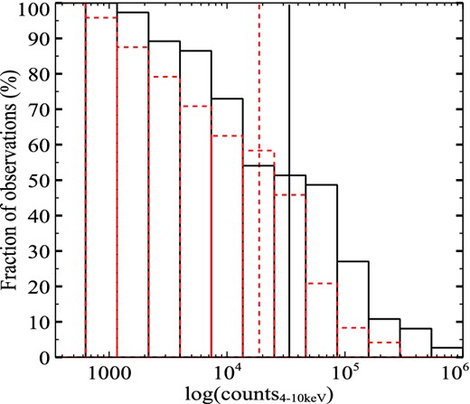
Cumulative distributions of the net 4–10 keV counts of the XMM–Newton (red dashed lines) and Suzaku (black solid lines) observations. The vertical lines refer to the values of 104 counts (red dashed) and 2 × 10⁴ counts (black solid). These values correspond to the counts levels required for a significant detection of a typical UFO absorption line in the XMM–Newton and Suzaku spectra, respectively.
This test demonstrates that the comparison of UFO detections with respect to the total number of observations or sources can drastically underestimate the actual fraction because this does not take into account the fact that several observations can have insufficient counts. Therefore, considering only the observations with enough counts we have a UFO detection fraction of 12/34 (≃32 per cent), which corresponds to an incidence of 6/12 (≃50 per cent) for this subsample of sources.
However, if we want to extrapolate this fraction to the whole sample, we have to take into account our ignorance due to the number of sources with low signal-to-noise ratio (S/N) observations. Assuming that a UFO is present in either none or all of the sources with low S/N we can estimate the lower and upper limits corresponding to 7/26 (≃30 per cent) and 20/26 (≃70 per cent), respectively. Therefore, the incidence of UFOs in our sample of radio-loud AGN can be estimated to be in the range f ≃ (50 ± 20) per cent. Interestingly, this is consistent with what reported for similar studies of large samples of radio-quiet AGN (Tombesi et al. 2010b; Patrick et al. 2012; Gofford et al. 2013).
For the sources optically classified as type 1 or type 2 we have a detection fraction of 5/12 (≃42 per cent) and 1/12 (≃8 per cent), respectively. However, taking into account that the sources having spectra with enough counts are only 10 for type 1s and 2 for type 2s, the most likely fractions can be estimated to be 5/10 and 1/2, respectively. This translates in an incidence of UFOs of ∼50 per cent for both type 1s and type 2s. However, these values are only indicative, given the small number statistics, especially for type 2s.
The Monte Carlo simulations discussed in Section 4 ensure that the reported blueshifted absorption lines indicative of UFOs are detected at a confidence level >95 per cent against random positive and negative fluctuations in the wide energy band between E = 7 and 10 keV. Therefore, we would naively expect to have a random emission or absorption line in the interval E = 7–10 keV in one spectrum out of 20. Considering all the 61 observations, the maximum fraction of random detections would be ∼3. Moreover, considering that there are only 34 observations with enough S/N to detect a typical UFO if present, this would results in a maximum of ∼1–2 random lines. These estimates are much lower than 12, the number of actual spectra with at least one highly blueshifted absorption line detected.
As already noted by Tombesi et al. (2010b) and Gofford et al. (2013), a more quantitative estimate of the global probability that the observed absorption features are purely due to statistical noise can be derived using the binomial distribution. Given that there are n = 12 spectra with at least one blueshifted absorption line detected with a Monte Carlo probability ≥95 per cent out of a total of N = 61, the probability of one of these lines to be due to random noise is p < 0.05. Therefore, their global random probability is P < 3 × 10⁻⁵ and therefore the confidence level is >99.997 per cent (>4σ). However, considering that only N = 34 spectra have enough S/N, the global random probability would further decrease to P < 4 × 10⁻⁸ (>5.5σ).
From Table B1 in Appendix B we see that of the 23 sources with a Fanaroff & Riley classification, 20 are identified as FR IIs and only three as FR Is. As discussed in Section 2, the paucity of FR Is can be explained as a selection effect due to the fact that we consider an X-ray selected flux-limited sample and they have a systematically lower luminosity than FR IIs (e.g. Fabbiano et al. 1984; Hardcastle et al. 2009). Comparing with Table 1, we see that 6/20 (∼30 per cent) of FR IIs and 1/3 (∼30 per cent) of FR Is have outflows with observed velocities higher than 10 000 km −1, identified as UFOs, and only 1/3 of FR Is (Centaurus A) has an Fe K absorber with an observed low velocity of ≲ 1000 km s−1. However, if we limit only to the number of sources having at least one observation with enough S/N to detect UFOs if present, we find that 5/10 (∼50 per cent) of FR IIs and 1/2 (∼50 per cent) of FR Is show UFOs and 1/2 of FR Is (Centaurus A) show an Fe K absorber with an observed low velocity of ≲ 1000 km s−1. The very limited number of FR Is compared to FR IIs in this sample (3/20) does not allow us to perform a significant comparison between these two populations.
Finally, we note that the majority of the sources are classified as FR II (20) and only a few as FR I (3). Moreover, in the definition of the sample we specifically excluded those sources classified as blazars. Therefore, the estimate of the incidence of UFOs in radio-loud AGN should be considered within the limit of this sample.
5.2 Parameters of the Fe K absorbers in radio-loud AGN
The distributions of the xstar parameters of the Fe K absorbers detected in the radio-loud AGN sample are reported in Fig. 4. These values include also those sources with equivalent studies already reported in the literature and listed in Table 1.
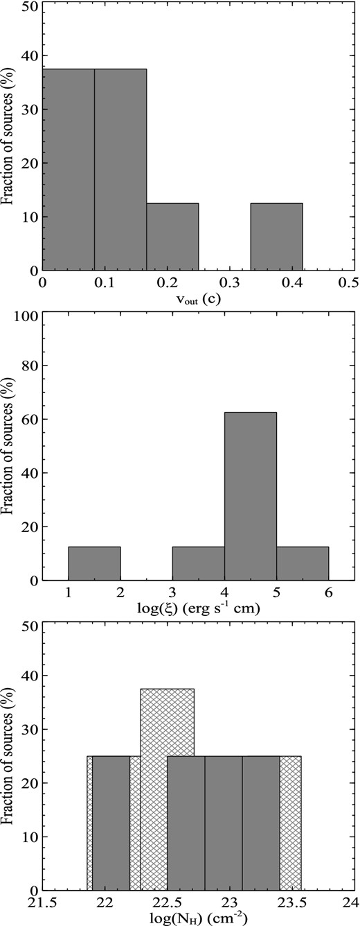
Distributions of mean Fe K absorber parameters for each source in the radio-loud AGN sample: logarithm of the mean outflow velocity (upper panel), logarithm of the mean ionization parameter (middle panel) and logarithm of the mean column density (lower panel). In the lower panel, the histogram derived using all the values including lower limits is indicated with diagonal crosses, instead the one derived using the measured values is in grey.
The upper panel of Fig. 4 shows the distribution of the average outflow velocity of the Fe K absorbers detected for each source. The values are broadly distributed between vout ≲ 1000 km −1 (for Centaurus A) and vout ≃ 0.4c. All the outflows, excluding only Centaurus A, have velocities higher than 10 000 km s−1 and can be directly identified with UFOs. In general, the Fe K absorbers have mildly relativistic mean and median velocities of vout ≃ 0.133c (vout ≃ 0.152c without Centaurus A) and vout ≃ 0.117c (vout ≃ 0.119c without Centaurus A), respectively.
As already discussed in Tombesi et al. (2011b), this velocity distribution has a bias that hampers the detection of outflows with high velocities. This is due to the fact that the sensitivity of the XMM–Newton and Suzaku CCDs quickly drops at energies higher than E ≃ 8–9 keV and therefore outflows with velocities higher than vout ∼ 0.3–0.4c would be impossible to detect for these local sources. For instance, UFOs with even higher velocities have been reported for a few bright quasars at much higher cosmological redshifts (e.g. Chartas et al. 2002, 2003, 2009; Lanzuisi et al. 2012). Moreover, these outflow velocities are only conservative estimates because they represent the projected wind velocity along the line of sight and therefore they depend on the inclination of the source and the wind with respect to the observer.
The distribution of the ionization parameter shown in the middle panel of Fig. 4 has mean and median values of log ξ ≃ 4.18 erg s−1 cm (log ξ ≃ 4.57 erg s−1 cm without 3C 445) and log ξ ≃ 4.35 erg s−1 cm (log ξ ≃ 4.36 erg s−1 cm without 3C 445), respectively. This is consistent with the fact that the material is usually observed through highly ionized Fe xxv–xxvi absorption lines. However, we note the presence of an outlier at log ξ ≃ 1.5 erg s−1 cm due to 3C 445. As already discussed in Reeves et al. (2010) and Braito et al. (2011) this could be due to the fact that we are observing the wind in this source with a high inclination or the wind geometry is mainly equatorial. Indeed, this picture is consistent with the high inclination of its radio jet (Eracleous & Halpern 1998; Sambruna et al. 2007) and the expectation of increasing/decreasing column density/ionization of accretion disc winds moving from low to high inclination angles (e.g. Proga & Kallman 2004; Fukumura et al. 2010).
The distribution of the average observed column density of the Fe K absorbers for each source listed in Table 1 is shown in the lower panel of Fig. 4. This is distributed in the range between log NH ≃ 22 and ≃23.5 cm−2. Considering only the values constrained within the errors (reported in grey), the mean and median values are log NH = 22.7 and 22.75 cm−2, respectively. Instead, considering all the values including the lower limits (showed as diagonal crosses) the mean and median values of the column densities are NH > 22.66 and >22.55 cm−2, respectively.
We note that the parameters of the Fe K absorbers of the radio-loud AGN sample shown in Fig. 4 are broadly consistent with those reported by similar other studies focused on radio-quiet sources (Tombesi et al. 2010b; Gofford et al. 2013). A detailed comparison with the Fe K absorbers detected in radio-quiet AGN will be discussed in a subsequent paper (Tombesi et al., in preparation).
5.3 Variability of the Fe K absorbers
As we can see from Table 1, there are three sources with multiple detections of UFOs in different observations. In 4C+74.26 the UFO is possibly detected in all the three observations taken, respectively, in 2004 June, 2007 October and 2011 November. However, we conservatively do not consider the last observation due to some modelling ambiguities. Comparing the first two observations, the ionization levels and column densities are consistent within the errors but the velocity changed on a time-scale of about 3 yr.
The BLRG 3C 111 was observed five times with XMM–Newton and Suzaku, with the UFO being significantly detected twice. The intervals between these observations are ∼6 months, ∼2 yr and 1 week. Including an xstar table with the typical velocity of vout ≃ 0.1c and ionization parameter of log ξ ≃ 4.5 erg s−1 cm for the UFOs from Fig. 4 we can estimate the 90 per cent upper limits on the column density for the observations without a significant UFO detections. We obtain NH < 4 × 1022 cm−2 for 7a, NH < 8 × 1022 cm−2 for 7c and NH < 6 × 1022 cm−2 for 7e, respectively. Given the limited statistics, the column density can only be constrained to be variable on time-scales of less than ∼6 months and ∼2 yr between observations 7a–7b and 7b–7c, respectively. However, considering the EW of the relative absorption line, the UFO is inferred to be variable on time-scales down to about 1 week (Tombesi et al. 2011a). Considering only the two observations with clear detections, the UFO is found to vary in both column density and velocity at the 90 per cent level on time-scales of less than ∼2 yr.
The radio galaxy 3C 120 was observed for a total of seven times, however, three Suzaku observations taken within 2 weeks were merged to increase their statistics (Tombesi et al. 2010a) and therefore only five spectra were analysed. The intervals between these observations are ∼3.5 yr, ∼2 weeks, ∼6 yr and ∼1 week. Including an xstar table with typical UFO parameters, as already done previously for 3C 111, we can estimate the 90 per cent upper limits on the column density for the observations without a significant UFO detections. We obtain NH < 3 × 1022 cm−2 for 9a, NH < 2 × 1022 cm−2 for 9b and NH < 5 × 1022 cm−2 for 9g, respectively. Given the limited statistics and the possible intrinsic weakness of the UFO in this source, the variability of the column density can only be roughly estimated to be on time-scales shorter than 6 yr comparing the two detections. Also the outflow velocity is variable on these time-scales. However, we note that the detection of the first outflow was not unambiguously confirmed in a broad-band Suzaku spectral analysis using different models by Gofford et al. (2013).
The galaxy 3C 390.3 was observed three times, at intervals of ∼9 d and ∼2 yr. The UFO was significantly detected in the last long Suzaku observations. Also in this case, including an xstar table with typical UFO parameters we can estimate the 90 per cent upper limits on the column density for the observations without a significant UFO detections. We obtain NH < 7 × 1022 cm−2 for 6a and NH < 5 × 1022 cm−2 for 6b, respectively. Given the limited statistics, the variability of the column density cannot be constrained, as the upper and lower limits are consistent between all three observations.
PKS 1549−79 was also observed twice, with XMM–Newton and Suzaku, with an interval between the two of about 1 month. Two Fe K absorption lines indicating a complex UFO with at least two velocity components of ≃0.276c and ≃0.427c was significantly observed in the first XMM–Newton observation. However, their presence cannot be excluded in the Suzaku observation at the 90 per cent level. In particular, an absorption line at the same energy of E ≃ 11 keV and consistent EW as in the XMM–Newton spectrum is also independently detected in Suzaku, although at a lower significance of ∼92 per cent which falls below our detection threshold. Finally, 3C 105 was observed only once with Suzaku and the UFO was observed in this observation. The lack of additional observations of this source does not allow its variability to be investigated.
Regarding the detection of the Fe K absorber with low observed velocity of ≲ 1000 km s−1 in Centaurus A, this has been clearly detected in three long Suzaku observations taken within a period of 1 month in 2009. The values of the ionization and column density are consistent within the errors, indicating that the absorber did not vary on this relatively short time-scale. However, there was no significant detection of Fe K absorption lines in the XMM–Newton observations taken in 2001 and 2002. Therefore, the absorber can indeed be variable at least on time-scales of less than ∼7 yr.
5.4 Comparison with the radio jet inclination
In Table 1 we report the estimates of the inclination angle of the radio jet with respect to the line of sight for the sources with detected Fe K absorbers. Assuming that the jet is perpendicular to the accretion disc, this would represent also the angle with which we are looking at the accretion disc. Considering only the UFOs (i.e. excluding Centaurus A), we note that the inclination angle spans a wide range of values from ∼10° to ∼70°, indicating that these winds have a large opening angle and that they are not preferentially equatorial. This is consistent with the high covering fraction derived from the incidence of UFOs in the sample of ∼0.3–0.7.
In Fig. 5 we show a comparison between the jet inclination angle and the average column density, ionization parameter and outflow velocity of the UFOs for each source with a detection. Given the large uncertainties (mostly lower limits) on the column densities, we do not see any clear trend between log NH and jet inclination. Instead, the data are suggestive of a possible trend of decreasing ionization parameter and increasing outflow velocity going from low to intermediate or high inclination angles. However, we note that given the large uncertainties on the jet angles and the presently unknown angle between the jet and the wind, these plots should be considered only as illustrative.
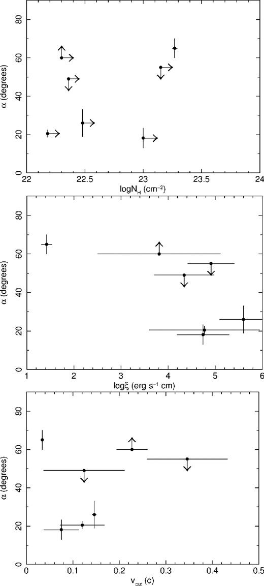
Comparison between the inclination of the radio jet and the average column density (upper panel), ionization parameter (middle panel) and outflow velocity (lower panel) of the UFOs for each source.
6 DISCUSSION
Combining the results of this analysis with those in the literature we find that UFOs are detected in >27 per cent of the sources. However, correcting for the number of spectra with insufficient S/N, we can estimate that the incidence of UFOs is likely in the range f ≃ (50 ± 20) per cent. From the fraction of radio-loud AGN with detected UFOs and assuming a steady wind, we can roughly infer an estimate of the minimum covering fraction of C = Ω/4π ≃ 0.3–0.7, where Ω is the solid angle subtended by the wind with respect to the X-ray source. Thus, as an ensemble, the UFOs in radio-loud AGN might cover a significant fraction of the sky as seen by the central X-ray source. This also provides an important geometric constraint indicating that the distribution of the absorbing material is not very collimated as in jets, thereby implying large opening angles. The UFOs are detected for sources with jet inclination angles in the wide range from ∼10° to ∼70°. This further supports the idea that these winds have indeed a large opening angle and are not preferentially equatorial.
Interestingly, the detection fraction of UFOs is similar to that reported for complementary studies of large samples of radio-quiet AGN (Tombesi et al. 2010b; Patrick et al. 2012; Gofford et al. 2013). This is also comparable to that of the slower and less ionized warm absorbers detected in the X-ray spectra of Seyfert 1 galaxies (Reynolds 1997; George et al. 1998; Blustin et al. 2005; McKernan, Yaqoob & Reynolds 2007; Tombesi et al. 2013a). In particular, warm absorbers have been reported in some X-ray bright BLRGs as well (Reynolds 1997; Ballantyne 2005; Reeves et al. 2009b, 2010; Torresi et al. 2010, 2012; Braito et al. 2011).
The fact that UFOs are observed in a similar fraction of both radio-loud and radio-quiet AGN suggests that this dichotomy, which differentiates sources with and without strong radio jets, might actually not hold for UFOs or AGN winds in general. This would actually be expected from the fact that AGN winds should depend mainly, if not only, on the state of the accretion disc and not, for instance, on the black hole spin, as for relativistic jets (e.g. Blandford & Znajek 1977; Tchekhovskoy, Narayan & McKinney 2010; Tchekhovskoy et al. 2011; Tchekhovskoy & McKinney 2012). For instance, from a theoretical point of view, winds/outflows are ubiquitous in both cold, thin accretion discs and hot, think accretion flows and they can be driven by several mechanisms, such as thermal, radiative or MHD (e.g. Blandford & Payne 1982; Blandford & Begelman 1999; King & Pounds 2003; Proga & Kallman 2004; McKinney 2006; Ohsuga et al. 2009; Fukumura et al. 2010, 2014; Tchekhovskoy et al. 2011; Yuan, Bu & Wu 2012; Sa̧dowski et al. 2013, 2014).
A statistically significant study of the variability of the UFOs is hampered by the limited number of sources with multiple observations and by their inhomogeneous monitorings. In fact, the variability study of the parameters of the UFOs was possible only for the five sources with more than one observation. In particular, 3/5 sources have multiple detections of UFOs. Combining the values derived in this study and those collected from the literature in Table 1, we find that the velocity is significantly variable in 3/3 cases, NH in 2/3 cases and log ξ in 1/3 cases. Comparing also the observations with and without detections, we find that UFOs can be variable even on time-scales as short as a few days. This is consistent with the idea that these absorbers are preferentially observed at ∼subpc scales from the central SMBH in radio-loud AGN and that they may also be intermittent, possibly being stronger during jet ejection or outburst events on longer time-scales of the order of half to one year (Tombesi et al. 2011a, 2012b, 2013b).
Overall, the characteristics of these UFOs – high ionization levels, column densities, variability and often mildly relativistic velocities – are qualitatively in agreement with the picture of complex AGN accretion disc winds inferred from detailed simulations (e.g. Ohsuga et al. 2009; Fukumura et al. 2010; King 2010; Takeuchi, Ohsuga & Mineshige 2014). Indeed, the reported limits on the location of the UFOs in a few radio-loud AGN indicate that they are at distances of ∼100–10 000rs from the SMBH, therefore, at accretion disc scales (e.g. Reeves et al. 2010; Tombesi et al. 2010a, 2011a, 2012b). However, a homogeneous and systematic estimate of the location, mass outflow rate and energetics of the UFOs in this sample, along with a comparison with those detected in radio-quiet AGN, will be discussed in a subsequent paper (Tombesi et al., in preparation). This will allow us to perform a more detailed discussion of the validity of the jet related radio-quiet/radio-loud dichotomy for winds and possibly to better constrain their acceleration mechanisms and energetics (e.g. King & Pounds 2003; Everett & Ballantyne 2004; Proga & Kallman 2004; Everett 2005; Ohsuga et al. 2009; Fukumura et al. 2010, 2014; Kazanas et al. 2012; Ramírez & Tombesi 2012; Reynolds 2012; Tombesi et al. 2013a).
7 CONCLUSIONS
We performed a systematic and homogeneous search for Fe K absorption lines in the XMM–Newton and Suzaku spectra of a large sample of 26 radio-loud AGN selected from the Swift BAT catalogue. After an initial investigation of the E = 3.5–10.5 keV spectra we performed a more detailed broad-band analysis of eight observations of five sources showing possible Fe K absorption lines that were not already reported in the literature. The detection significance of these lines was further investigated through extensive Monte Carlo simulations and the parameters of the Fe K absorbers were derived using the xstar photoionization code.
Combining the results of this analysis with those in the literature we find that UFOs are detected in >27 per cent of the sources. However, correcting for the number of spectra with insufficient S/N, we can estimate that the incidence of UFOs is likely in the range f ≃ (50 ± 20) per cent. This value is comparable to that of UFOs and warm absorbers in radio-quiet AGN, suggesting that the jet related radio-quiet/radio-loud AGN dichotomy might not hold for AGN winds. However, we note that the majority of the sources in the present sample are classified as FR II (20) and only a few as FR I (3). Moreover, in the definition of the sample we specifically excluded those sources classified as blazars. Therefore, the estimate of the incidence of UFOs in radio-loud AGN should be considered within the limit of this sample.
From the xstar fits we derive a distribution of the main Fe K absorber parameters. The mean (vout ≃ 0.133c) and median (vout ≃ 0.117c) outflow velocities are mildly relativistic, but the observed values are broadly distributed between vout ≲ 1000 km s−1 (for the highly inclined radio galaxy Centaurus A) and vout ≃ 0.4c. The ionization of the material is high, with an average value of log ξ ≃ 4.5 erg s−1 cm, and the lines are consistent with resonance absorption from Fe xxv–xxvi. Finally, the column densities are larger than log NH > 22 cm−2.
The UFOs are detected for sources with jet inclination angles in the wide range from ∼10° to ∼70°. This further supports the idea that these winds have a large opening angle and are not preferentially equatorial. Overall, these characteristics are consistent with the presence of complex accretion disc winds in a significant fraction of radio-loud AGN. A detailed comparison with the Fe K absorbers detected in radio-quiet AGN is discussed in a subsequent paper (Tombesi et al., in preparation). Finally, important improvements in these studies are expected from the upcoming ASTRO-H (Takahashi et al. 2012) and the future Advanced Telescope for High ENergy Astrophysics (ATHENA) observatories (Cappi et al. 2013; Nandra et al. 2013).
FT would like to thank R. M. Sambruna for her contribution to the initial definition of the project and for the comments to the manuscript. FT thanks C. S. Reynolds and G. M. Madejski for the useful discussions. FT acknowledges support for this work by the National Aeronautics and Space Administration (NASA) under Grant No. NNX12AH40G issued through the Astrophysics Data Analysis Program, part of the ROSES 2010.
REFERENCES
APPENDIX A: BROAD-BAND SPECTRAL ANALYSIS OF THE SOURCES WITH ABSORPTION LINES
A1 4C+74.26
A1.1 Observation 1a
We analysed the XMM–Newton EPIC-pn spectrum of 4C+74.26 (observation number 1a) considering the observed energy range between E = 0.5 and 10.5 keV. The best-fitting model comprises a neutral absorbed power-law continuum with Γ = 1.74 ± 0.01 and column density NH = (5 ± 1) × 1020 cm−2. The neutral absorption component is required at ≫99.99 per cent using the F-test.
The energy of the Fe Kα emission line of E = 6.50 ± 0.04 keV reported in Table B2 in Appendix B suggests that the reflection should come from mildly ionized material instead of neutral material expected at E = 6.4 keV. This evidence was already discussed in Ballantyne (2005) and Gofford et al. (2013). Indeed, the inclusion of an ionized reflection component modelled with xillver (García & Kallman 2010; García et al. 2013, 2014) provides a very significant fit improvement of Δχ2/Δν = 35/1 with respect to that using a neutral pexmon component. The resultant ionization parameter is |$\xi = 300^{+53}_{-46}$| erg s−1 cm.
As already reported in Ballantyne (2005) and Gofford et al. (2013), the soft X-ray spectrum of 4C+74.26 shows intense O vii and O viii absorption edges indicative of ionized material along the line of sight. These features are well parametrized with the inclusion of two warm absorber components. Therefore, we use two xstar tables with a typical Γ = 2 ionizing continuum and turbulent velocity of 100 km s−1. Given the relatively low energy resolution of the EPIC-pn spectrum in the soft X-rays, we cannot reliably constrain their possible velocity shifts, which were fixed to zero. The fit improvement after including these two ionized warm absorbers is very high, Δχ2/Δν = 476.2/4, indicating a confidence level of ≫99.99 per cent.
The fit improvement after the inclusion of a Gaussian absorption line at the rest-frame energy of E = 7.28 ± 0.05 keV is Δχ2/Δν = 13.0/2, corresponding to an F-test probability of 99.8 per cent. Given that the energy of the line is not directly consistent with that expected from ionized iron at rest, we also performed Monte Carlo simulations in order to better estimate its detection level as described in Section 4. The resultant Monte Carlo probability is 99.2 per cent, which is higher than the selection threshold of 95 per cent. The final model provides a very good representation of the data, as shown in Fig. A1. Instead, the contour plot in the E = 5–10 keV energy band with respect to the baseline model without the inclusion of the absorption line is reported in Fig. A2. The best-fitting parameters are listed in Table A1.
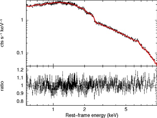
Broad-band XMM–Newton EPIC-pn spectrum and ratios against the best-fitting model (red) of 4C+74.26 (number 1a) in the E = 0.5–10 keV energy band.
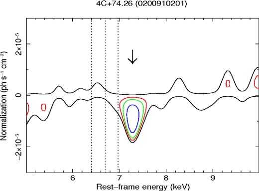
Energy–intensity contour plot in the interval E = 5–10 keV calculated using the broad-band spectrum of 4C+74.26 (number 1a), see text for more details. The arrow points the absorption line. The vertical lines refer to the energies of the neutral Fe Kα, Fe xxv and Fe xxvi lines at E = 6.4, 6.7 and 6.97 keV, respectively.
Best-fitting broad-band model of 4C+74.26 (number 1a).
| Neutral absorption | |
| NH (1022 cm−2) | 0.05 ± 0.01 |
| Warm absorber 1 | |
| NH (1022 cm−2) | |$0.40^{+0.10}_{-0.06}$| |
| log ξ (erg s−1 cm) | |$2.53^{+0.04}_{-0.02}$| |
| z | 0.104 |
| Warm absorber 2 | |
| NH (1022 cm−2) | |$0.17^{+0.02}_{-0.03}$| |
| log ξ (erg s−1 cm) | |$1.06^{+0.04}_{-0.09}$| |
| z | 0.104 |
| Power-law continuum | |
| ΓPow | 1.74 ± 0.01 |
| Ionized reflection (xillver) | |
| ΓXil | ΓPow |
| ξ (erg s−1 cm) | |$300^{+53}_{-46}$| |
| N (10−7) | |$2.2^{+0.6}_{-0.4}$| |
| AFe (solar) | 1 |
| Absorption line | |
| E (keV) | 7.28 ± 0.05 |
| σ (eV) | 100 |
| I (10−5 photon s−1 cm−2) | −0.90 ± 0.20 |
| EW (eV) | −35 ± 8 |
| Absorption line statistics | |
| Δχ2/Δν | 13.0/2 |
| F-test (per cent) | 99.8 |
| MC (per cent) | 99.2 |
| Broad-band model statistics | |
| χ2/ν | 1451.9/1428 |
We checked the possible alternative phenomenological modelling of the broad absorption feature with a photoelectric edge. The inclusion of an edge provides a slightly higher fit improvement of Δχ2/Δν = 42.2/2. However, the resultant rest-frame energy of E = 7.12 ± 0.06 keV is consistent with neutral iron with a maximum optical depth of |$\tau = 0.097^{+0.013}_{-0.016}$|, which would indicate a large column density of NH ∼ 1023 cm−2. This is at odds with the fact that such neutral absorption component is not required when fitting the broad-band spectrum (Δχ2/Δν = 1.4/1), with a stringent upper limit on the column density of NH < 5 × 1020 cm−2. We also checked the possible identification of an ionized iron edge including another xstar component used for the modelling of the warm absorbers. The resultant fit improvement is negligible (Δχ2/Δν = 2.9/2). Therefore, even if the phenomenological modelling with a single edge provides a fit comparable to that of a broad Gaussian absorption line, this possibility is rejected because the data do not require any further neutral or lowly ionized absorption component.
If identified with Fe xxv Heα or Fe xxvi Lyα the broad absorption line would indicate a significant blueshifted velocity of ≃0.16–0.19c. If only due to a velocity broadening, the width of the line would suggest a very large velocity of σv ≃ 32 400 km s−1, which corresponds to FWHM ≃ 76 400 km s−1.
We checked the fit using a single xstar table with a high turbulent velocity of 5000 km s−1. The fit improvement is Δχ2/Δν = 15.8/3, corresponding to a confidence level of 99.86 per cent. The absorber has a high column of |$N_\rm{H} = (1.92^{+7.12}_{-1.28})\times 10^{23}$| cm−2 and it is highly ionized, with a ionization parameter of log |$\xi = 4.97^{+0.40}_{-1.04}$| erg s−1 cm, indicating that most of the absorption comes from a combination of Fe xxv–xxvi. The derived outflow velocity is mildly relativistic, vout = 0.145 ± 0.008c.
However, this xstar component alone is not sufficient to explain the width of the line and does not provide a fit comparable to that using the broad Gaussian. Therefore, we checked the possibility that the broad absorption is due to a highly ionized absorber with a wide range of velocities including a second and then a third component. We tie together the column density and ionization parameters of the absorbers but leave their velocity free. The inclusion of a second highly ionized absorber provides a fit improvement of Δχ2/Δν = 16.4/1, corresponding to a probability of 99.99 per cent. The best-fitting parameters now are log |$\xi = 5.20^{+0.15}_{-0.78}$| erg s−1 cm and |$N_\rm{H} = (4.29^{+2.46}_{-3.56})\times 10^{23}$| cm−2. The two outflow velocities are vout = 0.146 ± 0.007c and 0.061 ± 0.014c, respectively.
The inclusion of a third component provides a further fit improvement of Δχ2/Δν = 11.4/1, corresponding to a confidence level of 99.9 per cent. The new ionization parameter and column density are log |$\xi = 4.98^{+0.30}_{-0.61}$| erg s−1 cm and |$N_\rm{H} = (1.95^{+3.94}_{-1.09})\times 10^{23}$| cm−2. The outflow velocities range from |$v_\rm{out} = 0.069^{+0.017}_{-0.011}c$| to 0.144 ± 0.007c and 0.209 ± 0.008c.
Therefore, the best fit of the broad absorption line at E ≃ 8 keV is provided by a highly ionized absorber with a complex velocity structure, which we modelled as three xstar components with mildly relativistic velocities in the range 0.069–0.209c. These velocities are consistent with those of UFOs. This xstar fit provides a global improvement of Δχ2/Δν = 43.6/5, which corresponds to a high detection level of 5.5σ. This fit improvement is equivalent to the one derived using a broad Gaussian absorption line. The best-fitting xstar parameters are reported in the main text in Table 1.
In the scenario of a wind ejected from the accretion disc surrounding the central black hole in 4C+74.26, this range of velocities could suggest that the wind is ejected from a relatively wide range of disc radii. In fact, assuming that the outflow velocity is comparable to the Keplerian velocity at the wind launching radius (e.g. Fukumura et al. 2010), we obtain the range 25–200rg (|$r_{\rm g} = G M_\rm{BH}/c^2$|). Indeed, this is consistent with the launching region of accretion disc winds (e.g. Proga & Kallman 2004; Ohsuga et al. 2009; Fukumura et al. 2010).
A1.3 Spectral model complexities for observation 1c
From the contour plot with respect to the baseline model for observation 1c of 4C+74.26 in Fig. A4 we note that besides the broad absorption residuals at E ≃ 7–9 keV, there are also emission residuals in the energy range E ≃ 6–7 keV. This contour plot shows higher Fe K band emission/absorption complexities with respect to the other cases discussed in Appendix A. In panels 1 and 2 of Fig. A5 we show the contour plots calculated after the inclusion in the baseline model of the broad absorption line or the three xstar absorption components, respectively. We note that the residuals in emission at E ≃ 6–7 keV are now much weaker than in Fig. A4, indicating that their presence is possibly dependent on the modelling of the broad absorption at higher energies.
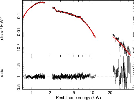
Combined broad-band Suzaku XIS-FI and PIN spectrum and ratios against the best-fitting model (red) of 4C+74.26 (number 1c) in the E = 0.6–70 keV energy band.
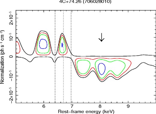
Energy–intensity contour plot in the interval E = 5–10 keV calculated using the broad-band spectrum of 4C+74.26 (number 1c), see text for more details. The arrows points the absorption line. The vertical lines refer to the energies of the neutral Fe Kα, Fe xxv and Fe xxvi lines at E = 6.4, 6.7 and 6.97 keV, respectively.
However, it is important to check the alternative interpretation of these emission residuals as due to reflection from the accretion disc and the check the effect on the modelling of the broad absorption. Initially, we model these emission residuals with a broad Gaussian emission line. The line parameters are |$E = 6.21^{+0.12}_{-0.25}$| keV, |$\sigma =438^{+81}_{-0.18}$| eV, |$I = (2.1^{+0.9}_{-0.3})$| photon s−1 cm−2 and EW = |$52^{+17}_{-13}$| eV. As we can see from panel 3 of Fig. A5 the inclusion of this broad line is able to model the residuals in emission at E ≃ 6–7 keV, but it still leaves absorption at higher energies. In fact, the best-fitting statistics in this case of χ2/ν = 2153.7/2117 is worse than the one derived including only the broad absorption line of χ2/ν = 2132.2/2117.
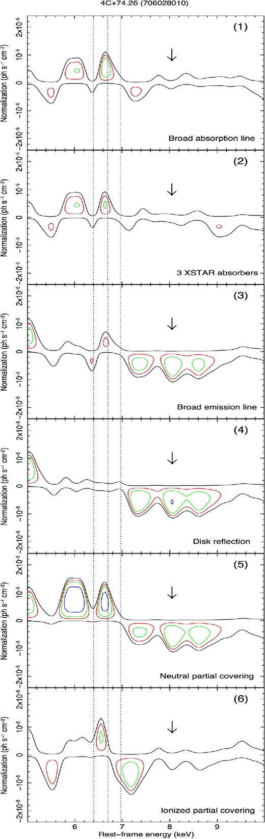
Energy–intensity contour plots of the spectrum of 4C+74.26 (number 1c) in the interval E = 5–10 keV. The different panels indicate the contours calculated using the broad-band model including a broad Gaussian absorption line (1), three xstar absorbers (2), a broad Gaussian emission line (3), disc reflection (4), a neutral (5) or ionized (6) partial covering absorber, respectively. The arrows points the absorption line. The vertical lines refer to the energies of the neutral Fe Kα, Fe xxv and Fe xxvi lines at E = 6.4, 6.7 and 6.97 keV, respectively.
The energy of the emission line indicates a possible identification with redshifted neutral Fe Kα emission originating from reflection off the accretion disc surrounding the central black hole. Therefore, we test a more physical model replacing the Gaussian emission line with a relativistically blurred (kdblur in xspec) pexmon component. We assume a maximally spinning black hole (a = 1), a standard emissivity index β = 3, an outer disc radius of rout = 400rg, an inclination angle of 30° and solar abundances. Given the limited quality of the data set, equivalent results are obtained using more complex models (Dauser et al. 2010, 2013; García et al. 2014). We estimate the inner radius of the reflecting surface of the disc of |$r_\rm{in} = 33^{+12}_{-8}r_{\rm g}$| and a moderate reflection fraction of R = 0.43 ± 0.06. This is consistent with the picture of a truncated disc in BLRGs, as previously reported for this (Larsson et al. 2008) and other sources (Ballantyne et al. 2004; Kataoka et al. 2007; Sambruna et al. 2009, 2011; Tombesi et al. 2011a, 2013b; Lohfink et al. 2013; Tazaki et al. 2013). Because of the contribution from disc reflection in both intensity of the Fe Kα and high-energy hump, the reflection fraction from distant material is slightly lower than the value reported in Table A2 of R = 0.18 ± 0.05. We obtain a good fit with χ2/ν = 2119.5/2118.
Best-fitting broad-band model of 4C+74.26 (number 1c).
| Warm absorber 1 | |
| NH (1022 cm−2) | |$0.30^{+0.06}_{-0.09}$| |
| log ξ (erg s−1 cm) | |$2.71^{+0.04}_{-0.05}$| |
| z | 0.104 |
| Warm absorber 2 | |
| NH (1022 cm−2) | 0.07 ± 0.01 |
| log ξ (erg s−1 cm) | <0.17a |
| z | 0.104 |
| Neutral reflection (pexmon) | |
| Γ | 1.76 ± 0.01 |
| R | 0.36 ± 0.03 |
| EC (keV) | 300 |
| AFe (solar) | 1 |
| i (°) | 30 |
| Absorption line | |
| E (keV) | 8.32 ± 0.18 |
| σ (eV) | |$900^{+200}_{-160}$| |
| I (10−5 photon s−1 cm−2) | |$-4.0^{+0.8}_{-0.9}$| |
| EW (eV) | −174 ± 37 |
| Absorption line statistics | |
| Δχ2/Δν | 38.7/3 |
| F-test (per cent) | ≫99.99 |
| MC (per cent) | >99.9 |
| Broad-band model statistics | |
| χ2/ν | 2132.3/2117 |
Note:a90 per cent upper limit.
From the contour plots in panel 4 of Fig. A5 we note that broad residuals in absorption at E > 7 keV are still present. In fact, the inclusion of a broad absorption line is still required at Δχ2/Δν = 32.2/2 with parameters consistent at the 1σ level with those listed in Table A2. We also checked that the inclusion of the three xstar absorption components is still required at a statistical level of Δχ2/Δν = 34/5 (corresponding to ≃4.5σ) and the parameters are consistent at the 90 per cent level with those discussed in Section A1.2. The best-fitting statistics in this case is χ2/ν = 2085.5/2113. Therefore, even including the possible presence of disc reflection, we find that the presence of the highly ionized absorber is still required with high significance.
Evidence for hard excesses at E > 10 keV possibly due to Compton-thick partial covering absorbers has been recently reported in a number of type 1 AGN (Tatum et al. 2013). From the ratios in Fig. A3 we do not see a significant hard excess at E > 10 keV in the Suzaku PIN data of this source, limiting the possible presence of such Compton-thick clouds along the line of sight of this source to have very low covering fractions. In fact, in Section A1.2 we already discussed the fact that the broad absorption at E > 7 keV cannot be adequately modelled with a fully covering neutral or ionized absorber at the source rest frame. However, it is important to check at what level the data can be explained by a partial covering absorber.
At first we include a neutral partial covering absorber modelled with zpcfabs in xspec. The resultant parameters are a column density is |$N_\rm{H} = (1.92^{+0.80}_{-0.43})\times 10^{24}$| cm−2 and a low covering fraction of Cf = 0.20 ± 0.04. The fit improvement of Δχ2/Δν = 24.7/2 is lower than in the case of the broad Gaussian absorption. Moreover, as we can see from the contours in panel 5 of Fig. A5, there are still absorption residuals at E > 7 keV. In fact, the inclusion of a broad absorption line with parameters consistent at the 1σ level with those reported in Table A2 is still required and provides a high fit improvement of Δχ2/Δν = 39.3/2.
Finally, we checked the possible modelling with an ionized partial covering absorber using zxipcf in xspec (Reeves et al. 2008). We obtain a high column density of |$N_\rm{H} = (1.34^{+0.07}_{-0.11})\times 10^{24}$| cm−2, a relatively high ionization parameter of log |$\xi = 2.69^{+0.06}_{-0.17}$| erg s−1 cm and a low covering fraction of Cf = 0.33 ± 0.03. As we can see from the panel 6 in Fig. A5, this model provides a relatively good representation of the data, leaving some emission/absorption residuals in the Fe K band. The best-fitting statistics is χ2/ν = 2102.9/2117. The goodness of fit parameter of the model including the disc reflection and broad Gaussian absorption or three xstar components is still slightly better. However, these are not nested models.
In order to get a more statistically reliable comparison, we start from the model including the disc reflection and include the ionized partial covering component. We obtain a fit improvement of Δχ2/Δν = 26.9/3. Instead, considering the alternative inclusion of a broad absorption line, we obtain a slightly higher fit improvement of Δχ2/Δν = 33.6/3. The statistical difference between the two is not very high.
Therefore, the Suzaku spectrum of the observation number 1c of 4C+74.26 shows complexities in the Fe K band both in emission and absorption which could be modelled as disc reflection and a fast ionized outflow or a single rest-frame partial covering ionized absorber. Given that we cannot strongly distinguish between these two models, we conservatively do not include the possible Fe K outflows detected in this observation in Table 1.
A2 3C 120
We analysed the combined Suzaku XIS-FI and PIN broad-band spectrum 3C 120 (observation number 9f) in the E = 0.6–70 keV energy band (excluding the interval E = 1.5–2 keV). The best-fitting model comprises a Galactic absorbed power-law continuum with Γ = 1.78 ± 0.01. There is no requirement for neutral absorption intrinsic to the source.
The neutral Fe Kα emission line is self-consistently modelled with a pexmon neutral reflection component with an inclination of i = 30°, high-energy cut-off of EC = 300 keV and standard solar abundances. We derive a relatively low reflection fraction of R = 0.39 ± 0.02, consistent with previous estimates (Ballantyne et al. 2004; Kataoka et al. 2007; Gofford et al. 2013; Lohfink et al. 2013). The width of the emission line is resolved and therefore we applied a multiplicative Gaussian smoothing of σ = 110 ± 10 eV.
We find an additional narrow emission line at the rest-frame energy of E = 6.85 ± 0.05 keV, possibly due to Fe xxv–xxvi. There is also a broad excess of emission in the soft X-rays which can be adequately parametrized with a blackbody component with kT = 0.38 ± 0.03 keV.
The fit improvement after the inclusion of a Gaussian absorption line at the rest-frame energy of E = 8.23 ± 0.04 keV is Δχ2/Δν = 12.5/2, corresponding to an F-test probability of 99.6 per cent. Given that the energy of the line is not directly consistent with that expected from ionized iron at rest, we also performed Monte Carlo simulations in order to better estimate its detection level as described in Section 4. The resultant Monte Carlo probability is 96.5 per cent. The final model provides a very good representation of the data, as shown in Fig. A6. The contour plot in the E = 5–10 keV energy band with respect to the baseline model without the inclusion of the absorption line is shown in Fig. A7. The best-fitting parameters are reported in Table A3.
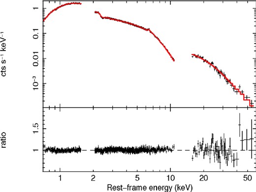
Combined broad-band Suzaku XIS-FI and PIN spectrum and ratios against the best-fitting model (red) of 3C 120 (number 9f) in the E = 0.6–70 keV energy band.
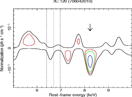
Energy–intensity contour plot in the interval E = 5–10 keV calculated using the broad-band spectrum of 3C 120 (number 9f), see text for more details. The arrows points the absorption line. The vertical lines refer to the energies of the neutral Fe Kα, Fe xxv and Fe xxvi lines at E = 6.4, 6.7 and 6.97 keV, respectively.
Best-fitting broad-band model of 3C 120 (number 9f).
| Blackbody | |
| kT (keV) | 0.38 ± 0.03 |
| N (10−5) | 1.3 ± 0.3 |
| Neutral reflection (pexmon) | |
| Γ | 1.78 ± 0.01 |
| R | 0.39 ± 0.02 |
| EC (keV) | 300 |
| AFe (solar) | 1 |
| i (°) | 30 |
| σ (eV) | 110 ± 10 |
| Emission line | |
| E (keV) | 6.85 ± 0.04 |
| σ (eV) | 10 |
| I (10−5 photon s−1 cm−2) | −0.60 ± 0.15 |
| EW (eV) | 12 ± 3 |
| Absorption line | |
| E (keV) | 8.23 ± 0.06 |
| σ (eV) | |$110^{+70}_{-62}$| |
| I (10−5 photon s−1 cm−2) | −0.70 ± 0.19 |
| EW (eV) | −20 ± 5 |
| Absorption line statistics | |
| Δχ2/Δν | 12.5/2 |
| F-test (per cent) | 99.6 |
| MC (per cent) | 96.5 |
| Broad-band model statistics | |
| χ2/ν | 2601.2/2510 |
If identified with Fe xxv Heα or Fe xxvi Lyα the absorption line would indicate a significant blueshifted velocity of ≃0.15–0.18c. We checked that the possible alternative modelling with a photoelectric edge provides a much worse fit (Δχ2/Δν = 3.8/2). The width of the absorption line can be loosely constrained at |$\sigma _E = 110^{+70}_{-62}$| eV, which corresponds to a velocity width of |$\sigma _v = 4000^{+2,600}_{-2,300}$| km s−1.
We performed a more physically self-consistent fit of this absorption line using the xstar table and the method described in Section 4. The velocity width of the line is consistent with the values of 3000 and 5000 km s−1 within the errors. Therefore, we used both xstar tables with these turbulent velocities. We find two equivalent fits at the 90 per cent and calculate the average. The best-fitting column density is NH > 2 × 1022 cm−2, the ionization parameter is log ξ = 4.91 ± 1.03 erg s−1 cm and the outflow velocity is vout = 0.161 ± 0.006c. The absorption is dominated by Fe xxv–xxvi ions and the velocity is consistent with a UFO. This modelling provides a good representation of the data, with a fit improvement with respect to the baseline model of Δχ2/Δν = 15.3/3, which corresponds to a confidence level of 99.5 per cent. The best-fitting xstar parameters are reported in the main text in Table 1.
We checked that the data do not significantly require the inclusion of a rest-frame neutral or ionized partial covering component using zpcfabs or zxipcf in xspec (Reeves et al. 2008). Therefore, these possible model complexities do not affect the results on the Fe K absorption lines for this observation.
The inclusion of a disc reflection component modelled with pexmon and relativistically blurred with kdblur in xspec provides only a marginal improvement to the fit of Δχ2/Δν = 8.6/2, corresponding to a confidence level of 98 per cent. We assume a maximally spinning black hole (a = 1), a standard emissivity index β = 3, an outer disc radius of rout = 400rg, an inclination angle of 30° and solar abundances. The inner radius of the disc reflecting surface is suggested to be relatively far away from the black hole at rin > 25rg and subsequently the reflection fraction is low R ≃ 0.2. This is consistent with previous evidences of a truncated disc in this source (e.g. Ballantyne et al. 2004; Kataoka et al. 2007), possibly linked with the disc–jet coupling (Lohfink et al. 2013).
Even including the possible weak disc reflection component, we find that the parameters of the Fe K absorber are consistent within the 1σ uncertainties. Therefore, this possible additional model component does not affect the results on the Fe K absorption lines for this observation.
A3 PKS 1549−79
We analysed the XMM–Newton EPIC-pn spectrum of PKS 1549−79 (observation number 12a) considering the observed energy range between E = 0.5 and 10.5 keV. No emission lines are detected in the Fe K band. The upper limits of the intensity and equivalent width of the 6.4 keV emission line are I < 2.2 × 10⁻⁶ photon s−1 cm−2 and EW < 18 eV. Therefore, a neutral reflection component was not included in the spectrum. The best-fitting model comprises a Galactic absorbed power-law continuum with Γ = 1.61 ± 0.03, intrinsic neutral absorption with column density NH = (5.2 ± 0.1) × 1022 cm−2 and a scattered continuum with a fraction of ≃2 per cent with respect to the direct one to model the soft excess.
As already reported in the E = 3.5–10.5 keV analysis, we find the presence of two absorption lines at the rest-frame energies of E = 9.15 ± 0.04 and 11.0 ± 0.04 keV, respectively. The F-test significance level is 99.9 per cent for each of them. This is slightly reduced to 99.1 and 98.8 per cent when compared to 1000 Monte Carlo simulations, respectively. The final model including these lines provides a very good representation of the data, as shown in Fig. A8. Given the relatively high redshift of PKS 1549−79 (z = 0.1522) and the high energies of the lines, in Fig. A9 we show the contour plot with respect to this model without the inclusion of absorption lines in the wider interval E = 5–12 keV. The best-fitting parameters are reported in Table A4.
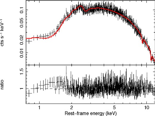
Broad-band XMM–Newton EPIC-pn spectrum and ratios against the best-fitting model (red) of PKS 1549−79 (number 12a) in the E = 0.7–12 keV energy band.
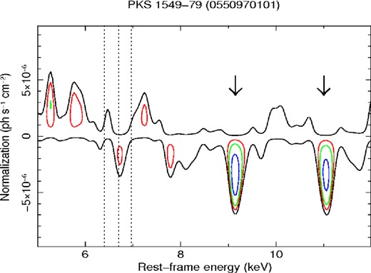
Energy–intensity contour plot in the interval E = 5–12 keV calculated using the broad-band spectrum of PKS 1549−79 (number 12a), see text for more details. The arrows points the absorption lines. The vertical lines refer to the energies of the neutral Fe Kα, Fe xxv and Fe xxvi lines at E = 6.4, 6.7 and 6.97 keV, respectively.
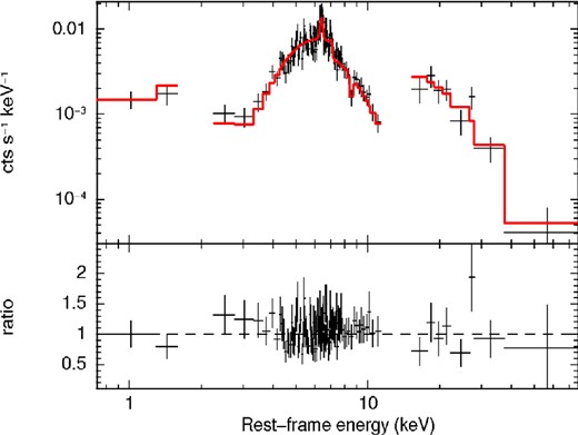
Combined broad-band Suzaku XIS-FI and PIN spectrum and ratios against the best-fitting model (red) of 3C 105 (number 16) in the E = 0.6–70 keV energy band.
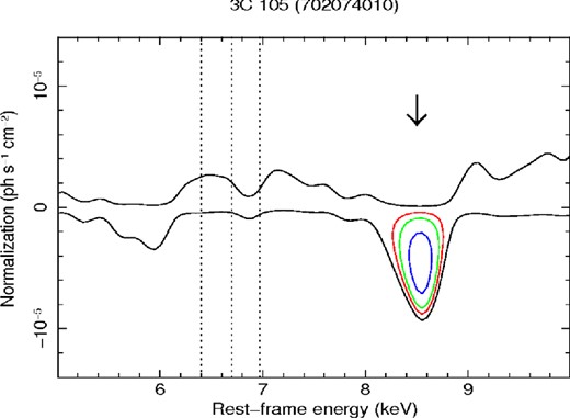
Energy–intensity contour plot in the interval E = 5–10 keV calculated using the broad-band spectrum of 3C 105 (number 16), see text for more details. The arrows points the absorption line. The vertical lines refer to the energies of the neutral Fe Kα, Fe xxv and Fe xxvi lines at E = 6.4, 6.7 and 6.97 keV, respectively.
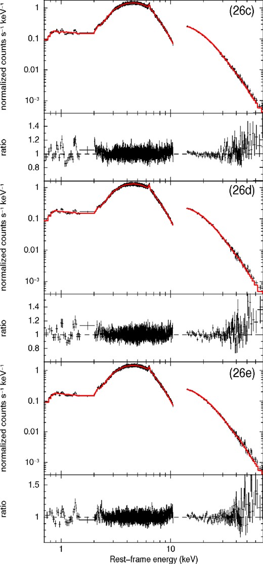
Combined broad-band Suzaku XIS-FI and PIN spectrum and ratios against the best-fitting model (red) of Centaurus A (numbers 26c, 26d, 26e) in the E = 0.6–70 keV energy band.
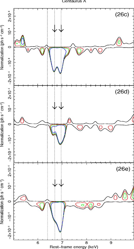
Energy–intensity contour plot in the interval E = 5–10 keV calculated using the broad-band spectrum of Centaurus A (numbers 26c, 26d and 26e), see text for more details. The arrows points the absorption lines. The vertical lines refer to the energies of the neutral Fe Kα, Fe xxv and Fe xxvi lines at E = 6.4, 6.7 and 6.97 keV, respectively.
Best-fitting broad-band model of PKS 1549−79 (number 12a).
| Neutral absorption | |
| NH (1022 cm−2) | 5.2 ± 0.1 |
| Power-law continuum | |
| ΓPow | 1.61 ± 0.03 |
| Scattered continuum | |
| ΓScatt | ΓPow |
| f (per cent) | ≃ 2 |
| Absorption line 1 | |
| E (keV) | 9.15 ± 0.04 |
| σ (eV) | 10 |
| I (10−5 photon s−1 cm−2) | −0.4 ± 0.1 |
| EW (eV) | −59 ± 15 |
| Absorption line 1 statistics | |
| Δχ2/Δν | 13.9/2 |
| F-test (per cent) | 99.9 |
| MC (per cent) | 99.1 |
| Absorption line 2 | |
| E (keV) | 11.0 ± 0.04 |
| σ (eV) | 10 |
| I (10−5 photon s−1 cm−2) | −0.4 ± 0.1 |
| EW (eV) | |$-80^{+21}_{-25}$| |
| Absorption line 2 statistics | |
| Δχ2/Δν | 13.3/2 |
| F-test (per cent) | 99.9 |
| MC (per cent) | 98.8 |
| Broad-band model statistics | |
| χ2/ν | 847.8/930 |
Best-fitting broad-band model of 3C 105 (number 16).
| Neutral absorption | |
| NH (1022 cm−2) | 41.3 ± 2.7 |
| Neutral reflection (pexmon) | |
| ΓPow | 1.80 ± 0.10 |
| R | |$1.26^{+0.34}_{-0.30}$| |
| EC (keV) | 300 |
| AFe (solar) | 1 |
| i (°) | 60 |
| Scattered continuum | |
| ΓScatt | ΓPow |
| f (per cent) | ≃1 |
| Absorption line | |
| E (keV) | 8.53 ± 0.05 |
| σ (eV) | 100 |
| I (10−5 photon s−1 cm−2) | −0.85 ± 0.24 |
| EW (eV) | −153 ± 41 |
| Absorption line statistics | |
| Δχ2/Δν | 11.6/2 |
| F-test (per cent) | 99.7 |
| MC (per cent) | 99.2 |
| Broad-band model statistics | |
| χ2/ν | 224.7/254 |
Best-fitting broad-band model of Centaurus A (number 26c, 26d and 26e).
| 26c | 26d | 26e | |
|---|---|---|---|
| Neutral absorption | |||
| NH (1022 cm−2) | 10.66 ± 0.04 | 10.80 ± 0.05 | 10.61 ± 0.04 |
| Neutral reflection (pexmon) | |||
| ΓPow | 1.850 ± 0.075 | 1.849 ± 0.009 | 1.831 ± 0.008 |
| R | 0.92 ± 0.04 | 1.04 ± 0.005 | 0.99 ± 0.04 |
| EC (keV) | 300 | 300 | 300 |
| AFe (solar) | 0.36 ± 0.02 | 0.41 ± 0.02 | 0.34 ± 0.02 |
| i (°) | 60 | 60 | 60 |
| Scattered continuum | |||
| ΓScatt | ΓPow | ΓPow | ΓPow |
| f (per cent) | ≃1 | ≃1 | ≃1 |
| Hot plasma (apec) | |||
| kT (keV) | 0.65 ± 0.02 | 0.65 ± 0.02 | 0.73 ± 0.02 |
| N (10−4) | 2.90 ± 0.15 | 2.90 ± 0.16 | 2.77 ± 0.14 |
| Absorption line 1 | |||
| E (keV) | 6.66 ± 0.02 | 6.64 ± 0.03 | 6.67 ± 0.02 |
| σ (eV) | 10 | 10 | 10 |
| I (10−5 photon s−1 cm−2) | −7.7 ± 0.9 | −3.4 ± 1.0 | −5.6 ± 1.0 |
| EW (eV) | −13 ± 2 | −7 ± 2 | −9 ± 2 |
| Absorption line 1 statistics | |||
| Δχ2/Δν | 63.7/2 | 11.3/2 | 30.0/2 |
| F-test (per cent) | ≫99.99 | 99.5 | >99.99 |
| Absorption line 2 | |||
| E (keV) | 6.95 ± 0.02 | 6.95 ± 0.02 | 6.93 ± 0.02 |
| σ (eV) | 10 | 10 | 10 |
| I (10−5 photon s−1 cm−2) | −8.4 ± 0.9 | −6.6 ± 1.0 | −9.6 ± 1.0 |
| EW (eV) | −16 ± 2 | −14 ± 2 | −18 ± 2 |
| Absorption line 2 statistics | |||
| Δχ2/Δν | 64.0/2 | 37.6/2 | 82.3/2 |
| F-test (per cent) | ≫99.99 | >99.99 | ≫99.99 |
| Broad-band model statistics | |||
| χ2/ν | 2830.7/2680 | 2858.0/2659 | 2848.8/2696 |
We checked that these narrow features cannot be modelled with two photoelectric edges. If identified with Fe xxv Heα or Fe xxvi Lyα these two absorption lines would indicate a high blueshifted velocity of ≃0.25c and ≃0.4c, respectively. Given the presence of two absorption lines, we checked their possible mutual identification as Fe xxv Heα (E = 6.7 keV) and Fe xxvi Lyα (E = 6.97 keV) or Fe xxv Heα and Heβ (E = 7.88 keV) or Fe xxvi Lyα and Lyβ (E = 8.25 keV) with a common blueshift. We included two absorption lines in the model with energies fixed to those expected for these transitions and let their common energy shift to vary. However, we find that the fit with two separated Gaussian absorption lines still provides a much better representation of the data, with a fit improvement higher than Δχ2/Δν = 10.5/1 with respect to the case with two lines with fixed energies and common shift.
We performed a more physically self-consistent fit of this absorption line using the xstar table and the method described in Section 4. Given that we can place only an upper limit of σv < 6000 km s−1 on the velocity width of these lines, we test three xstar tables with turbulent velocities of 1000, 3000 and 5000 km s−1, respectively. The fits using these three different turbulent velocities are equivalent at the 90 per cent level. Therefore, we took into account this degeneracy considering the average of their best-fitting parameters. We started with the inclusion of one xstar component to model the first line at E = 9.15 keV. This provides a fit improvement of Δχ2/Δν = 16.1/3 with respect to the baseline model, corresponding to a probability of 99.9 per cent. The best-fitting values of the column density, ionization parameter and outflow velocity are NH > 1 × 1023 cm−2, log ξ = 4.91 ± 0.53 erg s−1 cm and vout = 0.278 ± 0.006c, respectively.
However, including another xstar table provides a better representation of both absorption lines. Similarly to the case of observation number 1c of 4C+74.26 discussed in Section 4.1.2, the inclusion of another table with tied ionization parameter and column density provides a fit improvement higher than Δχ2/Δν = 8.9/1 with respect to the single xstar model, corresponding to a probability of 99.9 per cent. The new best-fitting ionization and column density are log ξ = 4.91 ± 0.49 erg s−1 cm and NH > 1.4 × 1023 cm−2, respectively. The two outflow velocities are vout = 0.276 ± 0.006c and 0.427 ± 0.005c, respectively. This provides a good modelling of both absorption lines. The fit improvement including both xstar tables with respect to the baseline model is high, Δχ2/Δν = 25/4, corresponding to a confidence level of 99.99 per cent (≥4σ). The best-fitting xstar parameters are reported in the main text in Table 1.
Therefore, the best fit of the two absorption lines at E ≃ 9.15 and ≃11 keV is provided by a highly ionized absorber with a somewhat complex velocity structure, which we modelled with two xstar components with high outflow velocities of 0.276c and 0.427c. These mildly relativistic velocities indicate the presence of a complex UFO in this source.
PKS 1549−79 was also observed with Suzaku (observation number 12b) about 1 month after XMM–Newton. The presence of the two blueshifted absorption lines indicative of UFOs cannot be excluded in the Suzaku observation at the 90 per cent level. In particular, an absorption line consistent with the one detected in the XMM–Newton spectrum at with E = 11.1 ± 0.1 keV and EW = −110 ± 51 eV is also independently detected in Suzaku, although at a lower significance of ∼92 per cent which falls below our detection threshold. This feature can be seen in the contour plots in Fig. C1 in Appendix C.
The inclusion of a possible rest-frame neutral partial covering component using zpcfabs in xspec with column density |$N_{\rm H} = (3.8^{+0.5}_{-0.4})\times 10^{22}$| cm−2 and |$C_{\rm f} = 0.84^{+0.13}_{-0.20}$| does not affect the results on the Fe K absorption lines. Moreover, as we can see from the lack of emission residuals in the contour plot in Fig. A9, the data do not require any broad emission line indicative of disc reflection.
A4 3C 105
We analysed the combined Suzaku XIS-FI and PIN broad-band spectrum 3C 105 (observation number 16) in the E = 0.6–70 keV energy band (excluding the interval E = 1.5–2 keV). The best-fitting model comprises a power-law continuum with Γ = 1.80 ± 0.10 absorbed by high column of neutral material with NH = (4.13 ± 0.27) × 1023 cm−2. A scattered continuum with a fraction of ≃1 per cent with respect to the direct one is present in the soft X-rays. The neutral Fe Kα emission line is self-consistently modelled with a pexmon neutral reflection component with an inclination of i = 60°, high-energy cut-off of EC = 300 keV and standard solar abundances. We derive a reflection fraction of |$R = 1.26^{+0.34}_{-0.30}$|.
The fit improvement after the inclusion of a Gaussian absorption line at the rest-frame energy of E = 8.53 ± 0.05 keV is Δχ2/Δν = 11.6/2, corresponding to an F-test probability of 99.7 per cent. Given that the energy of the line is not directly consistent with that expected from ionized iron at rest, we also performed Monte Carlo simulations in order to better estimate its detection level as described in Section 4. The resultant Monte Carlo probability is 99.2 per cent, higher than the selection threshold of 95 per cent. The final model provides a very good representation of the data, as shown in Fig. A10. The contour plot in the E = 5–10 keV energy band with respect to the baseline model without the inclusion of the absorption line is shown in Fig. A11. The best-fitting parameters are reported in Table A5.
If identified with Fe xxv Heα or Fe xxvi Lyα the absorption line would indicate a significant blueshifted velocity of ≃0.2c. We checked that the possible alternative modelling with a photoelectric edge provides a much worse fit (Δχ2/Δν = 1.5/2).
The width of the absorption line in the Suzaku spectrum of 3C 105 is not well constrained and we can place an upper limit of σv < 6000 km s−1. Therefore, we performed fits using three xstar tables with turbulent velocities of 1000, 3000 and 5000 km s−1, respectively. We obtain equivalent fits at the 90 per cent level in the three cases. For each of them we also find a degeneracy in the identification of the line with Fe xxv or Fe xxvi. Therefore, we consider an average among these six solutions with column density NH > 2 × 1022 cm−2, ionization parameter log ξ = 3.81 ± 1.30 erg s−1 cm and outflow velocity of vout = 0.227 ± 0.033c. This highly ionized absorber has a velocity that is consistent with a UFO. The model provides a good representation of the data, with a fit improvement of Δχ2/Δ/ν = 10.5/3, corresponding to a confidence level of 99 per cent. The best-fitting xstar parameters are reported in the main text in Table 1.
We checked that the data do not significantly require the inclusion of a rest-frame neutral or ionized partial covering component using zpcfabs or zxipcf in xspec (Reeves et al. 2008). Moreover, as we can see from the lack of emission residuals in the contour plot in Fig. A11, the data do not require any broad emission line indicative of disc reflection. Therefore, these possible model complexities do not affect the results on the Fe K absorption lines for this observation.
A5 Centaurus A
We analyse the combined Suzaku XIS-FI and PIN broad-band spectrum of Centaurus A (observation number 26c) in the energy band E = 0.6–70 keV (excluding the interval E = 1.5–2 keV). As already reported for the E = 3.5–10.5 keV analysis in Table A2 in Appendix A, the spectrum is well described by a neutral absorbed power-law continuum with NH = (10.66 ± 0.04) × 1022 cm−2 and Γ = 1.850 ± 0.075.
The neutral Fe Kα emission line is self-consistently modelled with a pexmon neutral reflection component with an inclination fixed to i = 60° and high-energy cut-off of EC = 300 keV (e.g. Dadina 2007). We obtain a reflection fraction of R = 0.92 ± 0.04 and an iron abundance lower than solar, of AFe = 0.36 ± 0.02. The soft X-ray part of the spectrum requires a scattered continuum component with a fraction of ≃1 per cent and a hot plasma emission modelled with apec in xspec with a temperature of kT = 0.65 ± 0.02 keV.
We find the presence of two narrow absorption lines at the rest-frame energies of E = 6.66 ± 0.02 and 6.95 ± 0.02 keV, respectively. Their significance level is very high, being ≫99.99 per cent for both of them. The energies of these features clearly favour an interpretation as resonance absorption lines from Fe xxv Heα at E = 6.7 keV and Fe xxvi Lyα at E = 6.97 keV, respectively. Given that the lines are consistent with the expected values, the standard F-test can be applied and there is no need to perform additional Monte Carlo simulations. The final model provides a very good representation of the data, as shown in Fig. A12. The contour plot in the E = 5–10 keV energy band with respect to the baseline model without the inclusion of the absorption lines is shown in Fig. A13. The best-fitting parameters are reported in Table A6.
The best-fitting model derived for observation number 26c is also applicable to the subsequent Suzaku observations 23d and 23e. These observations were performed in a period of about 3 weeks. The fit parameters are equivalent. In particular, the two narrow absorption lines are still observed at the same energies with a statistical confidence level always higher than 99.5 per cent. There is only a slight change in the equivalent width. The final models for observations 26d and 26e provide a very good representation of the data, as shown in Fig. A12. The contour plots in the E = 5–10 keV band are shown in Fig. A13 and their best-fitting parameters are reported in Table A6.
The energies of the detected absorption lines are directly consistent with Fe xxv Heα and Fe xxvi Lyα. The absorption lines are narrow and we can place a 90 per cent upper limit of σv < 5000 km s−1. We performed a more physically self-consistent fit using the xstar table and the method described in Section 4. We test xstar tables with turbulent velocities of 1000, 3000 and 5000 km s−1, respectively. For each observation we average the values of the parameters for xstar solutions with different turbulent velocities but equivalent best fits at the 90 per cent level. Given that the energy of the lines is consistent with the expected values, we fixed the shift of the absorption components to zero. The best-fitting values of the column density and ionization parameter for observation number 26c are NH = (4.2 ± 0.4) × 1022 cm−2 and log ξ = 4.33 ± 0.03 erg s−1 cm, respectively. The fit improvement is Δχ2/Δν = 126.5/2, corresponding to a very high confidence level of ≫99.99 per cent.
The best-fitting parameters for the observation number 26d are |$N_\rm{H}= (4.1^{+0.9}_{-1.0})\times 10^{22}$| cm−2 and log |$\xi = 4.37^{+0.03}_{-0.05}$| erg s−1 cm. The fit improvement is Δχ2/Δν = 54.7/2, corresponding to a high confidence level of ≫99.99 per cent. Finally, the best-fitting values of the column density and ionization parameter for observation number 26e are NH = (4.0 ± 1.1) × 1022 cm−2 and log ξ = 4.31 ± 0.10 erg s−1 cm, respectively. The fit improvement is Δχ2/Δν = 105.3/2, corresponding to a very high confidence level of ≫99.99 per cent. Leaving the outflow velocity free, we derive upper limits of vout < 1100, <1500 and <800 km s−1 for the observation number 26c, 26d and 26e, respectively. The best-fitting xstar parameters of these three observations are consistent with each other and they are reported in the main text in Table 1.
We note that this spectral analysis of this data set was already reported by Fukazawa et al. (2011). The authors did not perform a detailed search for Fe K absorption lines, but indeed suggested that the spectral variability of this source may be influenced by a complex nuclear absorber.
APPENDIX B: LONG TABLES
If identified as Fe xxv Heα or Fe xxvi Lyα the absorption line would indicate a significant blueshifted velocity of ≃0.04–0.08c (≃12 000–24 000 km s−1). We checked that this narrow feature cannot be modelled with a photoelectric edge. The upper limit of the width of the absorption line is σv < 12 000 km s−1.
We performed a more physically self-consistent fit of this absorption line using the xstar table and the method described in Section 4. Given that the velocity width of the line is not well constrained, we performed fits using three xstar tables with turbulent velocities of 1000, 3000 and 5000 km s−1, respectively. For each case, we find a single solution indicating a preferred identification of the absorption line as Fe xxvi Lyα. However, the best fits using the three different turbulent velocities are equivalent at the 90 per cent level. We took into account this degeneracy in turbulent velocity calculating the average of the best-fitting parameters. The best-fitting values of the column density, ionization parameter and outflow velocity are NH > 5 × 1022 cm−2, log ξ = 4.62 ± 0.25 erg s−1 cm and vout = 0.045 ± 0.008c, respectively. The outflow velocity of 13 500 ± 2400 km s−1 is consistent with a UFO. This modelling provides a good representation of the data, with a fit improvement with respect to the baseline model of Δχ2/Δν = 13.7/3, which corresponds to a confidence level of 99.6 per cent. The best-fitting xstar parameters are reported in the main text in Table 1.
We checked that the data do not significantly require the inclusion of a rest-frame neutral or ionized partial covering component using zpcfabs or zxipcf in xspec (Reeves et al. 2008). Moreover, as we can see from the lack of emission residuals in the contour plot in Fig. A2, the data do not require any broad emission line indicative of disc reflection. Therefore, these possible model complexities do not affect the results on the Fe K absorption lines for this observation.
A1.2 Observation 1c
We analysed the combined Suzaku XIS-FI and PIN broad-band spectrum 4C+74.26 (observation number 1c) in the E = 0.6–70 keV energy band (excluding the E = 1.5–2 keV interval). The best-fitting model comprises a Galactic absorbed power-law continuum with Γ = 1.76 ± 0.01. From the E = 3.5–10.5 keV analysis reported in Table B2 in Appendix B we see that the energy of the Fe Kα emission line in this observation of E = 6.38 ± 0.02 keV is consistent with neutral material. Therefore, an ionized reflection component is not required in this observation and we include a pexmon component with an inclination of i = 30°, high-energy cut-off of EC = 300 keV and standard solar abundances. We obtain a reflection fraction of R = 0.36 ± 0.03.
List of radio-loud AGN with relative XMM–Newton and Suzaku observations.
| Num | Source | z | Sy | FR | Obs | OBSID | Date | Counts | Exp | Flux | Lum | Abs |
|---|---|---|---|---|---|---|---|---|---|---|---|---|
| (1) | (2) | (3) | (4) | (5) | (6) | (7) | (8) | (9) | (10) | (11) | (12) | (13) |
| 1a | 4C+74.26 | 0.1040 | 1 | II | X | 0200910201 | 2004-02-06 | 27 800/112 | 26.6 | 15.0 | 40.0 | |
| 1b | S | 702057010 | 2007-10-28 | 58 631/1751 | 91.6 | 19.0 | 51.0 | Yd | ||||
| 1c | S | 706028010 | 2011-11-23 | 67 814/706 | 101.4 | 16.0 | 44.0 | |||||
| 2a | PKS 0558−504 | 0.1372 | 1 | – | X | 0129360201 | 2000-10-10 | 3399/38 | 7.5 | 6.2 | 32.0 | |
| 2b | X | 0137550201 | 2001-06-26 | 1779/51 | 10.5 | 6.5 | 33.0 | |||||
| 2c | X | 0137550601 | 2001-10-19 | 3288/60 | 10.2 | 12.0 | 63.0 | |||||
| 2d | X | 0555170201 | 2008-09-07 | 30 651/1112 | 71.2 | 5.8 | 30.0 | |||||
| 2e | X | 0555170301 | 2008-09-09 | 31 709/913 | 78.7 | 5.5 | 28.0 | |||||
| 2f | X | 0555170401 | 2008-09-11 | 48 304/2223 | 86.4 | 7.6 | 39.0 | |||||
| 2g | S | 701011010 | 2007-01-17 | 5493/277 | 20.6 | 6.0 | 31.0 | |||||
| 2h | S | 701011020 | 2007-01-18 | 6927/274 | 18.9 | 8.1 | 42.0 | |||||
| 2i | S | 701011030 | 2007-01-19 | 5368/288 | 21.3 | 5.8 | 29.0 | |||||
| 2l | S | 701011040 | 2007-01-20 | 8137/286 | 19.8 | 9.4 | 48.0 | |||||
| 2m | S | 701011050 | 2007-01-21 | 7211/269 | 19.5 | 8.3 | 43.0 | |||||
| 3 | 3C 332 | 0.1510 | 1 | II | S | 704038010 | 2009-08-08 | 9362/870 | 59.9 | 3.8 | 22.0 | |
| 4a | 3C 382 | 0.0578 | 1 | II | X | 0506120101 | 2008-04-28 | 36 824/675 | 22.0 | 23.0 | 18.0 | |
| 4b | S | 702125010 | 2007-04-27 | 145 739/2370 | 130.6 | 27.0 | 21.0 | Na, d, e | ||||
| 5 | 3C 059 | 0.1097 | 1.8 | – | X | 0205390201 | 2004-07-30 | 17 939/255 | 47.1 | 5.5 | 16.0 | |
| 6a | 3C 390.3 | 0.0561 | 1.5 | II | X | 0203720201 | 2004-10-08 | 60 103/607 | 36.1 | 24.0 | 18.0 | |
| 6b | X | 0203720301 | 2004-10-17 | 32 896/265 | 22.5 | 21.0 | 15.0 | |||||
| 6c | S | 701060010 | 2006-12-14 | 81 187/1236 | 99.4 | 20.0 | 15.0 | Ya, d | ||||
| 7a | 3C 111 | 0.0485 | 1 | II | X | 0552180101 | 2009-02-15 | 116 320/1532 | 55.0 | 31.0 | 17.0 | Nb |
| 7b | S | 703034010 | 2008-08-22 | 55 621/2499 | 122.4 | 13.0 | 7.4 | Ya, b, d | ||||
| 7c | S | 705040010 | 2010-09-02 | 100 435/1117 | 80.6 | 30.0 | 17.0 | Nc, d | ||||
| 7d | S | 705040020 | 2010-09-09 | 126 335/1147 | 79.4 | 38.0 | 21.0 | Yc, d | ||||
| 7e | S | 705040030 | 2010-09-14 | 123 357/1246 | 80.4 | 36.0 | 20.0 | Nc, d | ||||
| 8 | 3C 206 | 0.0860 | 1.2 | II | S | 705007010 | 2010-05-08 | 17 729/1012 | 80.6 | 6.4 | 12.0 | |
| 9a | 3C 120 | 0.0330 | 1.5 | I | X | 0152840101 | 2003-08-26 | 166 430/1681 | 85.9 | 28.0 | 6.9 | |
| 9b | S | 700001010 | 2006-02-09 | 80 076/1885 | 41.9 | 28.0 | 7.0 | Na, d | ||||
| 9c* | S | 700001020 | 2006-02-16 | 69 754/1789 | 41.6 | 25.0 | 6.2 | Ya, d | ||||
| 9d* | S | 700001030 | 2006-02-23 | 69 241/1775 | 40.9 | 25.0 | 6.2 | Ya, d | ||||
| 9e* | S | 700001040 | 2006-03-02 | 66 260/1629 | 40.9 | 25.0 | 6.0 | Ya, d | ||||
| 9f | S | 706042010 | 2012-02-09 | 227 512/5834 | 183.0 | 30.0 | 7.5 | |||||
| 9g | S | 706042020 | 2012-02-14 | 144 163/3697 | 118.0 | 29.0 | 7.3 | |||||
| 10a | 4C+50.55 | 0.0200 | 1 | II | X | 0306320201 | 2005-11-06 | 50 289/101 | 21.6 | 36.0 | 3.3 | |
| 10b | S | 702027010 | 2007-04-16 | 142 711/2764 | 85.0 | 51.0 | 4.9 | |||||
| 11 | Pictor A | 0.0351 | 3b | II | X | 0206390101 | 2005-01-14 | 12 356/304 | 40.7 | 6.5 | 1.8 | |
| 12a | PKS 1549−79 | 0.1522 | 1i | II | X | 0550970101 | 2008-09-21 | 14 525/296 | 48.2 | 4.3 | 29.0 | |
| 12b | S | 703059010 | 2008-10-13 | 12 205/751 | 82.2 | 3.6 | 25.0 | |||||
| 13 | 3C 234 | 0.1850 | 1.9 | II | X | 0405340101 | 2006-04-24 | 1894/132 | 26.6 | 1.2 | 15.0 | |
| 14 | PKS 0707−35 | 0.1108 | – | II | S | 706008010 | 2011-04-02 | 11 373/474 | 81.2 | 3.9 | 13.0 | |
| 15 | PKS 2356−61 | 0.0963 | 2 | II | S | 801016010 | 2006-12-06 | 10 765/639 | 100.9 | 2.9 | 9.4 | |
| 16 | 3C 105 | 0.0890 | 2 | II | S | 702074010 | 2008-02-05 | 2126/414 | 37.4 | 2.1 | 8.0 | |
| 17 | PKS 0326−288 | 0.1088 | 2 | – | S | 704039010 | 2010-01-30 | 1692/332 | 58.0 | 0.9 | 6.5 | |
| 18a | 3C 445 | 0.0558 | 1.5 | II | X | 0090050601 | 2001-12-16 | 5676/63 | 15.4 | 5.9 | 5.8 | |
| 18b | S | 702056010 | 2007-05-25 | 30 259/1459 | 139.7 | 6.1 | 7.0 | Ya, d, f, g | ||||
| 19 | 3C 433 | 0.1016 | 2 | II | S | 705050010 | 2010-11-06 | 4686/326 | 62.6 | 2.2 | 6.3 | |
| 20a | 3C 452 | 0.0811 | 2 | II | X | 0552580201 | 2008-11-30 | 6770/304 | 54.2 | 2.2 | 5.5 | |
| 20b | S | 702073010 | 2007-06-16 | 3274/368 | 66.7 | 2.0 | 4.3 | |||||
| 21a | 3C 33 | 0.0597 | 2 | II | X | 0203280301 | 2004-01-21 | 870/20 | 6.3 | 2.5 | 3.9 | |
| 21b | S | 702059010 | 2007-12-26 | 9165/1191 | 127.4 | 2.6 | 4.0 | |||||
| 22a | NGC 612 | 0.0298 | 2 | II | X | 0312190201 | 2006-06-26 | 778/90 | 9.6 | 1.7 | 2.1 | |
| 22b | S | 703016010 | 2008-05-20 | 1502/280 | 48.5 | 1.5 | 1.4 | |||||
| 23 | 4C+29.30 | 0.0647 | 2 | II | X | 0504120101 | 2008-04-11 | 630/106 | 17.5 | 0.6 | 1.3 | |
| 24 | 3C 403 | 0.0590 | 2 | II | S | 704011010 | 2009-04-08 | 760/288 | 47.9 | 0.6 | 0.9 | |
| 25 | IC 5063 | 0.0114 | 1h | I | S | 704010010 | 2009-04-24 | 9236/569 | 45.2 | 7.3 | 0.4 | |
| 26a | Centaurus A | 0.0018 | 2 | I | X | 0093650201 | 2001-02-02 | 26 596/160 | 16.7 | 170.0 | 0.2 | |
| 26b | X | 0093650301 | 2002-02-06 | 13 687/83 | 7.9 | 180.0 | 0.2 | |||||
| 26c | S | 704018010 | 2009-07-20 | 584 087/9497 | 62.6 | 280.0 | 0.3 | |||||
| 26d | S | 704018020 | 2009-08-05 | 431 570/7464 | 51.3 | 250.0 | 0.2 | |||||
| 26e | S | 704018030 | 2009-08-14 | 527 093/8571 | 55.9 | 280.0 | 0.3 |
Notes: (1) Object number. Letters are used to enumerate multiple observations. (2) Object name. (3) Cosmological redshift. (4) Optical identification and reference, by referring Véron-Cetty & Véron (2010). Sy1i and Sy1h show the sources with broad Paschen lines in the infrared and with broad polarized Balmer lines, respectively. The source identified as S3b is Seyfert 3 of liner with broad Balmer lines. (5) Fanaroff–Riley (FR) type. (6) Observatory, X if XMM–Newton and S if Suzaku, respectively. (7) Observation ID. (8) Start date of the observation in yyyy-mm-dd. (9) Source/background counts in the E = 4–10 keV band. Data are relative to the EPIC-pn or XIS-FI if corresponding to XMM–Newton or Suzaku, respectively. (10) Net exposure in units of ks. (11) Observed flux in the E = 4–10 keV band in units of 10−12 erg s−1 cm. (12) Absorption corrected luminosity in the E = 4–10 keV band in units of 1043 erg s−1. (13) Y (or N) indicate if (or if not) a detailed Fe K absorption line search was already reported in the literature and if any line was (was not) detected.
a, b, c, d, e, f and g indicate that the observation was already analysed in detail by Tombesi et al. (2010a), Ballo et al. (2011), Tombesi et al. (2011a), Gofford et al. (2013), Sambruna et al. (2011), Braito et al. (2011) and Reeves et al. (2010), respectively.
*Indicates that the consecutive observations have been added together and were considered as a single one in the spectral analysis.
Baseline model parameters of the spectra in the E = 3.5–10.5 keV band. We consider only observations without Fe K absorption line searches reported in the literature.
| Num | Source | NH, Gal | Γ | NH | E | σ | I | EW | χ2/ν | Abs |
|---|---|---|---|---|---|---|---|---|---|---|
| (1) | (2) | (3) | (4) | (5) | (6) | (7) | (8) | (9) | (10) | (11) |
| 1a | 4C+74.26 | 12 | 1.67 ± 0.02 | 6.50 ± 0.04 | 100 | 1.8 ± 0.3 | 56 ± 10 | 849/830 | Y | |
| 1c | 1.79 ± 0.01 | 6.38 ± 0.02 | 100 | 2.6 ± 0.2 | |$74^{+6}_{-4}$| | 1304/1334 | Y | |||
| 2a | PKS 0558−504 | 4 | 2.12 ± 0.06 | 127/157 | N | |||||
| 2b | 2.02 ± 0.08 | 72/88 | N | |||||||
| 2c | 2.19 ± 0.06 | 142/156 | N | |||||||
| 2d | 2.04 ± 0.02 | 834/852 | N | |||||||
| 2e | 2.03 ± 0.02 | 800/859 | N | |||||||
| 2f | 2.03 ± 0.02 | 1082/1000 | N | |||||||
| 2g | 2.10 ± 0.05 | 258/255 | N | |||||||
| 2h | 2.21 ± 0.04 | 310/314 | N | |||||||
| 2i | 2.01 ± 0.05 | 273/252 | N | |||||||
| 2l | 2.09 ± 0.04 | 344/362 | N | |||||||
| 2m | 2.18 ± 0.04 | 308/325 | N | |||||||
| 3 | 3C 332 | 2 | 1.56 ± 0.04 | 6.42 ± 0.08 | 100 | 0.5 ± 0.1 | |$58^{+14}_{-16}$| | 416/413 | N | |
| 4a | 3C 382 | 7 | 1.76 ± 0.01 | 6.42 ± 0.01 | 87 ± 18 | 2.6 ± 0.3 | 52 ± 5 | 1631/1599 | N | |
| 5 | 3C 059 | 6 | 1.55 ± 0.03 | 580/642 | N | |||||
| 6a | 3C 390.3 | 4 | 1.62 ± 0.02 | |$6.49^{+0.09}_{-0.05}$| | |$186^{+149}_{-84}$| | |$2.2^{+1.0}_{-0.6}$| | 50 ± 9 | 1113/1084 | N | |
| 6b | 1.62 ± 0.02 | 6.44 ± 0.02 | 70 ± 33 | 2.3 ± 0.4 | 58 ± 9 | 1012/896 | N | |||
| 8 | 3C 206 | 6 | 1.75 ± 0.03 | 670/687 | N | |||||
| 9a | 3C 120 | 10 | 1.74 ± 0.01 | 6.42 ± 0.01 | 86 ± 14 | 3.1 ± 0.3 | 62 ± 5 | 1323/1314 | N | |
| 6.96 ± 0.02 | 10 | 0.9 ± 0.2 | 21 ± 4 | |||||||
| 9f | 1.76 ± 0.01 | 6.37 ± 0.01 | 92 ± 16 | 3.9 ± 0.3 | 71 ± 5 | 1780.0/1737 | Y | |||
| 6.85 ± 0.03 | |$125^{+35}_{-32}$| | 1.5 ± 0.3 | 31 ± 8 | |||||||
| 9g | 1.81 ± 0.01 | 6.37 ± 0.01 | 108 ± 19 | 3.8 ± 0.3 | |$72^{+5}_{-7}$| | 1573/1603 | N | |||
| 6.91 ± 0.03 | 10 | 1.0 ± 0.2 | 21 ± 4 | |||||||
| 10a | 4C+50.55 | 100 | 1.35 ± 0.02 | 6.40 ± 0.04 | 100 | 1.7 ± 0.5 | 27 ± 8 | 1134/1066 | N | |
| 10b | 1.71 ± 0.02 | 2 ± 1 | 6.37 ± 0.03 | 100 | 2.7 ± 0.4 | 28 ± 5 | 1687/1601 | N | ||
| 11 | Pictor A | 3 | 1.73 ± 0.03 | 6.44 ± 0.05 | 100 | 0.7 ± 0.2 | 61 ± 17 | 454/479 | N | |
| 12a | PKS 1549−79 | 10 | 1.78 ± 0.06 | 6 ± 1 | 511/540 | Y | ||||
| 12b | 1.93 ± 0.07 | 6 ± 1 | 466/493 | N | ||||||
| 13 | 3C 234 | 2 | 1.40 ± 0.23 | 25 ± 5 | 6.43 ± 0.04 | 94 ± 42 | 0.9 ± 0.2 | 216 ± 40 | 89/83 | N |
| 14 | PKS 0707−35 | 16 | 1.75 ± 0.08 | 5 ± 1 | 6.39 ± 0.02 | 10 | 0.6 ± 0.1 | |$66^{+14}_{-12}$| | 477/463 | N |
| 15 | PKS 2356−61 | 2 | 1.85 ± 0.08 | 17 ± 2 | 467/436 | N | ||||
| 16 | 3C 105 | 10.2 | 1.35 ± 0.23 | 35 ± 4 | 6.39 ± 0.03 | 100 | 1.7 ± 0.3 | |$214^{+94}_{-33}$| | 111/101 | Y |
| 17 | PKS 0326−288 | 1 | 1.83 ± 0.31 | 47 ± 7 | 6.40 ± 0.04 | |$138^{+66}_{-54}$| | 1.3 ± 0.3 | |$275^{+77}_{-57}$| | 127/81 | N |
| 18a | 3C 445 | 5 | 1.22 ± 0.12 | 15 ± 2 | 6.38 ± 0.03 | |$107^{+43}_{-37}$| | 2.1 ± 0.4 | |$145^{+31}_{-35}$| | 230/227 | N |
| 19 | 3C 433 | 12 | 1.69 ± 0.13 | 6 ± 2 | 6.46 ± 0.03 | 10 | 0.4 ± 0.1 | |$83^{+27}_{-22}$| | 195/214 | N |
| 20a | 3C 452 | 10 | 0.80 ± 0.20 | 21 ± 3 | 6.40 ± 0.01 | 71 ± 21 | 1.4 ± 0.2 | |$285^{+38}_{-35}$| | 124/145 | N |
| 20b | 0.87 ± 0.12 | 29 ± 3 | 6.42 ± 0.02 | 92 ± 23 | 1.6 ± 0.2 | |$245^{+52}_{-22}$| | 271/265 | N | ||
| 21a | 3C 33 | 4 | 1.25 ± 0.31 | 34 ± 6 | 6.40 ± 0.05 | |$95^{+59}_{-46}$| | 2.0 ± 0.6 | |$243^{+53}_{-59}$| | 35/32 | N |
| 21b | 1.44 ± 0.11 | 32 ± 2 | 6.38 ± 0.01 | 100 | 1.6 ± 0.1 | |$180^{+20}_{-10}$| | 420/385 | N | ||
| 22a | NGC 612 | 2 | 1.67 ± 0.36 | 98 ± 12 | 32/34 | N | ||||
| 22b | 1.38 ± 0.29 | 84 ± 8 | 6.40 ± 0.02 | 10 | 2.8 ± 0.5 | 246 ± 45 | 45/68 | N | ||
| 23 | 4C+29.30 | 4 | 1.34 ± 0.44 | 38 ± 9 | 6.41 ± 0.04 | |$118^{+45}_{-42}$| | 1.0 ± 0.2 | |$437^{+196}_{-107}$| | 24/26 | N |
| 24 | 3C 403 | 15 | 1.20 ± 0.50 | 31 ± 11 | 6.44 ± 0.02 | 85 ± 31 | 1.3 ± 0.2 | |$69^{+19}_{-10}$| | 48/40 | N |
| 25 | IC 5063 | 6 | 1.84 ± 0.10 | 25 ± 2 | 6.40 ± 0.01 | 84 ± 21 | 4.2 ± 0.5 | |$194^{+26}_{-20}$| | 347/362 | N |
| 26a | Centaurus A* | 8 | 1.91 ± 0.08 | 11.7 ± 0.8 | 6.41 ± 0.02 | 10 | 35.3 ± 3.7 | |$88^{+12}_{-8}$| | 672/740 | N |
| 26b | 1.83 ± 0.10 | 12.4 ± 1.1 | 6.40 ± 0.02 | 10 | 50.4 ± 5.7 | |$115^{+17}_{-9}$| | 426/409 | N | ||
| 26c | 1.82 ± 0.01 | 10.7 ± 0.2 | 6.388 ± 0.003 | 10 | 35.8 ± 1.1 | 58 ± 2 | 2042/1909 | Y | ||
| 26d | 1.83 ± 0.01 | 11.3 ± 0.2 | 6.393 ± 0.003 | 10 | 38.4 ± 1.1 | 69 ± 2 | 2004/1889 | Y | ||
| 26e | 1.80 ± 0.01 | 10.9 ± 0.2 | 6.391 ± 0.003 | 10 | 36.0 ± 1.1 | 58 ± 2 | 2009/1908 | Y |
Notes: (1) Object number. Letters are used to enumerate multiple observations. (2) Object name. (3) Galactic column density in units of 1020 cm−2. (4) Power-law photon index. (5) Neutral absorption column density in units of 1022 cm−2. (6)–(9) Emission line energy, width, intensity and equivalent width in units of keV, eV, 10−5 photon s−1 cm−2 and eV, respectively. (10) Best-fitting χ2 over degrees of freedom ν. (11) Presence (or not) of absorption lines at rest-frame energies E > 6 keV in the energy–intensity contour plots.
*Given the high flux and S/N of the observations of Centaurus A, we included neutral reflection pexrav component in xspec with reflection fraction R = 1, high-energy cut-off EC = 300 keV and inclination of i = 60°.
As already reported in the literature, the soft X-ray spectrum of 4C+74.26 shows intense O vii and O viii absorption edges indicative of ionized material along the line of sight (Ballantyne 2005; Gofford et al. 2013). As already discussed in the previous section, these features are well parametrized with the inclusion of two warm absorber components. Therefore, we use again two xstar tables with a typical Γ = 2 ionizing continuum and turbulent velocity of 100 km s−1. Given the relatively low energy resolution of the XIS spectrum in the soft X-rays, we cannot reliably constrain their possible velocity shifts, which were fixed to zero. The fit improvement after including these two ionized warm absorbers is very high, Δχ2/Δν = 251.2/4, indicating a confidence level of ≫99.99 per cent. It should be noted that a neutral absorption component is not formally required in this fit, but the value of the ionization parameter of the second warm absorber is much lower than in the previous observation.
As we can see in the contour plot in Fig. C1, there is evidence for a broad absorption trough at energies of E ≃ 7–10 keV. Including a Gaussian absorption line at the rest-frame energy of E ≃ 8 keV with free width we find a high fit improvement (Δχ2/Δν = 38.7/3), which corresponds to an F-test confidence level of 5.5σ. The line has a rest-frame energy of E = 8.32 ± 0.18 keV, a width of |$\sigma = 900^{+200}_{-160}$| eV, intensity |$I = (-4.0^{+0.8}_{-0.9})\times 10^{-5}$| photon s−1 cm−2 and EW=−174 ± 37 eV. Given that the energy of the line is not directly consistent with that expected from ionized iron at rest, we also performed Monte Carlo simulations in order to better estimate its detection level as described in Section 4. The resultant Monte Carlo probability is >99.9 per cent, which is much higher than the selection threshold of 95 per cent. The final model provides a very good representation of the data, as shown in Fig. A3. The contour plot in the E = 5–10 keV energy band with respect to the baseline model without the inclusion of the absorption line is shown in Fig. A4. The best-fitting parameters are listed in Table A2.
APPENDIX C: RATIOS AND CONTOUR PLOTS
![Ratio against the continuum (upper panel) and contour plots with respect to the best-fitting baseline model [lower panel; 68 per cent (red), 90 per cent (green), 99 per cent (blue) levels] for the radio-loud sources. The Fe K absorption lines are pointed by arrows. The vertical lines refer to the neutral Fe Kα, Fe xxv and Fe xxvi lines at E = 6.4, 6.7 and 6.97 keV, respectively.](https://oup.silverchair-cdn.com/oup/backfile/Content_public/Journal/mnras/443/3/10.1093/mnras/stu1297/2/m_stu1297figc1a.jpeg?Expires=1716577285&Signature=Gu48qcOHQ5ePtBS27QFejqwHyFYvm74NWKsGb7sbZL9hXx-1Y~a94~izxRIzYEecnMjwjFB3tjJMpCJ9q-dlRLoclhryMqbkjy6gTgQK3bWNuSGFfb4N85gdelTAwrzGYLfu3epiz93JJTJBRJnyrh3PJgx82R1mA34dwcN3-E1QCY8OBgjDOetOfpjcVZl7iYSnGlYn-ImgTgiSizz4VRTbYAH-sS4aQdV6~iW8z06z9cW~vZiIZGiPCQYlaIF7A0q3hPEK9yMngw~4PPMBDPqmvRDmEiv-6SLeDOg7ZltDx1hkCXkqdBm3DDoM9hG~rHTfFvDqiH4U3rS1VelJXA__&Key-Pair-Id=APKAIE5G5CRDK6RD3PGA)
Ratio against the continuum (upper panel) and contour plots with respect to the best-fitting baseline model [lower panel; 68 per cent (red), 90 per cent (green), 99 per cent (blue) levels] for the radio-loud sources. The Fe K absorption lines are pointed by arrows. The vertical lines refer to the neutral Fe Kα, Fe xxv and Fe xxvi lines at E = 6.4, 6.7 and 6.97 keV, respectively.
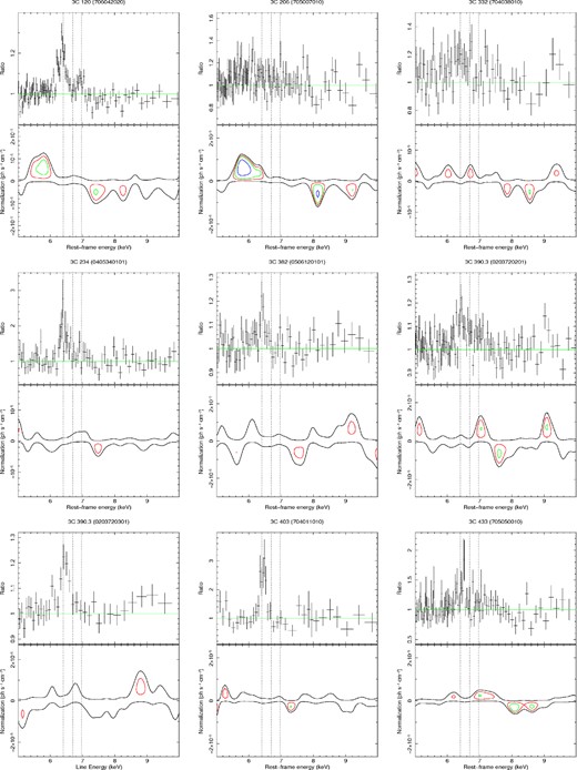
– continued
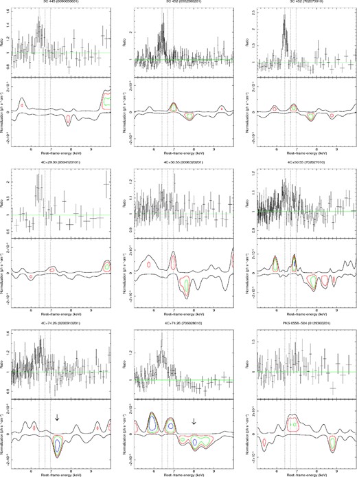
– continued
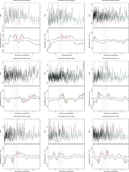
– continued
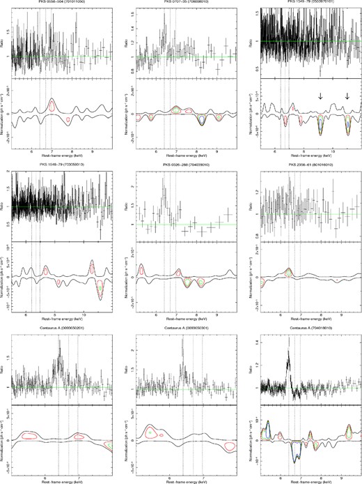
– continued
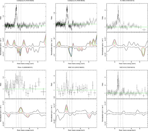
– continued
