


Abstract
Strong gravitational lensing can be used to directly measure the mass function of their satellites, thus testing one of the fundamental predictions of cold dark matter cosmological models. Given the importance of this test, it is essential to ensure that galaxies acting as strong lenses have dark and luminous satellites which are representative of the overall galaxy population. We address this issue by measuring the number and spatial distribution of luminous satellites in ACS imaging around lens galaxies from the Sloan Lens Advanced Camera for Surveys (SLACS) lenses, and comparing them with the satellite population in ACS imaging of non-lens galaxies selected from Cosmological Evolution Survey (COSMOS), which has similar depth and resolution to the ACS images of SLACS lenses. In order to compare the samples of lens and non-lens galaxies, which have intrinsically different stellar mass distributions, we measure, for the first time, the number of satellites per host as a continuous function of host stellar mass for both populations. We find that the number of satellites as a function of host stellar mass as well as the spatial distribution are consistent between the samples. Using these results, we predict the number of satellites we would expect to find around a subset of the Cosmic Lens All Sky Survey lenses, and find a result consistent with the number observed by Jackson et al. Thus, we conclude that within our measurement uncertainties there is no significant difference in the satellite populations of lens and non-lens galaxies.
1 INTRODUCTION
A key prediction of Λ cold dark matter (ΛCDM) is that galaxy-mass haloes should be surrounded by thousands of low-mass subhaloes. In apparent contrast to this prediction, only tens of companion satellite galaxies have been detected around the Milky Way (Strigari et al. 2007). This indicates that either ΛCDM is incorrect and the subhaloes do not exist, or that they do exist and do not form stars or retain sufficient amounts of gas to be detected (Papastergis et al. 2011). Even if future surveys such as Large Synoptic Survey Telescope (LSST) are able to detect a new population of ultrafaint dwarf galaxies around the Milky Way (e.g. Tollerud et al. 2008), the detection and study of these satellites outside of the Local Group would be unfeasible with present technology.
Therefore, a measurement of the subhalo mass function which is independent of star formation is necessary to confirm the accuracy of ΛCDM in this low-mass regime. There are several promising avenues for measuring the subhalo mass function in the Local Group, including direct detection of the annihilation of dark matter particles (Strigari 2013) and disruptions of tidal streams and the HI disk of the Milky Way by dark haloes (Carlberg, Grillmair & Hetherington 2012; Paardekooper, Khochfar & Dalla Vecchia 2013).
Outside of the Local Group, a powerful way to measure the subhalo mass function without relying on the presence of baryons is with strong gravitational lensing by a galaxy deflector. When a luminous background source is strongly lensed by an intervening galaxy, the number, positions and magnifications of the images that appear depend only on the mass distribution of the lens galaxy and the relative angular positions of the lens and the source (see Treu 2010, and references therein). Substructure along the line of sight can be identified via a deviation in the magnification, positions or time delays of lensed images from what would be expected given a smooth deflector mass distribution (e.g. Mao & Schneider 1998; Metcalf & Madau 2001; Keeton & Moustakas 2009).
Gravitational lensing has been applied to a variety of lens systems in order to detect subhaloes and place constraints on their mass function (e.g. Dalal & Kochanek 2002; Xu et al. 2009, 2013; Fadely & Keeton 2012; Vegetti et al. 2012). Due to the small numbers of systems available for this type of analysis, the uncertainties on the inferred subhalo mass function remain large. However, future wide-area surveys such as LSST and Panoramic Survey Telescope and Rapid Response System (PANSTARRS) are expected to find thousands of new lens galaxies (Oguri & Marshall 2010) which can be analysed for substructure. Furthermore, the next generation of large telescopes and adaptive optics will make the deep, high-resolution imaging required for the analyses of lensed images fast and therefore feasible for a large number of lenses, with sensitivity extending to lower masses.
In order to use the subhalo mass function measured around gravitational lenses as a test of ΛCDM, it is crucial to understand the lensing selection function, and in particular whether lens galaxies are representative of field galaxies. Several works have used simulations of different galaxy-scale lenses with background point sources to determine which dark matter halo properties and survey selection criteria affect the gravitational lensing cross-section (Keeton & Zabludoff 2004; Dobler et al. 2008; Mandelbaum, van de Ven & Keeton 2009; van de Ven, Mandelbaum & Keeton 2009; Arneson, Brownstein & Bolton 2012). These studies found that the lensing cross-section is by far most strongly dependent on the surface mass density of the deflector.
Treu et al. (2009) showed that lens galaxies in the Sloan Lens Advanced Camera for Surveys (SLACS) (Bolton et al. 2004, 2005, 2006; Auger et al. 2009) exist in environments with densities which are consistent with those of non-lens galaxies with similar stellar masses and velocity dispersions. Fassnacht, Koopmans & Wong (2011) found a similar result for a sample of intermediate-redshift lens galaxies. Furthermore, Auger et al. (2010) and Kochanek et al. (2000) showed that the Fundamental Plane for SLACS and Cosmic Lens All Sky Survey (CLASS; Browne et al. 2003; Myers et al. 2003) lens galaxies is consistent with that of non-lens, early-type galaxies.
In order to generalize the measurements of the subhalo population mass function of lens galaxies, it is essential that we understand whether lens galaxies have substructure populations typical of their non-lens counterparts. Outside of the Local Group, the comparisons between the subhaloes of lens and non-lens galaxies are only possible for those subhaloes which contain a significant population of stars. Those subhaloes which contain stars are expected to be the most massive, and therefore affect the lensing cross-section most strongly. We expect that the properties of the subhalo population which significantly alter the probability of lensing should be evident in the subhaloes containing luminous galaxies which are the most massive. Of course, with this sort of analysis, we cannot test whether there are indirect selection effects connecting lens galaxies and the dark subhalo population which do not directly influence the lensing cross-section.
As an important test, Jackson et al. (2010) counted the number of projected companions within 20 kpc apertures around lens galaxies in SLACS and CLASS, and compared them with the number of objects around early-type galaxies selected from Sloan and Cosmological Evolution Survey (COSMOS) ACS imaging. Jackson et al. (2010) found that SLACS lenses had a similar number of companion objects to other early-type galaxies in Sloan, while CLASS lenses had orders of magnitude more companions in projection than non-lens galaxies in COSMOS field galaxies.
In this work, we revisit the question of the populations of luminous companions of gravitational lenses, taking into account several important developments with regards to the detection and study of satellites. First, we apply the image processing and statistical analysis developed in Nierenberg et al. (2011, 2012, hereafter N11, N12) to ACS images of SLACS lenses, which enables us to directly study the satellite population of these galaxies to more than a thousand times fainter than the host galaxies and very close in projection (∼1.0 arcsec).
Secondly, we infer, for the first time, the dependence of the number of satellites on the host galaxy stellar mass for both SLACS lenses and COSMOS field galaxies. This allows us to rigorously incorporate differences in the distribution of host stellar masses when comparing between the two samples, which is essential given the strong observed dependence on the number of satellites as a function of host stellar mass (N12; Wang & White 2012).
The paper is organized as follows. In Section 2, we describe the selection of the sample of lens and non-lens host galaxies around which we study satellite galaxies. In Section 3, we describe our procedure for detecting companion objects around each of the samples of hosts. In Section 4, we explain the statistical method we use to infer the typical number of satellites per host galaxy as a function of stellar mass and redshift. In Section 5, we compare the inferred number of satellites per host for the SLACS and non-lens galaxies. In Section 6, we compare the number of satellites around COSMOS and CLASS hosts. Finally, in Section 7, we conclude with a discussion and summary of the results.
2 HOST GALAXY SELECTION
We restrict the galaxies analysed in this work to those which are imaged with sufficient depth and resolution to allow us to detect faint satellite galaxies. Furthermore, as the number of satellites is known to depend on the stellar mass of the host galaxy, we study only systems which had previously estimated stellar masses or multiple bands of photometry and a measured redshift, which enables us to estimate the stellar mass of the systems. Fig. 1 contains a summary of the redshift, stellar mass and apparent magnitude distributions of the host galaxies.
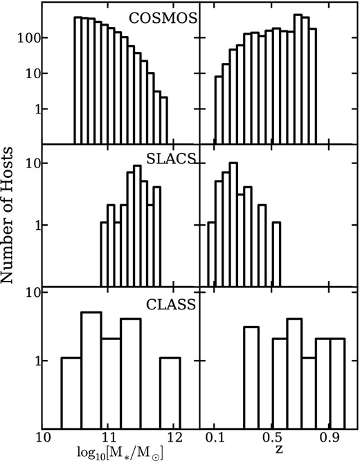
Stellar mass and redshift distributions of host galaxies considered in this work. Lens galaxies are systematically more massive than non-lens galaxies. This is expected given that the lensing cross-section increases as velocity dispersion to the fourth power.
2.1 Lens host galaxies
In this work, we focus mainly on measuring the properties of satellites around SLACS lens galaxies. SLACS candidates were detected in Sloan spectroscopy by searching for spectra which were composed of early-type, low-redshift lenses superimposed with a higher redshift emission-line galaxy. Lens status was then confirmed using either ACS or Wide Field Planetary Camera 2 (WFPC2) imaging to confirm the morphological characteristics expected in gravitational lensing (Bolton et al. 2004, 2005, 2006).
We restrict our comparison to those confirmed SLACS early-type lenses with redshifts z > 0.1 which have deep (multiple exposure) I814 imaging in order to enable us to measure the satellite population using the same tools which we apply to COSMOS imaging. We also require that the lenses were imaged with ACS rather than WFPC2, in order to ensure that there was a sufficient area of deep, high-resolution imaging around the lenses to allow for an accurate measurement of the satellite population. We excluded one system with detector artefacts very near the lens due to a saturated star, and one system which had four companions of comparable brightness in the field, making the detection of faint satellites impractical. The final sample contained 32 hosts. Host stellar masses, redshifts and photometry were obtained from Auger et al. (2010).
2.2 Non-lens host galaxies
We select non-lens host galaxies from the COSMOS ACS survey. We study host galaxies with stellar masses greater than M* > 1010.5 M⊙ as measured by Ilbert et al. (2010) using ground-based photometry in conjunction with ACS imaging (Auger et al. 2010). Hosts are restricted between redshifts 0.1 < z < 1 and to not within R200 of a more massive companion, where R200 is estimated using the observed relationship between stellar mass and R200 from (Dutton et al. 2010). This isolation requirement is included to ensure that we are not studying host galaxies which are themselves satellites of a more massive system. We also use the strong gravitational lensing catalogue by Faure et al. (2008) in order to exclude strong gravitational lenses from our sample.
COSMOS host stellar masses are based on SExtractor's MAGAUTO (Bertin & Arnouts 1996) from ACS imaging, unlike SLACS photometry which was performed using deVaucouleurs profile fitting. However, for bright galaxies, we found that this did not make a difference in COSMOS photometry (see also Benítez et al. 2004).
3 COMPANION DETECTION
We use the same method to detect companion objects around SLACS and COSMOS host galaxies as was used by N11 and N12. Briefly, the host galaxy light is modelled and removed from a cutout of ∼20 reff around the I814 images of host galaxies, using a modified version of the radial b-spline fitting code originally developed by Bolton et al. (2005, 2006). This method greatly facilitates the detection of nearby faint companions (see N11; N12). Once the host light has been subtracted, we use SExtractor to detect nearby objects with parameters tuned to match the detection rate and photometry of the publicly available COSMOS ACS photometric catalogues.1 We use masks of the lensed images created by the SLACS team (Auger et al. 2010) to define a minimum radius outside of which we search for companion objects, thereby ensuring that lensed images were not included in the final catalogue.
For COSMOS host galaxies, we compare our detections to those detections already in the COSMOS ACS photometric catalogues. New detections are added, while we replace the photometry for objects which were already in the photometric catalogues within ∼20 reff of the host galaxies with our own, thereby ensuring that the host light does not contaminate nearby objects.
For SLACS, we detect objects in the full ACS images around the lens galaxies and then add the new detections from the subtracted cutouts in the same way we do for COSMOS. For the SLACS images, bright stars and detector artefacts were masked by hand.
For both CLASS and SLACS hosts, we study all objects with I814 < 25 mag AB.
4 INFERENCE OF THE NUMBER OF SATELLITES PER HOST
Our data consist only of single-band photometry, so in order to study the properties of the satellite population, we use the statistical method developed by N11 and N12, which we briefly review here. This method relies on the fact that the properties of the number density signal of background/foreground objects and satellite galaxies have different radial dependences relative to central host galaxies, allowing us to jointly infer the properties of the spatial distribution and the numbers of background/foreground objects and satellite galaxies around a sample of host galaxies.
The statistical model can be summarized as follows: we infer the number of satellites per host within a fixed magnitude offset by modelling the spatial distribution of the number density signal near host galaxies as a combination of a homogenous background, with some mean value Σb, o, and number counts slope |$N_{\rm b}(<\!m_{{\rm max}})\propto 10^{\alpha _{\rm {b}}(m_{\rm {h},i}+{\rm dm}-m_{{\rm max}})}$| and a satellite population which has a projected radial distribution given by |${P}(r)\propto r^\gamma _{\rm p}$|, and an average number of satellites per host Ns, o. For simplicity, we do not consider the angular distribution of satellites in this work.
In this work, we include two new additions to the model which allow for an accurate comparison between samples of host galaxies with different stellar mass distributions and uncertain virial radii. We conclude by describing the priors used for the model. The likelihood function and a more detailed description of the statistics, including how we adjust for masked regions in the images can be found in Appendix A.
4.1 Number of satellites as a function of host stellar mass
This redshift evolution term in the foreground/background number density is not necessary for SLACS which covers a much smaller redshift range than the COSMOS hosts. We do not study redshift evolution in the number of satellites per host as there was no strong dependence apparent in N12.
4.2 Uncertainty in the virial radius
In order to account for variations in host halo mass and projected angular sizes due to redshift variations, it is important to choose an appropriate distance scale within which to study the satellite population. In N12, we scaled all distances by R200 as estimated by the observed relationship between stellar and halo mass from Dutton et al. (2010). This relationship becomes increasingly uncertain for high stellar masses (e.g. Behroozi, Conroy & Wechsler 2010).
The median stellar mass of the SLACS lens galaxies is |$\log [M^*_{{\rm host}}/{\rm M}_{\odot }]=11.4$|, which is approximately where the halo mass to stellar mass relation becomes very uncertain (e.g. Behroozi et al. 2010; Leauthaud et al. 2012). To account for this, for all hosts with stellar masses greater than |$\log [M^*_{{\rm host}}/{\rm M}_{\odot }]>11.4$|, the true virial radius is included as a model parameter, with mean and standard deviation given by Dutton et al. (2010). We further restrict the inference to only allow for virial masses Mvir < 1014 M⊙, as there are no clusters in either the COSMOS or SLACS samples, given group richnesses and lensing profiles. For our final results, we marginalize over the inferred virial radii. We note that the exact threshold where virial mass uncertainty is included does not significantly affect our results, as at lower stellar masses the stellar mass to virial mass uncertainty becomes smaller and the uncertainty due to the significantly smaller number of satellites per host dominates.
4.3 Priors
We use Gaussian priors on the parameters describing the number density of background/foreground objects (Σb,o, κb and δz, b). We obtain these priors by measuring the background properties in annuli between 1.0 < r < 1.5 R200 around the COSMOS hosts. For SLACS, we use priors with the same means as in COSMOS, but with broader standard deviations to allow for the fact that the COSMOS field is on average denser than pure-parallel fields (Fassnacht et al. 2011). We do not allow for redshift variation in the background/foreground number density in SLACS due to the small sample size and narrow redshift range of the central galaxies.
For COSMOS satellites, we apply a prior on the slope of the projected radial profile of γp from N12. Values for mean and standard deviations for these priors are listed in Table 1. We infer the properties of SLACS satellites with and without this prior on γp.
Priors used in the inference of the number and spatial distribution of satellite galaxies around SLACS and COSMOS host galaxies.
| Parameter | Description | COSMOS Prior | SLACS Prior |
|---|---|---|---|
| Ns,o | Number of satellites for hosts with M* = 1011.4 M⊙ | U(0,100)a | U(0,100) |
| κs | Dependence of satellite number on host stellar mass | U(0,60) | U(0,60) |
| γp | Projected radial slope of the satellite number density | N(−1.1,0.3)b | U(−9,0) |
| Σb,o | Number of background/foreground objects per arcmin2 with I814 < 25 | N(47,0.3) | N(47,2) |
| αb | Slope of the background/foreground number counts as a function of magnitude | N(0.300,0.005) | N(0.3,0.1) |
| κb | Dependence on the number of background/foreground objects on host stellar mass | N(1.5,0.3) | N(1.5,0.3) |
| δz, b | Dependence on the number of background/foreground objects with redshift. | N(0.03,0.02) | – |
aUniform prior between (min,max). bNormal prior with (mean, standard deviation).
We infer all parameters in bins of magnitude offset between companion and host galaxy (Δm = msat − mhost).
5 RESULTS
In Tables 2 and 3, we present the results of our inference on the cumulative number of satellites per host galaxy as a function of stellar mass and host redshift, in two bins of magnitude offset between host and companion objects Δm = msat − mhost.
Summary of inference results for SLACS satellites, see equations (1) and (2). Inferred between 0.03 < R < 0.5 R200.
| Δm | Ns,o | κs | γp | Σb, o | αb | Ns,oa | κsa |
|---|---|---|---|---|---|---|---|
| 4 | 6|$^{+3}_{-3}$| | 2.1|$^{+1}_{-0.7}$| | −0.7|$^{+0.2}_{-0.3}$| | 47|$^{+2}_{-2}$| | 0.38|$^{+0.05}_{-0.04}$| | 3|$^{+2}_{-2}$| | 3|$^{+1}_{-1}$| |
| 5 | 9|$^{+5}_{-3}$| | 2.4|$^{+1}_{-0.8}$| | −0.8|$^{+0.2}_{-0.3}$| | 47|$^{+2}_{-2}$| | 0.36|$^{+0.04}_{-0.02}$| | 7|$^{+3}_{-3}$| | 2.8|$^{+1}_{-0.9}$| |
| 6 | 20|$^{+5}_{-4}$| | 2.7|$^{+0.5}_{-0.5}$| | −0.7|$^{+0.1}_{-0.1}$| | 47|$^{+2}_{-2}$| | 0.39|$^{+0.02}_{-0.02}$| | 18|$^{+4}_{-4}$| | 2.7|$^{+0.7}_{-0.6}$| |
| 7 | 28|$^{+7}_{-6}$| | 2.7|$^{+0.5}_{-0.5}$| | −1.0|$^{+0.1}_{-0.2}$| | 46|$^{+2}_{-2}$| | 0.39|$^{+0.02}_{-0.02}$| | 27|$^{+5}_{-5}$| | 2.7|$^{+0.5}_{-0.5}$| |
| 8 | 37|$^{+9}_{-7}$| | 3.4|$^{+0.7}_{-0.5}$| | −1.0|$^{+0.1}_{-0.2}$| | 42|$^{+2}_{-2}$| | 0.39|$^{+0.02}_{-0.02}$| | 38|$^{+7}_{-7}$| | 3.5|$^{+0.6}_{-0.6}$| |
aInferred with a Gaussian prior on γp with mean −1.1 and standard deviation 0.3.
Summary of inference results for COSMOS satellites inferred between 0.03 < r < 0.5 R200, see equations (1) and (2).
| Δm | Ns,o | κs | γp |
|---|---|---|---|
| 2 | 0.8|$^{+0.2}_{-0.2}$| | 1.4|$^{+0.3}_{-0.3}$| | −1.1|$^{+0.1}_{-0.1}$| |
| 3 | 1.7|$^{+0.3}_{-0.3}$| | 1.7|$^{+0.3}_{-0.3}$| | −1.2|$^{+0.1}_{-0.1}$| |
| 4 | 2.9|$^{+0.4}_{-0.4}$| | 1.6|$^{+0.3}_{-0.2}$| | −1.1|$^{+0.1}_{-0.1}$| |
| 5 | 4.2|$^{+0.7}_{-0.8}$| | 1.8 |$^{+0.4}_{-0.3}$| | −1.1|$^{+0.1}_{-0.1}$| |
| 6 | 12|$^{+1}_{-1}$| | 2.3|$^{+0.4}_{-0.3}$| | −0.6|$^{+0.1}_{-0.1}$| |
| 7 | 20|$^{+3}_{-3}$| | 1.8|$^{+0.5}_{-0.5}$| | −0.8|$^{+0.2}_{-0.2}$| |
The results can be summarized as follows. For both COSMOS and SLACS hosts, we detect a significant dependence of the number of satellites per host on the host stellar mass, which is consistent between the samples. These results are also consistent with the results of N12, in which we observed that the number of satellites per host at fixed Δm was significantly higher for hosts with |$11<\log [{M^*_{\rm host}}/{\rm M}_{\odot }]<11.5$| than for hosts with |$10.5<\log [{M^*_{{\rm host}}}/{\rm M}_{\odot }]<11$|.
We find that the slope of the power-law radial profile of the satellite number density of satellites around SLACS lenses is consistent with that of COSMOS field galaxies and goes approximately as γp ∼ −1. As discussed by N11 and N12, this slope is approximately isothermal. Given the range of host concentrations across our sample, and the fact that we are fitting only a single power law to the radial profile of satellites, this result can be reproduced by a sum of Navarro, Frank and White radial profiles (Navarro, Frenk & White 1996) for the satellite number density, which is approximately the density profile which would be expected if satellite galaxies followed the density profile of the host halo, as predicted by simulations (e.g. Kravtsov 2010).
Therefore, we perform the inference a second time for SLACS galaxies using the same Gaussian prior on the projected radial profile as was used for COSMOS. These results are listed in the last two columns of Table 2. The Gaussian prior lowers the uncertainty in the inferred number of satellites, but it does not significantly affect the number of satellites per host.
In Fig. 2, we compare the inferred number of satellites for COSMOS and SLACS hosts using the same prior on γp. The number of satellites as a function of host stellar mass is consistent at all stellar mass values, although there may be a small trend in a steeper slope for the SLACS satellites, the difference is significant only at the ∼1σ level. Note that although values of individual parameters are not always consistent for COSMOS and SLACS, the average number of satellites as a function of host stellar mass is due to degeneracies between the parameters κs and Ns,o, and the final number of satellites as a function of stellar mass. In Fig. 3, we show the bivariate posterior probability distributions for κs and Ns, o for Δm = 4 and 7.
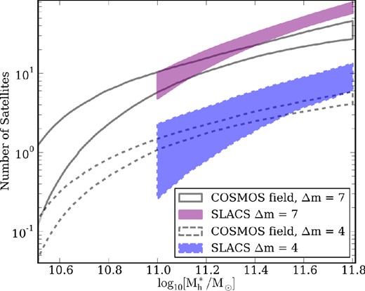
The average cumulative number of satellites per host within the range 0.03 < R200 < 0.5, near COSMOS and SLACS hosts, for two values of Δm where all objects analysed are restricted to have mobj − mhost < Δm. The filled curves show the 1σ confidence intervals for the inferred number of satellites per host as a continuous function of the host stellar mass. The inferred values for these functions are listed in Table 3. These results are inferred with a Gaussian prior on the projected slope of the satellite radial profile γp with mean −1.1 and standard deviation 0.3.
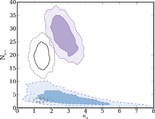
Comparison between posterior probabilities for the parameters κs and Ns,o for Δm = 4 and 7, for SLACS and COSMOS host galaxies. The colours have the same meaning as in Fig. 2. The darker inner contours and the lighter outer contours represent the 68 and 95 per cent confidence intervals, respectively.
6 COMPARISON WITH CLASS
Although the focus of this work is with the satellite population of SLACS lenses, it is interesting to see whether the CLASS lenses have a relatively higher rate of companion detection than COSMOS galaxies, given the stellar mass distribution of CLASS hosts and the results for our inference on the dependence between satellite number and host stellar mass.
Gravitational lenses in the CLASS (Browne et al. 2003; Myers et al. 2003) were selected by searching for flat-spectrum radio sources with multiple spatial components. This selection is very distinct from the SLACS selection, as it is purely based on the detection of a gravitationally lensed radio source, and has no requirements for the detection of the deflector galaxy. For this reason, the CLASS galaxies span a much larger range in redshift space than SLACS galaxies, and they do not all have well-measured photometry or redshifts. For this comparison, we consider only CLASS hosts which have I814 imaging with either WFPC2 or ACS2 and spectroscopic redshift measurements.
We obtained stellar masses of the CLASS lenses by compiling photometry from the literature (Muñoz et al. 1998; Rusin & Kochanek 2005; Lagattuta et al. 2010), and applying the stellar population synthesis modelling code by Auger et al. (2010). Due to the non-uniform methods of obtaining photometry across the different works, we assume a factor of ∼2 uncertainty in estimated stellar masses. We further restrict our sample to those lenses which have estimated stellar masses greater than M*/M⊙ > 1010.4 in order to allow us to continue using the functional form from equation (1). The final comparison sample consists of 14 hosts3 with properties shown in Fig. 1.
We use companion object detection from Jackson et al. (2010) who used SExtractor to detect objects within 20 kpc of the CLASS deflectors, with an I814 magnitude limit of 24.9. Jackson et al. (2010) visually excluded lensed images to ensure they were not counted as companion objects. After these considerations, Jackson et al. (2010) detect four companion objects within 20 kpc of the 14 CLASS host galaxies which have spectroscopic redshift measurements and meet our stellar mass requirements.
Using the stellar mass distribution of the CLASS hosts, we apply the results from the previous section to estimate the number of companion objects we would have expected around COSMOS hosts with the same stellar mass distribution. To do this, we drew randomly ten thousand times from the posterior probability distribution functions for κs, γp and Ns,o, as well as from Gaussian distributions centred on the estimated stellar masses with standard deviations of 0.3 dex in order to account for uncertainty in the host stellar mass estimates. We used the values of γp to rescale the expected number of satellites to the smaller area studied by Jackson et al. (2010).
Assuming that the closest satellites could be found only as close as 10 kpc, to the host centres, due to obscuration by the host galaxy, a sample of 14 COSMOS hosts with the same stellar masses and brightnesses as the CLASS hosts would have about 4 ± 2 satellites, and approximately 4 ± 2 background/foreground objects, depending on the assumed background/foreground number density around CLASS hosts. Given the small number statistics, this prediction is marginally consistent with the detection of four objects around CLASS hosts; however, these numbers do not take into account obscuration by lensed images.
We can roughly account for obscuration by lensed images, by assuming that the lensed images are found in annuli at the lens Einstein radii, with radial width of 0.4 arcsec. For double image lenses, we assume that about one third of the annulus is blocked by lensed images, and for four image lenses, we assume the full annulus is blocked, although the exact fraction of blocking does not significantly affect the results. Using this approximate accounting for lensed image obscuration, we expect 2–3 satellite galaxies and 1–2 foreground/background objects to be detected around CLASS host galaxies.
Although the main search radius in Jackson et al. (2010) was within 20 kpc, many of the companion objects around CLASS lenses were found even closer to the host galaxy, and brighter than the detection limit of 24.9. If we instead consider the number of objects between 4 and 14 kpc, within 3.3 mag of the central galaxy magnitude, our model would predict about two satellites and one background/foreground object, including the effects of obscuration which are less relevant this close to the central galaxy, in comparison with the four companion objects Jackson et al. (2010) detected which met these criteria.
Therefore, taking into account the fact that the CLASS host galaxies are very massive, we find that they have approximately the same number of nearby companion objects as we observe around COSMOS host galaxies with comparable stellar masses. This result highlights the importance of considering host stellar masses when comparing samples of satellite galaxies.
7 SUMMARY
We have measured the spatial distribution and number of satellites per host as a function of host stellar mass for SLACS lens galaxies and COSMOS field galaxies using host light subtraction, object detection and an updated version of the statistical analysis developed by N11 and N12. Furthermore, we compared the number of projected companion objects found within 20 kpc apertures of CLASS lens galaxies by Jackson et al. (2010) to what we would have expected around COSMOS field hosts with similar stellar masses.
Our main results are summarized below.
We detect a significant population of luminous satellites around SLACS lens galaxies. Parametrizing the spatial distribution of satellites as |$P_{{\rm sat}}(r)\propto r^{\gamma _{{\rm p}}}$|, we find γp ∼ −0.8 ± 0.2, which is consistent with the spatial distribution of luminous satellites around COSMOS non-lens galaxies.
Parametrizing the number of satellites per host within a fixed magnitude offset from the host galaxy (Δm = msat − mhost) to be |$N_{\rm {s}} \propto N_{\rm {s,\!o}}(1+{\rm \log _{10}[M^*_{{\rm host}}/{\rm M}_{\odot }]} - 11.4)^{\kappa _{\rm s}}$|, we find κs to be ∼2.9 ± 0.6 for SLACS satellites as measured for hosts between |$10^{11}<\log _{10}[M^*_{{\rm host}}/{\rm M}_{\odot }]<10^{11.8}$|, and ∼1.8 ± 0.5 for COSMOS satellites as measured between |$10^{10.5}<\log _{10}[M^*_{{\rm host}}/{\rm M}_{\odot }]<10^{11.8}$|. Given degeneracies between κs and Ns, o, the number of satellites per host as a function of host stellar mass is consistent within the measurement uncertainties for all values of Δm.
Using the above results, we find that the number of close companions to CLASS lenses found by Jackson et al. (2010) is consistent with what we observe around COSMOS non-lens galaxies, taking the distribution of CLASS host stellar masses into account, as well as obscuration due to bright lensed images.
From these results we conclude that the subhalo mass function measured from these strong gravitational lenses is representative of the global subhalo mass function for haloes of the same masses.
AMN, DO and TT acknowledge support from the Packard Foundations through a Packard Research Fellowship. AMN and DO also thank the Worster family for their research fellowship. We sincerely thank A. Sonnenfeld for estimating stellar masses of CLASS lenses, and B. Kelly, C. Fassnacht, N. Jackson and the anonymous referee for extremely helpful comments and discussions. This work was based on observations made with the NASA/ESA Hubble Space Telescope, and obtained from the data archive at the Space Telescope Science Institute, which is operated by the Association of Universities for Research in Astronomy, Inc., under NASA contract NAS 5-26555. These observations are associated with the COSMOS and Great Observatories Origins Deep Survey (GOODS) projects.
Packard Fellow.
COSMOS photometric catalogues and surveys are available at http://irsa.ipac.caltech.edu/data/COSMOS/datasets.html.
With the exception of 1422 which has I791 imaging.
CLASS B0128+437, MG0414+0534, CLASS B0445+123, CLASS B0631+519, CLASS B0712+472, CLASS B1030+074, CLASS B1152+199, CLASS B1422+231, CLASS B1608+656, CLASS B1933+503, CLASS B1938+666, CLASS B2045+265, CLASS B2108+213 and CLASS B2319+051
REFERENCES
APPENDIX A: LIKELIHOOD FUNCTION
Here, we describe how we infer the model parameters |$\boldsymbol {\theta }$| (listed in Table 1), which describe the number and spatial distribution of satellite and background/foreground galaxies between 0.03 and 0.5 R200 as a function of host stellar mass, within a fixed magnitude offset from the host galaxy (mobj − mhost < Δm), given our data |$\boldsymbol {D}$|.
