


Abstract
Low-mass star-forming regions are more complex than the simple spherically symmetric approximation that is often assumed. We apply a more realistic infall/outflow physical model to molecular/continuum observations of three late Class 0 protostellar sources with the aims of (a) proving the applicability of a single physical model for all three sources and (b) deriving physical parameters for the molecular gas component in each of the sources. We have observed several molecular species in multiple rotational transitions. The observed line profiles were modelled in the context of a dynamical model which incorporates infall and bipolar outflows, using a three-dimensional radiative transfer code. This results in constraints on the physical parameters and chemical abundances in each source. Self-consistent fits to each source are obtained. We constrain the characteristics of the molecular gas in the envelopes as well as in the molecular outflows. We find that the molecular gas abundances in the infalling envelope are reduced, presumably due to freeze-out, whilst the abundances in the molecular outflows are enhanced, presumably due to dynamical activity. Despite the fact that the line profiles show significant source-to-source variation, which primarily derives from variations in the outflow viewing angle, the physical parameters of the gas are found to be similar in each core.
1 INTRODUCTION
The astrophysical mechanism of gravitational infall coupled with rotation and axisymmetric outflows operates on a vast range of scales, ranging from black holes and jets in active galactic nuclei (such as M87) through to high- and low-mass star formation (Livio 2004) and even brown dwarfs (Whelan et al. 2007).
Searches for the signatures of the early stages of star formation have tended to focus on infall indicators in Class 0 low-mass protostellar objects. These possess a luminous protostellar core, but – by definition – most of the mass is contained in a surrounding envelope. In most models, the fraction of the mass in the envelope that is infalling increases with time (e.g. Shu, Adams & Lizano 1987). In the early stages, the gas is approximately isothermal, and the envelope can be approximated by a spherically symmetric hydrostatically supported cloud. Emission from the envelope includes regions where the gas is infalling and where it is static.
In these circumstances, the classic observational signature of infalling optically thick molecular gas is a double-peaked asymmetric line emission profile (Zhou et al. 1993). Molecular emission lines originating from quiescent gas residing in the outer parts of the envelope have line widths consistent with thermal contributions alone as opposed to thermal and turbulent line broadening of dynamic gas (Keto et al. 2004).
However, collapse seems to almost always lead promptly to disc, jet and (bipolar) outflow formation. These outflows arise because molecular gas in the envelope is entrained by protostellar jets. The latter are hot, high-velocity (∼200 km s−1) jets of mostly atomic hydrogen that carry away excess angular momentum from the core. It is difficult to isolate the cases of clouds on the verge of collapse and in such cases local turbulent or global oscillations can mask the weak initial collapse motions (Lada et al. 2003; Redman, Keto & Rawlings 2006; Gao & Lou 2010). Once collapse is clearly present, line profile shapes become complex and ambiguous. The classic blue-asymmetric line profile shape that can indicate collapse can also be generated by other large-scale dynamical effects such as rotation (Redman et al. 2004) or outflows (Rawlings et al. 2004). Moreover, whilst dynamic processes alter spectral line profiles, they are also affected by chemical processes which change the molecular abundance, thereby altering the line intensity. These chemical processes include gas-phase reactions, the freeze-out of molecular gas on to dust grains (Schöier et al. 2002) in the cold, dense envelope and the desorption of molecular gas in the warmer outflow regions (Wiseman et al. 2001).
To investigate infall, the presence of other effects should be accounted for. This is not possible with one-dimensional radiative transfer codes because only radial motions can be modelled. Two-dimensional codes are useful because many systems will have cylindrical symmetry around the outflow axis. In fact, the line profile observed from a molecular outflow changes dramatically as the angle varies between the outflow axis and the observer's line of sight (Ward-Thompson & Buckley 2001). To allow for an arbitrary viewing angle relative to the symmetry axis, it is therefore necessary to couple the 2D codes to 3D ray-tracing algorithms. Specific sources may exhibit significant deviations from axisymmetry. These could arise, for example, if the outflows are non-axisymmetric and/or there is significant non-symmetric structure in the envelope or circumstellar disc. In these cases, a fully three-dimensional approach is required. The drawback of 3D codes is that they have large memory requirements for fine grid resolution.
In this paper, we continue our coupled observational and modelling investigation of early stage collapse objects that are clearly undergoing dynamical activity and harbour a central accreting source. We analyse the emissions from a sample of three low-mass protostellar cores which possess evidence of both infall and outflows. The line profiles of several molecular line transitions are observed which effectively probe the conditions in the dense core, diffuse envelope and molecular outflow. These are used to characterize the physical parameters (such as the temperatures, densities and chemical abundances) of each source in the context of a single unified dynamical model that includes infall and a bipolar outflow. To do this, we have utilized a 3D radiative transfer code, MOecular LIne Explorer (mollie; Keto et al. 2004) that is specifically employed to study how the line profiles are constrained by the orientation of the outflow axis with respect to the observer.
We aim to show that a single unified model, comprising a spherically symmetric envelope/inflow and a bipolar outflow with a narrow interface region, can be used to describe the emission from each source. We further wish to test the hypothesis that the significant source-to-source variations that are observed are primarily the results of differences in the source orientation/viewing angle.
Different isotopologues and transitions of the same molecular species preferentially trace somewhat different physical conditions within a dynamically active core. For example, an outflow may be best observed in a low-excitation transition of an abundant transition such as the 12CO or 13CO line whereas the envelope turbulent velocity may be better constrained by the hyperfine structure in, for example, the C17O lines. The source models were assembled by first modelling the different dynamical components, using the transition in which they are most strongly apparent. Then, using this information, a self-consistent model for the entire source was constrained using all species and transitions.
Section 2 summarizes the properties of the sources and Section 3 describes our continuum/molecular observations used to constrain the modelling. Section 4 introduces the mollie code and our method, analysis, and the results obtained are given in Section 5. Section 6 discusses these results and our concluding remarks are given in Section 7.
2 SOURCES
Our study concentrates on three protostellar cores: B335, I04166 and L1527, which are each believed to be in the Class 0 phase of evolution for low-mass protostellar objects. They have similar spectral energy distributions (SEDs) and, being of a similar evolutionary status, should be described by a single physical model.
Extensive observational data (molecular and continuum) and modelling efforts already exist for these sources and, significantly, spectral signatures of both infall and outflow are seen to be present. We therefore hope to be able to identify the similarities and the source-to-source variations that exist within objects at a similar evolutionary stage.
As an example of the types of variations that are observed, Fig. 1 presents the 13CO J = 2–1 line profiles at the zero offset (0,0) position for each of the cores. Significant variations in profile shape and strength are clearly evident.
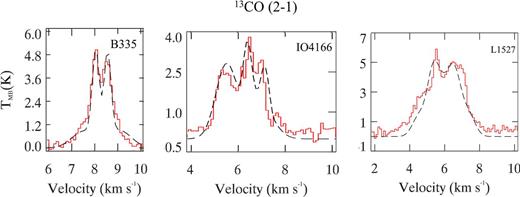
13CO (J = 2-1) line profiles at the (0, 0) offset position for B335, IO4166 and L1527.
We briefly summarize here the key points from some previous studies, relating to the morphology and dynamical structure of each source.
2.1 B335
B335 is a very well studied core (Hodapp 1998; Wilner et al. 2000; Evans et al. 2005; Stutz et al. 2008; Yen, Takakuwa & Ohashi 2010, 2011) located 250 pc away (Tomita, Saito & Ohtani 1979) and contains the IRAS source 19347 + 0727 (Huard, Sandell & Weintraub 1999).
It is, to a large extent, the prototypical Class 0 infall source in that it was the first such object in which the classic asymmetric double-peaked infall line profiles were identified and analysed (Zhou et al. 1993). This analysis was helped by the fact that it is isolated, singular and approximately spherical. In addition, the outflow lobes are approximately in the plane of the sky, minimizing the dynamical confusion between infall and outflows.
The infall component was detected through the observation of several transitions in both single-dish and interferometric modes (Chandler & Sargent 1993; Zhou et al. 1993; Velusamy, Kuiper & Langer 1995; Nisini et al. 1999). The clear presence of infall, coupled with the existence of a massive envelope gas, indicates significant accretion and is consistent with a Class 0 protostellar object (André, Ward-Thompson & Barsony 1993).
Monte Carlo radiative transfer modelling by Choi et al. (1995) was successful in describing the observed line emission towards the centre of the molecular cloud in the context of the well-known spherically symmetric ‘inside-out’ collapse model of Shu (1977). An infall (‘collapse expansion wave’) radius of 0.035 pc was deduced (Zhou et al. 1993). The expected density profile within the free-fall zone (∝r−1.5) is consistent with near-infrared extinction maps by Harvey et al. (2001). Outside the infall radius, the density profile is consistent with that expected for a static singular isothermal sphere (Saito et al. 1999; Shirley et al. 2000).
Emission from a bipolar molecular outflow was observed in molecular line spectra by Moriarty-Schieven & Snell (1989). The outflow is very close to the plane of the sky (∼10°) and is elongated in the east–west direction (Cabrit, Goldsmith & Snell 1988; Hirano et al. 1988; Saito et al. 1999).
2.2 I04166
I04166 is a protostellar object located in the Taurus molecular cloud at a distance of 140 pc (Elias 1978) and contains the IRAS source 04166 + 2706 (Kenyon et al. 1990). The radius of the molecular gas cloud has been estimated from the extent of molecular line emission from the high-density tracers NH3 (1,1) and (2,2) and from 1.2 mm continuum emission. Both are coincident out to a distance of 0.03 pc (Tafalla et al. 2004). Motte & André (2001) constructed an SED which is consistent with a Class 0 source, and observations of N2H+ (J = 1-0) by Chen, Launhardt & Henning (2007) inferred a mean molecular hydrogen number density, |$n_{\rm H_{2}} = 4 \times 10^{6}$| cm−3.
I04166 contains a highly collimated molecular outflow. The axis position angle is 30° (east of north) and extends 0.25 pc either side of the IRAS source (Bontemps et al. 1996). Tafalla et al. (2004) observed the outflow in 12CO (J = 2-1) emission and found there are two distinct velocity components, one is at 50 km s−1 and a slower component with a velocity <10 km s−1. A faster gas component is usually associated with the youngest of protostellar objects (Bachiller 1996). The slow gas is believed to be created by a shear flow of accelerated ambient gas moving along the wall of an evacuated cavity.
2.3 L1527
Like I04166, L1527 is a protostellar core located in the Taurus molecular cloud at a distance of 140 pc and it contains the IRAS source 04368 + 2557 (Elias 1978). Double-peaked asymmetric line spectra consistent with gravitationally infalling gas were observed by Zhou et al. (1994) and Myers et al. (1995). Observations by Zhou, Evans & Wang (1996) and radiative transfer modelling by Myers et al. (1995) determined an infall radius of 0.03 pc. Continuum observations from 100 → 800 μm shows that the gas density profile varies as r−1.5 within a radius of 0.03 pc. An upper limit to the age of this source was calculated by Ohashi et al. (1997) to be 105 yr on the assumption of a constant accretion rate. However, Kenyon et al. (1993) found that a fit to the SED gives a lower age of 4.6 × 10³ yr indicating that this is a young Class 0 source (André et al. 1993).
A molecular outflow was observed in single-dish and interferometric observations by MacLeod, Avery & Harris (1994) and Tamura et al. (1996). The outflow emission has an hourglass morphology (Zhou et al. 1996; Ohashi et al. 1997) with the outflow axis at <10° to the plane of the sky (Tamura et al. 1996).
More recent Spitzer observations of L1527 have clearly revealed the bipolar outflow structure but have also identified the presence of a ‘dark lane’ which has been ascribed to a modified inner envelope/outflow cavity morphology (Tobin et al. 2008). This inner ‘nozzle’ has a distinct effect on the Spitzer and near-infrared images of the source, but the scale of the structure (∼100 au) is such that it would not significantly affect line profiles as observed at single-dish resolution.
3 OBSERVATIONS AND DATA
Line observations of our sources were made with the James Clerk Maxwell Telescope (JCMT) over a period of 18 months (mostly in service mode) using heterodyne receivers. We obtained a variety of strip and five-point maps for the various sources/transitions that we have considered, which have given sufficient data coverage of our sources so as to allow accurate modelling. We have also used JCMT Submillimetre Common-User Bolometer Array (SCUBA) archival data for 450/850 μm continuum emission.
3.1 Molecular line observations
The cores were observed with RxA3 (and RxA2) in 2001 August and 2003 March–May. All observations were made in frequency switching mode and the details of the transitions are given in Table 1. The data were reduced using the specx software package and further analysis was undertaken with the class package. For the majority of the observations, the system temperature was between 300 and 450 K. A main beam correction factor of 0.69 was used to convert the antenna temperatures into TMB. The critical density for thermalization (ncrit) for each transition is also given in Table 1. These show the wide range of densities (9 × 10³-3 × 106 cm−3) that are probed by the chosen molecular tracers/transitions.
The observed line emission tracers modelled in this paper.
| Source | Molecule | Transition | ncrit (cm−3) | Receiver | Date observed |
|---|---|---|---|---|---|
| B335 | H13CO+ | (J = 3-2) | 3.4 × 10⁶ | A3 | 20 August 2001 |
| HCO+ | (J = 3-2) | 1.8 × 10⁶ | A2 | 18 February 1997 | |
| 13CO | (J = 2-1) | 9.6 × 10³ | A3 | 15 May 2003 | |
| C18O | (J = 2-1) | 9.5 × 10³ | A3 | 3 May 2003 | |
| C17O | (J = 2-1) | 1.0 × 10⁴ | A3 | 3 May 2003 | |
| I04166 | 13CO | (J = 2-1) | 9.6 × 10³ | A3 | 1 April 2003 |
| C18O | (J = 2-1) | 9.5 × 10³ | A3 | 18 March 2003 | |
| C17O | (J = 2-1) | 1.0 × 10⁴ | A3 | 3 May 2003 | |
| L1527 | H13CO+ | (J = 3-2) | 3.4 × 10⁶ | A3 | 3 May 2003 |
| 12CO | (J = 2-1) | 1.1 × 10⁴ | A3 | 3 May 2003 | |
| 13CO | (J = 2-1) | 9.6 × 10³ | A3 | 3 May 2003 | |
| C18O | (J = 2-1) | 9.5 × 10³ | A3 | 3 May 2003 | |
| C17O | (J = 2-1) | 1.0 × 10⁴ | A3 | 3 May 2003 |
3.2 Dust continuum observations
Archival SCUBA data of our three sources were retrieved and reduced using the surf package. The data consist of dust continuum emission observed at 850 and 450 μm. All our science observations are 64-point jiggle maps with a 120 arcsec chop throw. Wavelength-dependent submillimetre extinction, τ850 and τ450, were calculated from skydip observations. Bolometers at the edge of the array and those with excessive noise (Vrms ≥ 60 nV) were removed before the data were rebinned to 0.5 θMB per pixel on a J2000 coordinate system. The SCUBA emission maps were converted to jansky units using flux calibration factors (FCFs) calculated from photometry observations of Uranus. The FCFs for each source are listed in Table 2 for each source.
Flux calibration factors from photometry observations of Uranus. The calibration factors listed are determined for 40 and 120 arcsec beams. Emission maps at 450 and 850 μm of B335, L1527 and I04166 were originally published in Shirley et al. (2000).
| Source | α (J2000) | δ (J2000) | τ850 | τ450 | Date | FCF|$^{850}_{40}$| | FCF|$^{850}_{120}$| | FCF|$^{450}_{40}$| | FCF|$^{450}_{120}$| |
|---|---|---|---|---|---|---|---|---|---|
| (Jy V−1) | (Jy V−1) | (Jy V−1) | (Jy V−1) | ||||||
| B335 | 19 37 01.13 | 07 34 10.9 | 0.14 | 0.69 | 17 April 1998 | 1.01 | 0.86 | 5.84 | 3.98 |
| I04166 | 04 19 42.5 | 27 13 36 | 0.17 | 0.77 | 30 August 1998 | 0.98 | 0.77 | 5.32 | 3.74 |
| L1527 | 04 39 53.89 | 26 03 10.5 | 0.15 | 0.76 | 24 January 1998 | 1.02 | 0.92 | 5.76 | 5.34 |
4 MODELLING
4.1 The physical model
For the purpose of the radiative transfer modelling, we have used a simple dynamical model that is similar to that described in Rawlings et al. (2004). This is a multicomponent physical construct that includes a static envelope of molecular gas whose density varies with radius from the centre of the gas cloud and a bipolar outflow. The temperatures in the envelope and the outflow interface components are taken to be spatially invariant. This is obviously a significant simplification but, as shown in Tsamis et al. (2002), in the case of the low-J lines observed at low spatial resolution that we are modelling, the line profiles are generally more sensitive to abundance variations and the gas dynamics than they are to the temperature profile. Obviously, this assumption breaks down in the case of smaller beams and/or higher levels of excitation. It is assumed that the envelope and the outflow are dynamically decoupled from each other as the interactions between the two are most likely limited to narrow interface regions.
The outflow is driven by a high-speed, low-density hot jet which, through turbulent shear, accelerates the molecular gas. Within the outflow the temperature, velocity and density will vary with distance from the jet axis. Observations (e.g. Gueth & Guilloteau 1999) indicate that the highest velocity and most excited molecular gas is typically located in a narrow region close to the underlying jet. For convenience, the molecular outflow is divided into two regions, a hot, low-density inner region which is close to the protostellar jet (hereafter the ‘inner boundary layer’) and a denser, cooler region at the interface between the outflow envelope (hereafter the ‘outer boundary layer’). A better approximation would be a linear variation in the outflow parameters between the interface with the jet and with the envelope; however, due to the resolution of the single-dish observations being modelled, this refinement would result in little change to the line profiles. So, for simplicity, we employ a two-component molecular outflow model.
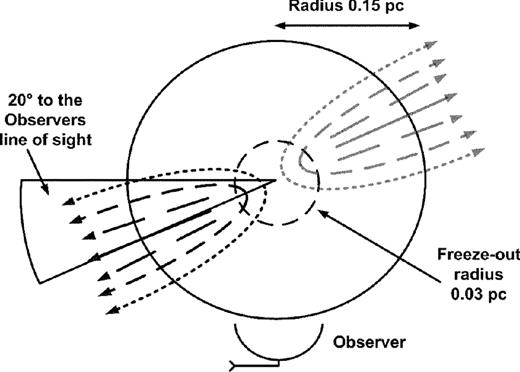
Schematic diagram of the dynamical model. The dashed line shows the outer boundary layer, the broken lines show the inner boundary layer and the solid line represents the unobserved underlying jet. The viewing angle (the tilt between the axis of the outflow lobes and the plane of the sky) and freeze-out radius are for I04166. The dynamical models for L1527 and B335 have different viewing angles and radii, recorded in Table 3.
4.2 Radiative transfer modelling
In order to interpret the observed line emission profiles, a thorough analysis of the spectra must account for the simultaneous processes of infall, outflow, gas freeze-out and desorption including the contributions to the profile formation at all points along the line of sight.
We have utilized a 3D radiative transfer code, mollie,1 written and developed by Keto and collaborators (see, e.g., Keto 1990; Keto et al. 2004; Redman et al. 2004, 2006; Carolan et al. 2008, 2009; Longmore et al. 2011 for examples of its use). mollie is used to generate synthetic line profiles to compare with observed rotational transition lines. In order to calculate the level populations, the statistical equilibrium equations are solved using an accelerated lambda iteration algorithm (Rybicki & Hummer 1991) that reduces the radiative transfer equations to a series of linear problems that are solved quickly even in optically thick conditions. mollie splits the overall structure of a cloud into a 3D grid of distinct cells.
The input to mollie is divided into voxels (3D pixels) and there are five input parameters which need to be uniquely defined for each voxel: the number density of H2, the gas temperature, the gas bulk velocity, the microturbulent velocity of the gas and the chemical abundance. As described in the next section, the parameters other than the abundance can each be constrained from the continuum and molecular observations, coupled with radiative transfer calculations.
Carolan (2009) calculated the chemical abundances in a detailed chemical model for simple spherically symmetric clouds and investigated the sensitivity of the resulting molecular line profiles to the chemical variations. He found that, because the largest chemical changes tend to take place in the centre of the cloud (as a result of molecular freeze-out), the CO abundance in the bulk of the volume of the cloud can be taken to be approximately constant. Again, we note that the line profiles convolved to the resolution of single-dish observations do not significantly resolve the chemical variations. Therefore, we have not performed any chemical modelling in this study, rather we use the observations to constrain the molecular abundance for each of the envelope, inner boundary layer and outer boundary layer in the sources.
Subsequently, we perform a chi-squared analysis to find the best-fitting parameters. This procedure works by running a series of simulations with the abundance kept constant whilst the other four parameters are varied. This is repeated for different abundances until a best fit is found (Carolan 2009).
5 ANALYSIS AND RESULTS
The chi-squared analysis described above can be used to obtain best-fitting parameters from an arbitrary first approximation but, wherever feasible, we try to simplify the procedure by using simple analyses of observational data to constrain as many of the free parameters as possible. These values are then refined by the modelling/chi-squared fitting analysis.
In practice, this is not possible for the outflow and interface components. However, in the case of the envelope, if we make the assumptions described above (spherical symmetry, density structure described by a Plummer law and isothermality), we can make some rough first estimates of the key physical parameters, using optically thin C18O (J = 2-1) line and/or dust continuum emission data.
Using this approach, we obtain constraints on the following quantities: (a) the characteristic radius within which the CO abundance is significantly reduced as a result of freeze-out on to dust grains, (b) a representative depletion factor, (c) the normalization (ρ0,R0) for the (Plummer) density profile, (d) the gas temperature and (e) the turbulent velocity. The (highly simplified) procedure that we adopt is as follows.
CO freezes out on to the surface of dust grains at low temperatures (T ≲ 20 K) and high densities (|$n_{\rm {H}_{2}} \gtrsim 10^{4}$| cm−3) (Sandford & Allamandola 1993). To determine the degree of freeze-out, we compare spatial distributions of the H2 column density as determined from the dust continuum observations to those determined from molecular (CO) observations. The offset between the two gives a measure of the amount of molecular depletion on the assumption that freeze-out is the only cause of the CO abundance reduction. The absolute normalization will depend on such factors as the dust opacity, the dust-to-gas ratio and the (assumed constant) CO:H2 ratio, and so is highly uncertain, but the relative variations across the core will be reasonably well defined.
The column density of H2 has also been determined from molecular gas observations using the optically thin rotational transition C18O (J = 2-1), with the simplifying assumptions of isothermality and a standard CO:H2 ratio. This analysis is fully described in Appendix A.
Fig. 3 shows comparisons between the two as observed in each of the three sources. The dust emission profiles closely match the results from previous studies (e.g. Shirley, Evans & Rawlings 2002). Each plot in Fig. 3 clearly shows the presence of depletion, which becomes more significant as one approaches the centre of each core. We simplify the complexity of this structure by a step function, so that a nominal depletion radius is defined for each source, within which the gas-phase CO abundance is reduced by a factor of between 3 and 10. These parameters are initially estimated from Fig. 3 and then further refined by the modelling/fitting technique.
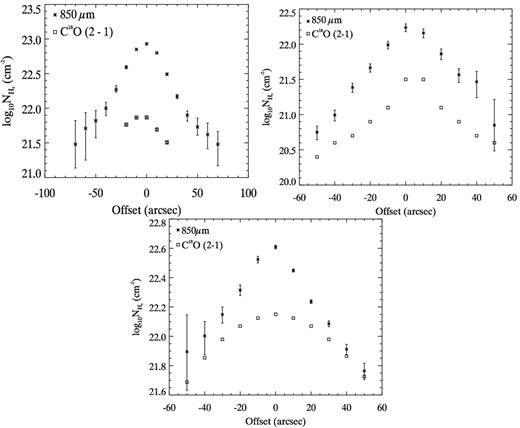
A comparison of the column density of H2 derived from SCUBA dust continuum and integrated C18O molecular line emission for B335, I04166 and L1527, respectively.
Using a Plummer law for the density profile and assuming spherical symmetry in the envelope, we then use the column densities of H2 derived from the (undepleted) dust continuum emission to determine the normalization factors (R0, ρ0) in equation (1) and hence the number density of H2: |$n_{{\rm H}_{2}}$|.
There are a couple of major assumptions with this method. (i) We assume that the dust and gas are well coupled, in which case a single value can be used to describe both the gas and the dust temperatures. For the dense cores that we are investigating, this is a fair approximation. (ii) We do not allow for any spatial variation in temperature across the envelope. Temperature structure is known to exist (e.g. Shirley et al. 2002), but the magnitude of those variations is not sufficient to warrant a more detailed approach in a simple model that is tailored to what can be detected at single-dish resolution.
5.1 Radiative transfer modelling of the observed spectral line emission
Our results and best-fitting parameters are described in this section for each of our three sources. Table 1 lists the molecular transition observed for each source, and the results are presented in Figs 4–16 with the observed emission line profiles overlaid with the best-fitting modelled profiles. The best-fitting model parameters are given in Tables 3–5. The number of significant figures given in these tables indicates the level of accuracy obtained by the chi-squared fitting technique.
B335: C17O (J = 2-1) line profiles – observed (solid line) and modelled (dashed line). The offset between cells is 10 arcsec.
Best-fitting parameters for the gas in the envelope of each source. The first eight parameters were roughly constrained by observations and then fine tuned to improve the model fits. The outflow tilt angle is relative to the plane of the sky and the abundance is the column density ratio relative H2.
| Envelope parameters | B335 | I04166 | L1527 | |
|---|---|---|---|---|
| Outflow tilt angle (°) | −10 | 20 | 10 | |
| Source radius | (pc) | 0.15 | 0.15 | 0.08 |
| Depletion radius | (pc) | 0.05 | 0.03 | 0.015 |
| CO depletion factor | 10 | 3 | 3 | |
| Temperature | (K) | 20 | 20 | 20 |
| Peak density | (cm−3) | 106 | 4 × 10⁶ | 106 |
| Velocity | (km s−1) | −0.3 | −0.2 | −0.3 |
| Turbulent width | (km s−1) | 0.25 | 0.2 | 0.3 |
| Abundance C17O | (×10−8) | 3.5 | 0.98 | 0.075 |
| Abundance C18O | (×10−8) | 30 | 2.6 | 0.30 |
| Abundance 13CO | (×10−8) | 180 | 6 | 5 |
| Abundance 12CO | (×10−8) | 400 | ||
| Abundance HCO+ | (×10−8) | 3 | ||
| Abundance H13CO+ | (×10−8) | 0.09 | 0.0022 |
Best-fitting parameters for the gas in the outer boundary layer. This corresponds to the molecular gas at the interface between the molecular outflow and the envelope. The first four parameters were constrained by observations and then fine tuned to improve the model fits. The abundances are relative to H2.
| Parameters in the outer | B335 | I04166 | L1527 | |
|---|---|---|---|---|
| boundary layer | ||||
| Temperature | (K) | 35 | 50 | 30 |
| Peak density | (cm−3) | 105 | 105 | 9 × 10⁴ |
| Velocity | (km s−1) | 1.4 | 1.2 | 1.3 |
| Turbulent width | (km s−1) | 0.3 | 0.4 | 0.4 |
| Abundance 13CO | (×10−8) | 300 | 10 | 60 |
| Abundance 12CO | (×10−8) | 450 | ||
| Abundance HCO+ | (×10−8) | 9 |
Best-fitting parameters for the gas in the inner boundary layer of each source. The inner boundary layer is the molecular gas in the outflow that is closest to the protostellar jet. The first four parameters were constrained by observations and fine tuned to improve the model fits. The abundances are relative to H2.
| Parameters in the inner | B335 | I04166 | L1527 | |
|---|---|---|---|---|
| boundary layer | ||||
| Temperature | (K) | 55 | 80 | 60 |
| Peak density | (cm−3) | 104 | 5 × 10⁴ | 104 |
| Velocity | (km s−1) | 3.5 | 1.6 | 2.5 |
| Turbulent width | (km s−1) | 0.5 | 0.6 | 0.6 |
| Abundance 13CO | (×10−8) | 600 | 12 | 400 |
| Abundance 12CO | (×10−8) | 600 | ||
| Abundance HCO+ | (×10−8) | 12 |
5.1.1 B335
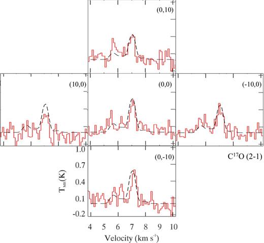
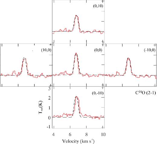
B335 was observed in several molecular species/transitions. Line profiles of the optically thin (J = 2-1) transition of C17O and C18O are shown in Figs 4 and 5. They are shown as a strip of spectral line profiles that are centred at the peak of 850 μm dust continuum emission which corresponds to the (0, 0) offset in both Figs 4 and 5.

B335: C18O (J = 2-1) line profiles – observed (solid line) and modelled (dashed line). The offset between cells is 10 arcsec.
The observed line emission profile of C17O (J = 2-1) arises from separate hyperfine line transitions whose peaks are clearly distinguishable in Fig. 4. In a highly turbulent gas, the components would be blended. The spectra of C18O (J = 2-1) are single peaked and have similar intrinsic line widths as the C17O (J = 2-1) lines. It would therefore seem that both transitions are preferentially probing cold, quiescent gas in the envelope. The best-fitting parameters from the radiative transfer modelling of the molecular gas envelope are listed in Table 3. Blanks in the table imply that the line profiles are insensitive to the abundances which are therefore unconstrained by the model.
The turbulent velocity in the envelope gas was calculated to be 0.25 km s−1, as determined from the C18O (J = 2-1) line profiles. To account for the observed molecular depletion, as evident in Fig. 3, the C18O (J = 2-1) and C17O (J = 2-1) line profiles were modelled with an abundance that is reduced by a factor of 10 inside a freeze-out radius of ∼0.3 times the core radius.
The best-fitting abundances of C18O obtained inside and outside the freeze-out region are 3 × 10⁻⁸ and 3 × 10⁻⁷, respectively. These are similar values to those obtained by Evans et al. (2005): 2.5 × 10⁻⁸ and 7.4 × 10⁻⁸. C17O was modelled with the same depletion factor so that the best-fitting abundances were 0.35 × 10⁻⁸ and 3.5 × 10⁻⁸. This implies a value for the 18O:17O ratio that is a factor of ∼2 larger than interstellar values (Schöier et al. 2002).
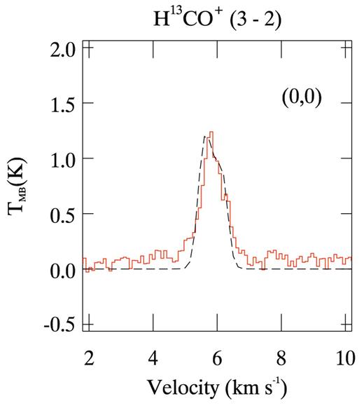
Fig. 6 shows the observed line spectra and the modelled profiles for HCO+ (J = 3-2). The observational data consist of a single line profile at zero offset. H13CO+ (J = 3-2) line profiles are shown in Fig. 7. Although clearly present in the zero offset position, there is barely any emission detected in the (20 arcsec) off-centre spectra. This is not surprising as the critical densities of the transitions are 1.8 × 10⁶ and 3.4 × 106 cm−3, respectively, larger than the peak H2 density in B335.
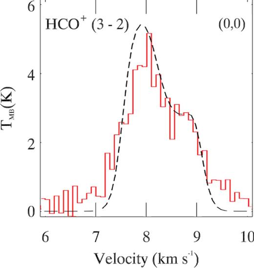
B335: HCO+ (J = 3-2) line profiles at the (0,0) offset position – observed (solid line) and modelled (dashed line).
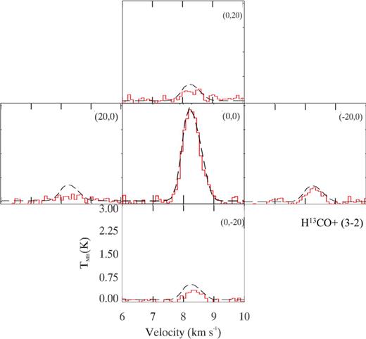
B335: H13CO+ (J = 3-2) line profiles – observed (solid line) and modelled (dashed line). The offset between cells is 20 arcsec and the middle panel is at the 0 arcsec offset.
The values of the temperature, peak density, infall and turbulent velocities were constrained from the C18O (J = 2-1) and C17O (J = 2-1) lines. The best-fitting HCO+ abundance is 3 × 10⁻⁸ which agrees well with the value (3.5 × 10⁻⁸) obtained by Evans et al. (2005). The H13CO+ best-fitting abundance is 9 × 10⁻¹⁰. The ratio H12CO+/H13CO+ is ≈39. This is less than the standard interstellar abundance ratio 12C/13C ∼70 measured in atomic clouds (Wilson & Rood 1994) and may be indicative of chemical fractionation effects as discussed below.
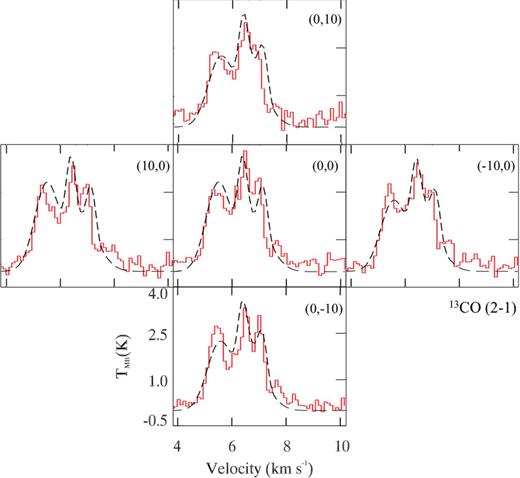
Fig. 8 shows the observed and modelled line emission spectrum for 13CO (J = 2-1). The line profiles are double peaked and asymmetric. The critical density for this transition is three orders of magnitude less than the peak density in B335 so that it probes the optically thick gas far from the centre of the cloud. The asymmetry changes from red-asymmetric (i.e. red > blue) at (20, 0) to blue-asymmetric at (−20, 0).
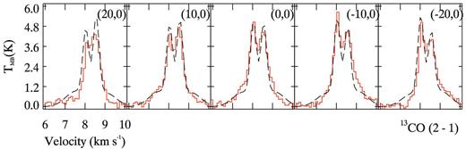
B335: 13CO (J = 2-1) line profiles – observed (solid line) and modelled (dashed line). The offset between cells is 10 arcsec.
Asymmetric, double-peaked line profiles are often taken to be signatures of the presence of infall. However, such an explanation fails to explain the facts that (a) both red and blue asymmetry are present, and (b) asymmetric emission is present at significantly greater offsets (>10 arcsec) than expected for an infall source. A bipolar outflow is therefore a much more likely cause and naturally gives rise to spatially distinct redshifted and blueshifted components. Moreover, outflowing gas has been observed in 12CO (J = 2-1) by Moriarty-Schieven & Snell (1989) extending to 0.36 pc (5 arcmin) either side of IRAS 19347 + 0727. The emission is observed to increase in intensity at the lobe edge. The asymmetry in the line emission profile is essentially caused by the axis of outflow being tilted to the line of sight. Tables 4 and 5 specify the best-fitting parameters for the gas in the outer and inner boundary layers of the outflow.
5.1.2 I04166
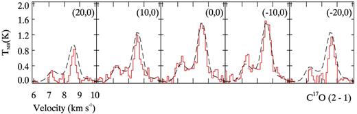
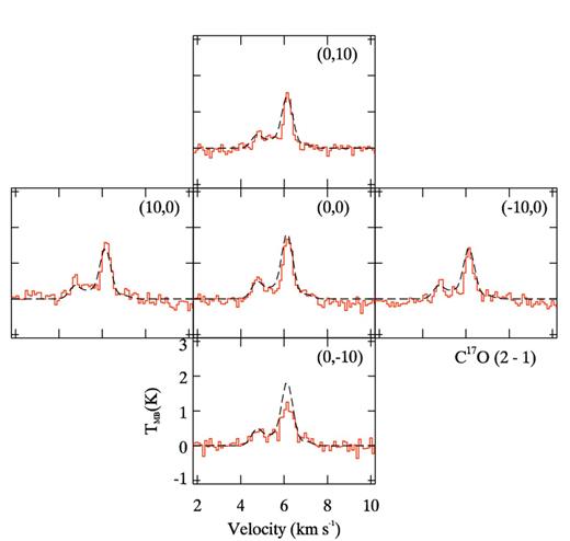
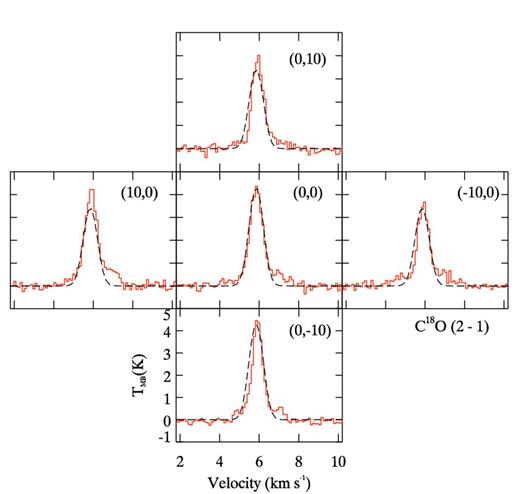
Observations of C17O and C18O (J = 2-1) for I04166 are shown in Figs 9 and 10. The line profiles shown in Fig. 9 clearly show the C17O (J = 2-1) hyperfine line transitions whilst the C18O (J = 2-1) lines shown in Fig. 10 are single-peaked and narrow. Both are characteristic of the quasi-static/slowly infalling gas in the molecular gas envelope. The best-fitting parameters for these profiles (applying to the molecular envelope) are given in Table 3. There is little contribution to the modelled line profile from gas residing in the molecular outflow. We also note that the peak density, as obtained from the 850 μm continuum observations, is consistent with previous estimates derived from N2H+ (J = 1-0) observations (Chen et al. 2007).
I04166: C17O line profiles – observed (solid line) and modelled (dashed line). The offset between cells is 10 arcsec.
I04166: C18O line profiles – observed (solid line) and modelled (dashed line). The offset between cells is 10 arcsec.
The line profiles for 13CO (J = 2-1) are shown in Fig. 11. This shows the standard blue-asymmetric double-peaked line profile suggestive of infalling gas. In addition, there is a component at 5.5 km s−1 which is also seen in the optically thin C18O (J = 2-1) and, to a lesser extent, C17O (J = 2-1) line profiles. It has also been detected in the line profiles of CS (J = 2-1) and H2CO (212–111) (Mardones et al. 1997).
I04166: 13CO (J = 2-1) line profiles – observed (solid line) and modelled (dashed line). The offset between cells is 10 arcsec.
The best-fitting parameters for the infalling envelope component are given in Table 3. The high-velocity gas component at 5.5 km s−1 can be explained by emission originating from the outer boundary layer with the parameters given in Table 4. The wings of the line profile are explained by the high-velocity warm gas in the inner boundary layer that is close to the protostellar jet. The best-fitting parameters for this gas are given in Table 5. Note that the blueshifted emission seen in Fig. 11 is dominant due to the greater amount of absorbing gas on the redshifted side (Tafalla et al. 2004; Santiago-Garcia et al. 2009).
5.1.3 L1527
Figs 12 and 13 show the modelled and observed C17O and C18O (J = 2-1) line profiles, respectively, whilst Fig. 14 shows the H13CO+ (J = 2-1) line. All three profiles are successfully modelled as originating from the molecular gas in the envelope. Specifically, there is no contribution to these line profiles from the gas in the molecular outflows. The best-fitting parameters for these three lines are given in Table 3.
L1527: C17O (J = 2-1) line profiles – observed (solid line) and modelled (dashed line). The offset between cells is 10 arcsec.
L1527: C18O (J = 2-1) line profiles – observed (solid line) and modelled (dashed line). The offset between cells is 10 arcsec.
L1527: H13CO (J = 2-1) line profiles – observed (solid line) and modelled (dashed line). The offset between cells is 10 arcsec.
Fig. 15 shows the modelled and observed line profiles of 13CO (J = 2-1). The core of the line is well fitted by emission from the envelope gas. However, this fails to account for the emission in the wings of the line profile. The best-fitting parameters for the molecular gas in the outflow regions are listed in Tables 4 and 5. The boundary layers of the molecular outflow are fitted with a 13CO:12CO abundance ratio that is significantly enhanced relative to the gas in the envelope.
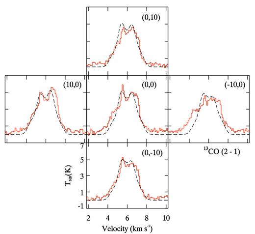
L1527: 13CO (J = 2-1) line profiles – observed (solid line) and modelled (dashed line). The offset between cells is 10 arcsec.
Fig. 16 shows the 12CO (J = 2-1) line emission. This transition traces the large-scale molecular outflow, extending 40 arcsec either side of the IRAS source which is located at the zero offset position. The line profiles are double peaked and asymmetric with the asymmetry changing from blue- to red-asymmetric going from left to right in Fig. 16. Again, this is indicative of the presence of a bipolar outflow. It is consistent with the findings of Myers et al. (1995), who deduced the presence of an outflow with a density >105 cm−3 from observations of H2CO (212–111) and (312–211).
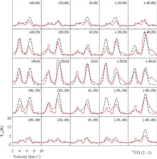
L1527: 12CO (J = 2-1) line profiles – observed (solid line) and modelled (dashed line). The offset between cells is 10 arcsec.
6 DISCUSSION
In this section, the results are discussed in terms of the molecular gas parameters of each of the three components in our model: the molecular gas envelope surrounding the protostellar core and the inner and outer boundary layer regions of the molecular outflow.
6.1 Molecular envelope
The abundances of C18O and C17O are well constrained because the emissions originate from optically thin, quiescent, gas. The situation is somewhat complicated by the action of freeze-out which results in molecular depletion in the inner, denser parts of the core. This process is reversed at the smallest radii, due to heating by the protostar, but on a scale that would be undetectable at JCMT resolution. As described above, we have quantified the level of depletion by comparison of dust continuum and CO line emission maps and find that the maximum depletion factor is ∼10 B335, whilst for I04166 and L1527 it is ∼5. As B335 is the densest and has the largest dust column density of our three sources (see Fig. 3), it is not surprising that it suffers the highest level of gas-phase depletion.
6.2 Outflow abundances in inner and outer boundary layers
The physical parameters of molecular gas in the outflow were constrained by modelling the observed line emission of 12CO (J = 2-1), 13CO (J = 2-1) and HCO+ (J = 3-2) towards each of the sources. Having large abundances, the 13CO (J = 2-1) and 12CO (J = 2-1) transitions can be used to trace the full extent of the outflow. Although HCO+ is abundant in our sources, the (J = 3-2) transition has a very high critical density so that it effectively only traces gas deep inside the molecular envelope close to the base of the outflow.
Tables 4 and 5 show that the molecular abundances tend to be significantly larger in the boundary layers as compared to the cooler envelopes. This is possibly the result of ice mantle evaporation and/or sputtering and may also be due to enhanced gas-phase production in the warmer environments. Thus, Rawlings et al. (2004) proposed a general mechanism for molecular enhancement of HCO+ in a molecular outflow in which carbon atoms, created by the photodissociation of newly desorbed CO gas, are photoionized and react with H2O to form HCO+.
The abundance of H13CO+ was constrained in B335 and L1527. The ratio of 13CO/H13CO+ in each core is ≈2000 though it is slightly higher in L1527. The abundance of 13CO is greatly enhanced in L1527 – by a factor of ∼80 (compared to a factor of ∼2 in B335). This indicates that the fractionation effect discussed above for the formation of 13CO is also feeding through to H13CO+, which is itself formed from 13CO.
Finally, we note again that despite the wide range of line profile appearances, a simple outflow morphology is sufficiently robust for the purpose of analysing the sources. 3D modelling with a code such as mollie enables viewing angle effects to be isolated and reveals the underlying similarities and differences of the sources to be established.
7 SUMMARY AND CONCLUSIONS
We have used a highly simplified physical model of Class 0 protostellar sources, characterized by a spherically symmetric infalling envelope and collimated bipolar outflows – coupled to a 3D radiative transfer code – to model the line emission spectra from molecular gas surrounding three sources. Physical and chemical parameters were initially constrained from observational data and then refined by the modelling and a best-fitting chi-squared analysis.
The simplicity of the model was justified on grounds of structure detectability, due to the limited resolution of single-dish observations. However, using several different gas species in several transitions observed towards three different sources, it was found that this model accurately and self-consistently reproduces the observed spectral line profiles.
The main finding of this study is that, although the three sources we investigate here have dramatically different line profile shapes, we find that once (observationally constrained) infall, depletion and outflow components are introduced, a single morphological model fits all three sources. This verifies the dominance of source morphology in determining line profile shapes. It would be very difficult to fit the data with significantly different physical models, as the detailed structure of the line profiles is largely defined by the physics of the outflow and the envelope. The model and the values of its parameters are essentially defined by empirical constraints. An alternative approach would be to formulate a more detailed theoretical model of the sources and then to attempt to match that with the observations. Such an approach was adopted by Downes & Cabrit (2003) in their hydrodynamic models of jet-driven molecular outflows. From this, they were able to identify a simple intensity–velocity relationship. This was successfully applied, in a modified exponential form, by Lefloch et al. (2012) to fit Herschel-Heterodyne Instrument for the Far Infrared (HIFI) data for five sources. Although this is a different type of modelling from what we have performed – and is applicable to larger scale, higher velocity (>10 km s−1) flows – it should be possible to link consistently the two models.
We find that the principal cause of the source-to-source variations is found to be the difference in the viewing angles; specifically, the angle between the outflow axis and the plane of the sky and not the assumptions about the dynamics of the inflow or outflow. This is evident from the large variations in the line profiles that we have successfully modelled as being primarily due to variation of the viewing angle. No variation of any other parameter or combination of parameters can result in such large differences.
The analysis of the multitransition, spatially resolved line profiles has yielded strong constraints on the chemical and physical parameters of the envelope, outflow and boundary layer of each source. What is remarkable is that the physical parameters for each of the sources, as presented in Tables 3–5, are very similar – the biggest differences between the sources being the abundance ratios of the isotopologues.
We find strong evidence for systemic molecular depletion in all three sources. In addition, we find the following.
The C18O:C17O abundance ratio is approximately the same for each of the sources and is consistent with the value found in interstellar clouds (Schöier et al. 2002).
The abundances of 12CO and 13CO are larger in the bipolar outflow than in the envelope. This is probably a result of thermal evaporation and/or sputtering of the dust ice mantles.
The ratio of the 13CO abundances in the outflow to that in the envelope is ∼3 in B335 and ∼2 in I04166. A much larger value (∼80) is found for L1527. Our previous analysis for L483 yielded a value of ∼32. The ratio for 12CO is ∼2 for both L1527 and L483. These variations perhaps reflect different degrees of dynamical activity in the sources.
As found in L483 (Carolan et al. 2008), there is evidence for 13CO being preferentially enhanced over 12CO in L1527, probably due to chemical fractionation effects.
These studies clearly show the importance of the adoption of realistic morphological/dynamical models of infall/outflow sources, coupled with full 3D radiative transfer codes in the analysis of star-forming regions. This approach will be essential in the analysis of Atacama Large Millimeter Array (ALMA) data and in focusing on the small-scale structure of the outflows. On these small scales, many of our simplifying assumptions (such as that of isothermality) will no longer be applicable. In these situations, the model will need to be modified to include a detailed thermal structure and the effects of more complex morphologies and substructure in the outflows.
We thank Eric Keto, Robin Garrod and David Williams for useful discussions and assistance with the observational and modelling work. We also thank an anonymous referee for constructive comments. The James Clerk Maxwell Telescope is operated by the Joint Astronomy Centre on behalf of the Science and Technology Facilities Council of the United Kingdom, the Netherlands Organisation for Scientific Research and the National Research Council of Canada. MPR acknowledges the support from a Science Foundation Ireland Research Frontiers Programme grant (06RFP/PHY051) and from the COST Action CM0805 ‘The Chemical Cosmos’.
REFERENCES
APPENDIX A: ESTIMATING N(H2) FROM C18O OBSERVATIONS
In our models, an excitation temperature of 10 K is assumed (consistent with the dust temperature) yielding a C18O rotational partition function of ∼7.94. μ is the dipole moment which for C18O is 0.110 79 debye (Pickett et al. 1998). A conversion factor of 2.07 × 10⁶ is used to convert the C18O column density into the H2 column density (Lacy et al. 1994; Wilson & Rood 1994; Ladd, Fuller & Deane 1998).
