Catastrophic evaporation of rocky planets

Abstract

1 INTRODUCTION

Atmospheric escape shapes the faces of planets. Mechanisms for mass-loss vary across the Solar system. Planets lacking magnetic fields can be stripped of their atmospheres by the solar wind: the atmospheres of both Mercury and Mars are continuously eroded and refreshed by solar wind ions (Potter & Morgan 1990, 1997; Lammer & Bauer 1997; Bida, Killen & Morgan 2000; Jakosky & Phillips 2001; Killen et al. 2004). Venus demonstrates the extreme sensitivity of atmospheres to stellar insolation. Although its distance to the Sun is only 30 per cent less than that of the Earth, Venus has lost its water to hydrodynamic escape powered by solar radiation (Kasting & Pollack 1983; Zahnle & Kasting 1986). Impacts with comets and asteroids can also purge planets of their atmospheres, as is thought to have happened to some extent on Mars (Melosh & Vickery 1989; Jakosky & Phillips 2001) and some giant planet satellites (Zahnle et al. 1992). An introductory overview of atmospheric escape in the Solar system is given by Catling & Zahnle (2009).

Smaller bodies lose their atmospheres more readily because of their lower surface gravities. Bodies closer to their host star also lose more mass because they are heated more strongly. Extrasolar planets on close-in orbits are expected to have highly processed atmospheres. In extreme cases, stellar irradiation might even evaporate planets in their entirety – comets certainly fall in this category.

Hot Jupiters are the best studied case for atmospheric erosion in extrasolar planets (for theoretical models, see Yelle 2004, 2006; Tian et al. 2005; García Muñoz 2007; Holmström et al. 2008; Murray-Clay, Chiang & Murray 2009; Ekenbäck et al. 2010; Tremblin & Chiang 2013). For these gas giants, mass-loss is driven by stellar ultraviolet (UV) radiation which photoionizes hydrogen and imparts enough energy per proton to overcome the planet's large escape velocity (∼60 km s⁻¹). Mass-loss for hot Jupiters typically occurs at a rate of |$\dot{M} \sim 10^{10}$|–10¹¹ g s⁻¹ so that ∼1 per cent of the planet mass is lost over its lifetime (Yelle 2006; García Muñoz 2007; Murray-Clay et al. 2009). Although this erosion hardly affects a hot Jupiter's internal structure, the outflow is observable. Winds escaping from hot Jupiters have been spectroscopically detected by the Hubble Space Telescope. During hot Jupiter transits, several absorption lines (H i, O i, C ii, Mg ii and Si iii) deepen by ∼2–10 per cent (Vidal-Madjar et al. 2003, 2004, 2008; Ben-Jaffel 2007, 2008; Fossati et al. 2010; Lecavelier Des Etangs et al. 2010; Linsky et al. 2010; Lecavelier des Etangs et al. 2012).

Because of their lower escape velocities, lower mass super-Earths should have their atmospheres more significantly sculpted by evaporation. Lopez, Fortney & Miller (2012) found that hydrogen-dominated atmospheres of close-in super-Earths could be stripped entirely by UV photoevaporation (e.g. Kepler-11b).

At even lower masses and stellocentric distances, planets might evaporate altogether. When dayside temperatures surpass ∼2000 K, rocks, particularly silicates and iron (and to a lesser extent, Ti, Al and Ca), begin to vaporize. If the planet mass is low enough, thermal velocities of the high-metallicity vapour could exceed escape velocities. Under these circumstances, mass-loss is not limited by stellar UV photons, but is powered by the incident bolometric flux.

1.1 KIC 12557548b: a catastrophically evaporating planet

In fact, the Kepler spacecraft may have enabled the discovery of an evaporating, close-in rocky planet near the end of its life. As reported by Rappaport et al. (2012), the K star KIC 12557548 dims every 15.7 h by a fractional amount f that varies erratically from a maximum of f ≈ 1.3 per cent to a minimum of f ≲ 0.2 per cent. These occultations are thought to arise from dust embedded in the time-variable outflow emitted by an evaporating rocky planet – hereafter KIC 1255b. Because Kepler observes in the broad-band optical, the obscuring material cannot be gas which absorbs only in narrow lines; it must take the form of dust which absorbs and scatters efficiently in the continuum. As we will estimate shortly, the amount of dust lost by the planet is prodigious.

From the ∼2000 K surface of the planet is launched a thermal (‘Parker-type’) wind out of which dust condenses as the gas expands and cools. The composition of the high-metallicity wind reflects the composition of the evaporating rocky planet (see e.g. Schaefer & Fegley 2009): the wind may consist of Mg, SiO, O and O₂ – and Fe if it has evaporated down to its iron core. Stellar gravity, together with Coriolis and radiation-pressure forces, then shapes the dusty outflow into a comet-like tail. The peculiar shape of the transit light curve of KIC 1255b supports the interpretation that the occultations are caused by a dusty tail. First, the light curve evinces a flux excess just before ingress, which could be caused by the forward scattering of starlight towards the observer. Secondly, the flux changes more gradually during egress than during ingress, as expected for a trailing tail. Both features of the light curve and their explanations were elucidated by Rappaport et al. (2012), and further quantified by Brogi et al. (2012), who presented a phenomenological light-scattering model of a dusty tail.¹

Spectra of KIC 12557548 taken using the Keck telescope reveal no radial velocity variations down to a limiting accuracy of ∼100 m s⁻¹ (Howard & Marcy, personal communication). A deep Keck image also does not reveal any background blended stars. These null results are consistent with the interpretation that KIC 1255b is a small, catastrophically evaporating planet.

Rappaport et al. (2012) claimed that the present-day mass of KIC 1255b is ∼0.1 M_⊕. They estimated, to order of magnitude, the maximum planet mass that could reproduce the observed mass-loss rate given by equation (5). Here we revisit the issue of planet mass – and the evaporative lifetime it implies – with a first-principles solution of the hydrodynamic equations for a planetary wind, including an explicit treatment of dust–gas thermodynamics. We will obtain not only improved estimates of the present-day mass, but also full dynamical histories of KIC 1255b.

1.2 Plan of this paper

We develop a radiative hydrodynamic wind model to study the mass-loss of close-in rocky planets with dayside temperatures high enough to vaporize rock. Although our central application will be to understand KIC 1255b – both today and in the past – the model is general and can easily be modified for parameters of other rocky planets.

The paper is structured as follows. In Section 2, we present the model that computes |$\dot{M}$| as a function of planet mass M. We give results in Section 3, including estimates for the maximum present-day mass and the maximum formation mass of KIC 1255b. A wide-ranging discussion of the implications of our results – including, e.g., an explanation of why mass-loss in this context does not obey the often-used energy-limited mass-loss formula (cf. Lopez et al. 2012), as well as the prospects of detecting close-in Mercuries and stripped iron cores – is given in Section 4. Our findings are summarized in Section 5.

2 THE MODEL

We construct a 1D model for the thermally driven atmospheric mass-loss from a close-in rocky planet, assuming that it occurs in the form of a transonic Parker wind. The atmosphere of the planet consists of a high-metallicity gas created by the sublimation of silicates (and possibly iron, as we discuss in Section 4.7) from the planetary surface. We focus on the flow that streams radially towards the star from the substellar point on the planet. The substellar ray is of special interest because the mass flux it carries will be maximal insofar as the substellar point has the highest temperature – and thus the highest rate of rock sublimation – and insofar as stellar gravity will act most strongly to accelerate gas away from the planet.

As the high-metallicity gas flows away from the surface of the planet, it will expand and cool, triggering the condensation of dust grains. Dust grains can affect the outflow in several ways: (a) latent heat released during the condensation of grains will heat the gas; (b) continuously heated by starlight, grains will transfer their energy to the gas via gas–grain collisions; and (c) absorption/scattering of starlight by grains will reduce the stellar flux reaching the planet, reducing the surface temperature and sublimation rate. In this work, we do not account for the microphysics of grain condensation, as cloud formation is difficult to calculate from first principles (see e.g. the series of five papers beginning with Helling et al. 2001; see also Helling et al. 2008a; Helling, Woitke & Thi 2008b). Instead, we treat the dust-to-gas mass fraction x_dust as a free function and explore how our results depend on this function. In our one-fluid model, dust grains are perfectly entrained in the gas flow, an assumption we test a posteriori (Section 4.2).

We begin in Section 2.1 by evaluating thermodynamic variables at the surface of the planet – the inner boundary of our model. In Section 2.2, we introduce the 1D equations of mass, momentum and energy conservation. In Section 2.3, we explain the relaxation method employed to solve the conservation laws.

2.1 Base conditions of the atmosphere

Figure 1.

Open in new tabDownload slide

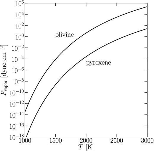
Equilibrium vapour pressures of pyroxene and olivine versus temperature, obtained from equation (7).

2.2 Equations solved

As dust condenses from gas and x_dust rises, the gas density ρ must fall by mass conservation. For simplicity, we neglect the dependence of ρ on x_dust and so restrict our analysis to x_dust, max ≪ 1; in practice, the maximum value of x_dust, max that we consider is 10^−0.5 ≈ 0.32.

2.3 Relaxation code

The structure of the wind is found by the simultaneous solution of equations (10), (11), (12) and (16) with the appropriate boundary conditions. This system constitutes a two-point boundary value problem, as the boundary conditions for ρ and T are defined at the base of the flow, while those for v and τ are defined at the sonic point.

Although generally more complicated, relaxation codes are preferred over shooting methods when solving for the transonic Parker wind. This is because for each transonic solution there are an infinite number of ‘breeze solutions’ where the bulk speed of the wind never reaches supersonic velocities. It is easier to begin with an approximate solution that already crosses the sonic point and to then refine this solution, than to exhaustively shoot in multidimensional space for the sonic point. Murray-Clay et al. (2009) used a relaxation code to find the transonic wind from a hot Jupiter. Here we follow their methodology; we develop a relaxation code based on section 17.3 of Press et al. (1992).

2.3.1 Finite-difference equations

2.3.2 Boundary conditions

2.3.3 Method of solution

The relaxation method determines the solution by starting with an appropriate guess and iteratively improving it. We use the multidimensional Newton's method as our iteration scheme, which requires us to evaluate partial derivatives of all E_{i, j} with respect to all 4N dependent variables (ρ_j, T_j, v_j, τ_j). We evaluate partial derivatives numerically, by introducing changes of the order of 10⁻⁸ in dependent variables and computing the appropriate finite differences. Newton's method produces a 4N × 4N matrix, which we invert using the numpy library in python. At each iteration, we numerically solve equation (26) for r_s and re-map all N grid points between R and r_s. We iterate until variables change by less than one part in 10¹⁰.

We found our iteration scheme to be rather fragile. The code only converges if initial guesses are already close to the solution. For this reason, we started with a simplified version of the problem with a known analytic solution as the initial guess. We then gradually added the missing physics to the code, obtaining a solution with each new physics input until the full problem was solved. Specifically, we began by solving the isothermal Parker wind problem (e.g. Lamers & Cassinelli 1999). We enforced the isothermal condition by declaring γ to be unity, so that our energy equation reads dT/dr = 0 (see equation 21). Additionally, we set M_* and x_dust to zero to remove the effects of tidal gravity and dust. We then slowly increased each of the parameters M_*, γ and x_dust (in that order) to their nominal values. Any subsequent parameter change (e.g. M) was also performed in small increments.

3 RESULTS

We begin in Section 3.1 with an isothermal gas model. The isothermal model serves both as a limiting case and as a starting point for developing the full solution which includes a realistic treatment of the energy equation. We provide results for our full model in Section 3.2. In the full solution we focus on three possible planet masses M = 0.01, 0.03 and 0.07 M_⊕, finding that M ≈ 0.01 M_⊕ yields a maximum|$\dot{M}$| that is compatible with the observationally inferred |$\dot{M}_{\rm {1255b}}$|⁠. We conclude that in the context of our energy equation, the present-day mass of KIC 1255b is at most ∼0.02 M_⊕ (since smaller mass planets can generate still higher |$\dot{M}$| that are also compatible with |$\dot{M}_{\rm {1255b}}$|⁠). In Section 3.3, we integrate back in time to compute the maximum formation mass of KIC 1255b.

3.1 Isothermal solution

We begin by solving a steady, dust-free, isothermal wind described by equations (10) and (11) with M_* set equal to zero. Although this is a highly idealized problem, its solution provides us with a starting point (i.e. an initial model) from which we are able to solve more complicated problems (see Section 2.3.3). Our code accepts the standard isothermal wind solution (e.g. chapter 3 of Lamers & Cassinelli 1999) as an initial guess, with minimal relaxation.

Figure 2.

Open in new tabDownload slide

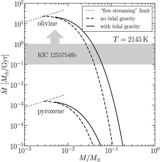
Evaporative mass-loss rates |$\dot{M}$| versus planet mass M for isothermal dust-free winds. The solid lines are for models that include stellar tidal gravity, while the dashed curves are for models that do not. As the planet mass is reduced, all solutions converge towards the free-streaming limit where |$\dot{M}$| is not influenced by gravity but instead scales with the surface area of the planet (equation 28). As inferred from observations, possible present-day mass-loss rates |$\dot{M}_{\rm {1255b}}$| for KIC 1255b are marked in grey. Technically we have only a lower limit on |$\dot{M}_{\rm {1255b}}$| of 0.1 M_⊕ Gyr⁻¹; for purposes of discussion throughout this paper, we adopt 0.1–1 M_⊕ Gyr⁻¹ as our fiducial range (see the discussion surrounding equation 5). Clearly KIC 1255b cannot be a pure pyroxene planet. Subsequent figures will refer to planets with pure olivine surfaces (except in Section 4.7 where we consider iron).

3.2 Full solution

We relax the isothermal condition in our code by slowly increasing γ from 1 to 1.3. With this parameter change, we are solving the full energy equation (equation 12). Grains are gradually added by modifying x_dust, amp and x_dust, max, necessitating the calculation of optical depth (equation 16).

In Fig. 3, we show the solution for which |$\dot{M}$| was maximized (over the space of possible values of x_dust) for M = 0.03 M_⊕, or about half the mass of Mercury. Recall from Section 3.1 that when the wind was assumed to be isothermal, a planet of this mass was able to reproduce the inferred mass-loss rate of KIC 1255b. Now, with our treatment of the full energy equation and the inclusion of dust, |$\max \dot{M}$| plummets by a factor of 40. Relative to the isothermal solution, the reduction in mass-loss rate in the full model is mainly caused by the gas temperature dropping from 2095 K at the planet surface to below 500 K at the sonic point, and the consequent reduction in gas pressure. The temperature drops because gas expands in the wind and does PdV work. Gas heating by dust–gas collisions or grain formation could, in principle, offset some of the temperature reduction, but having too many grains also obscures the surface from incident starlight, decreasing T_surface and ρ_vapour (the latter quantity depends exponentially on the former). The particular dust-to-gas profile x_dust that is used in Fig. 3 is such that the ability of dust to heat gas is balanced against the attenuation of stellar flux by dust, so that |$\dot{M}$| is maximized (for this M).

Figure 3.

Open in new tabDownload slide

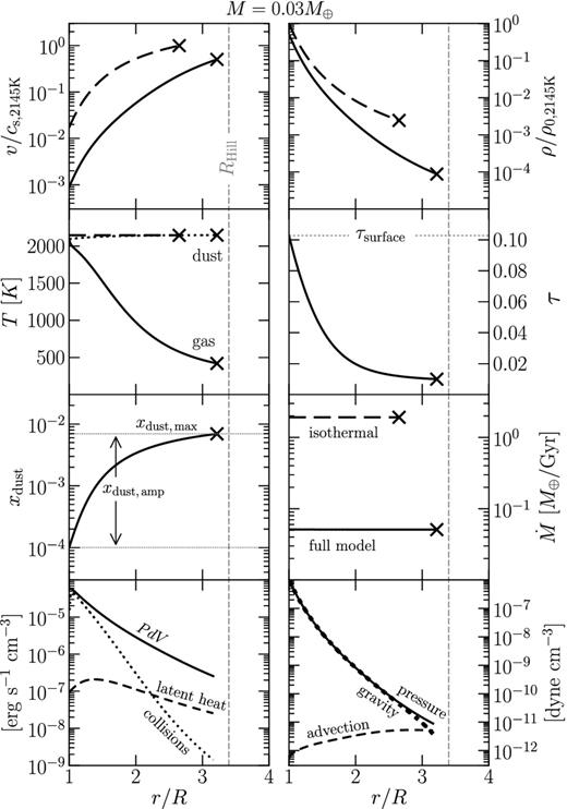
Radial dependence of wind properties in the full solution for a planet of mass M = 0.03 M_⊕. Parameters of the x_dust function are chosen to maximize |$\dot{M}$|⁠. In the upper six panels, the full solution is shown by solid curves, while the dust-free isothermal solution is marked by dashed curves. Values for v have been normalized to the sound speed at T = 2145 K, and values for ρ have been normalized to the density ρ_{0, 2145K} = μP_vapour/(kT) evaluated also at T = 2145 K. The ×-symbol marks the location of the sonic point (the outer boundary of our solution), which occurs close to the Hill radius R_Hill (marked by a vertical line). The two lower panels show the contributions of the individual terms in the energy and momentum equations (left- and right-hand panels, respectively).

Note that the flow at the base begins with velocities of ∼10⁻³ the sound speed. At these subsonic velocities, the atmosphere is practically in hydrostatic equilibrium, with gas pressure and gravity nearly balancing. Only when velocities are nearly sonic does advection become a significant term in the momentum equation (bottom-right panel of Fig. 3). Flow speeds are still high enough at the base of the atmosphere to lift dust grains against gravity for all but the highest planet masses considered (Section 4.2; gas speeds as low as ∼1 m s⁻¹ in an ∼ 1 μbar atmosphere can enable micron-sized grains to escape sub-Mercury-sized planets, as can be verified by equation (30); furthermore, the condition that grains not slip relative to gas is conveniently independent of gas velocity in the Epstein free molecular drag regime, as can be seen in equation (29). Our flows are entirely in the Epstein drag regime, as explained below equation (29).

In Fig. 4, we show how |$\dot{M}$| and τ_surface vary with the function x_dust. As just discussed, |$\max \dot{M}$| is reached for a specific choice of parameters which balance gas heating by dust and surface obscuration by dust. (We emphasize, here and elsewhere, that we have not identified a physical reason why actual systems like KIC 1255b should have mass-loss rates |$\dot{M}$| that equal their theoretically allowed maximum values.) Apart from the region near the peak in |$\dot{M}$|⁠, contours of constant τ_surface are roughly parallel to contours of constant |$\dot{M}$|⁠, suggesting that the value of τ_surface is more important for determining |$\dot{M}$| than the specific functional form of x_dust. This finding increases the confidence we have in the robustness of our solution.

Figure 4.

Open in new tabDownload slide

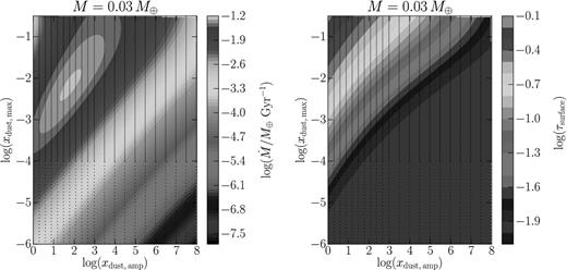
Left-hand panel: dependence of |$\dot{M}$| on dust abundance for a planet of mass M = 0.03 M_⊕. The dust abundance parameters x_dust, max and x_dust, amp are defined in equation (19); see also Fig. 3. Both parameters are varied independently to find the maximum |$\dot{M}$|⁠, which occurs at log(x_dust, amp, x_dust, max) ∼ (1.7, −2.2). The full model corresponding to this maximum |$\dot{M}$| is detailed in Fig. 3. Each black dot corresponds to a full model solution. Colour contours for |$\dot{M}$| are interpolated using a cubic polynomial. Right-hand panel: optical depth τ_surface between the star and the planetary surface as a function of dust abundance for a planet of mass M = 0.03 M_⊕. Apart from the region near the peak in |$\dot{M}$|⁠, contours of constant τ_surface are roughly parallel to contours of constant |$\dot{M}$|⁠, suggesting that the value of τ_surface is more important for determining |$\dot{M}$| than the specific functional form of x_dust.

It is clear from Figs 3 and 4 that a planet of mass M = 0.03 M_⊕ can only emit winds for which |$\max \dot{M} < \min \dot{M}_{\rm {1255b}} \sim 0.1\, {\rm M}_{\rm {{\oplus }}}$| Gyr⁻¹ (at least within the context of our energy equation). In Fig. 5, we show results for M = 0.01 M_⊕, for which |$\max \dot{M} > \min \dot{M}_{\rm {1255b}}$|⁠. For this M, the mass-loss rate |$\dot{M}$| is maximized when the planet surface is essentially unobscured by dust. At our arbitrarily chosen value for x_dust ∼ 3 × 10⁻⁷, the wind is not significantly heated by dust and expands practically adiabatically. The maximum |$\dot{M}$| is reached for an essentially dust-free solution because the wind is blowing at too high a speed for dust–gas collisions to be important. That is, the time-scale over which gas travels from the planet's surface to the sonic point is shorter than the time it takes a gas particle to collide with a dust grain: gas is thermally decoupled from dust. Were we to increase x_dust to make dust–gas heating important, the flow would become optically thick and the wind would shut down. If the model shown in Fig. 5 does represent KIC 1255b, then the dust grains that occult the star must condense outside the sonic point, beyond the Hill sphere.

Figure 5.

Open in new tabDownload slide

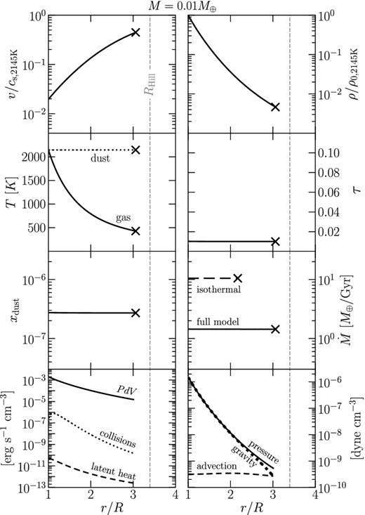
Same as Fig. 3, but for a planet of mass M = 0.01M_⊕. For this planet mass, |$\dot{M}$| is maximized when essentially no dust is present (i.e. the atmosphere is essentially transparent) as gas moves too quickly for dust–gas collisions to heat the gas. As such, all heating terms are negligible and the gas expands adiabatically.

Fig. 6 shows the solution for M = 0.07 M_⊕. In this case, |$\dot{M}$| is maximized when enough dust is present to heat the gas significantly above the adiabat. At this comparatively large planet mass, initial wind speeds are low enough that a gas particle collides many times with dust over the gas travel time, so that dust–gas collisions heat the gas effectively near the surface of the planet. Further downwind, near the sonic point, latent heating overtakes PdV cooling and actually increases the temperature of the gas with increasing altitude. The wind is much more sensitive to heating near the base of the flow than near the sonic point: if we omit latent heating from our model – so that gas cools to ∼500 K at the sonic point – then |$\dot{M}$| is reduced by only a factor of 2. In comparison, |$\dot{M}$| drops by several orders of magnitude if dust–gas collisions are omitted.

Figure 6.

Open in new tabDownload slide

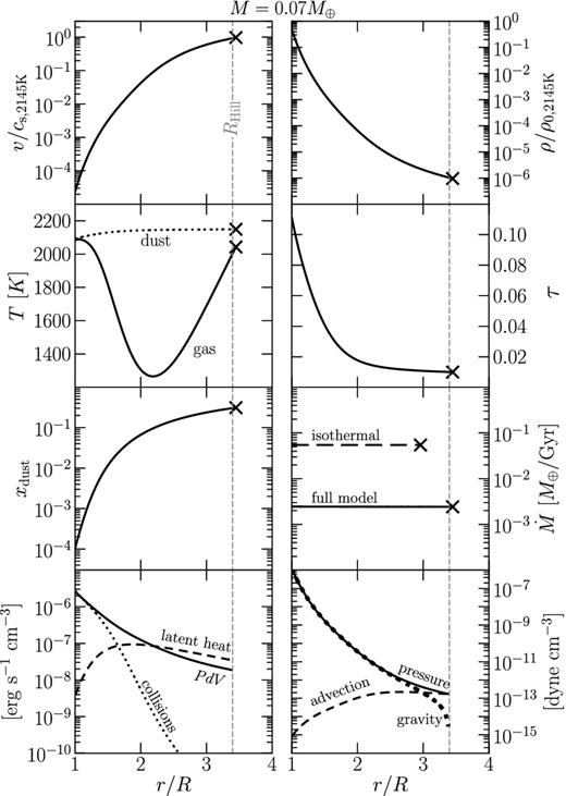
Same as Fig. 3, but for a planet of mass M = 0.07M_⊕. For this mass, |$\dot{M}$| is maximized for the dustiest flows considered in this paper. The outflow is launched at such low velocities that collisional dust–gas heating is important. Near the sonic point, latent heating overtakes PdV cooling and the temperature of the gas rises.

The dependence of |$\dot{M}$| on x_dust in both the ‘dust-free low-mass’ and the ‘dusty high-mass’ limits is illustrated in Fig. 7. In the low-mass limit, |$\dot{M} = \max \dot{M}$| when no dust is present. In this regime, gas moves too quickly for heating by dust to be significant; dust influences the flow only by attenuating starlight, and as long as τ_surface ≪ 1, dust hardly affects |$\dot{M}$|⁠. By contrast, in the high-mass limit, |$\dot{M} = \max \dot{M}$| for the dustiest flows we consider (i.e. the highest values of x_dust, max). In this regime, |$\dot{M}$| is very sensitive to dust abundance, with values spanning six orders of magnitude over the explored parameter space.

Figure 7.

Open in new tabDownload slide

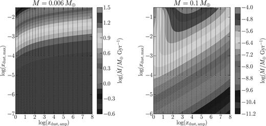
Left-hand panel: same as the left-hand panel of Fig. 4, but for a planet of mass M = 0.006 M_⊕. In this low-mass limit, |$\dot{M}$| is maximized when no dust is present (i.e. when the atmosphere is transparent) because gas is moving too quickly for heating by dust to be significant. Right-hand panel: same as the left-hand panel, but for a planet of mass M = 0.1M_⊕. In this high-mass limit, |$\dot{M}$| is maximized for the dustiest flows we consider (i.e. the highest values of x_{dust, max}) because flow speeds near the surface are slow enough for dust–gas energy exchange to be significant.

In Fig. 8, we show mass-loss rates as a function of planet mass for the full model. We emphasize that these are maximum mass-loss rates, found by varying x_dust. At low planet masses, |$\max \dot{M}$| for the full model converges with |$\dot{M}$| for the isothermal model because both approach the free-streaming limit, where gravity becomes irrelevant and |$\dot{M}$| is set entirely by conditions at the surface of the planet (equation 28). To reach |$\dot{M}_{\rm {1255b}} > 0.1\, {\rm M}_{\rm {{\oplus }}}$| Gyr⁻¹, the present-day mass of KIC 1255b must be ≲ 0.02 M_⊕, or less than about twice a lunar mass.

Figure 8.

Open in new tabDownload slide

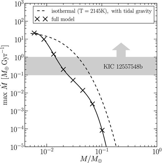
Maximum mass-loss rates |$\dot{M}$| versus planet mass M for the full model. At each ×-marked mass, max |$\dot{M}$| was found by varying x_dust as described, e.g. in Fig. 4. The solid curve denotes a cubic spline interpolation. Mass-loss rates for the full model are generally lower than for the isothermal model (dashed curve) because the dust–gas heating terms we have included in our full model turn out to be inefficient. At low planet masses, the isothermal and full models converge because both approach the free-streaming limit, where gravity becomes irrelevant and |$\dot{M}$| is set entirely by conditions at the surface (i.e. surface area, equilibrium vapour pressure and sound speed; equation 28). According to the full model, the present-day mass of KIC 1255b is ≲ 0.02 M_⊕, or less than twice the mass of the Moon; for such masses, |$\max \dot{M} > \min \dot{M}_{1255b} \sim 0.1 \,{\rm M}_{\rm {{\oplus }}}$| Gyr⁻¹.

We have verified a posteriori for the models shown in Figs 3, 5 and 6 that the sonic point is attained at an altitude where the collisional mean free path of gas molecules is smaller than r_s, so that the hydrodynamic approximation embodied in equations (10)–(12) is valid. In other words, the exobase lies outside the sonic point in these |$\dot{M}=\max \dot{M}$| models. The margin of safety is largest for the lowest mass models.

3.3 Mass-loss histories

We calculate mass-loss histories M(t) by time-integrating our solution, shown in Fig. 8, for |$\max \dot{M}(M)$|⁠. Before we integrate, however, we introduce 0 < f_duty < 1 to account for the duty cycle of the wind: we define |$f_{\rm {duty}} \cdot \max \dot{M}$| as the time-averaged mass-loss rate. We estimate that f_duty ∼ 0.5 based on the statistics of transit depths compiled by Brogi et al. (2012, see their fig. 2). We time-integrate |$f_{\rm {duty}} \cdot \max \dot{M}$| to obtain the M(t) curves shown in Fig. 9. (This factor of 2 correction for the duty cycle should not obscure the fact that the actual mass-loss rate, time-averaged or otherwise, could still be much lower than the theoretically allowed |$\max \dot{M}$|⁠, a possibility we return to throughout this paper.)

Figure 9.

Open in new tabDownload slide

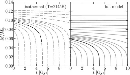
Mass-loss histories M(t) obtained by time-integrating |$f_{\rm {duty}} \cdot \max \dot{M}(M)$| with f_duty = 0.5 for the isothermal and full models. We highlight the case of a planet with a 5 Gyr lifetime. For the full model (right-hand panel), this corresponds to an initial mass of ∼0.06 M_⊕, slightly larger than the mass of Mercury. Such a planet could have formed in situ and slowly eroded over several Gyr until reaching ∼0.03 M_⊕, whereupon the planet evaporates completely in a few hundred Myr. By contrast, planets with formation masses ≳ 0.07 M_⊕ survive (in the full model) for tens of Gyr without significant mass-loss.

We highlight the case of a planet with a lifetime of t_life = 5 Gyr. Under our full (non-isothermal) model (right-hand panel of Fig. 9), such a planet has a mass at formation of 0.06 M_⊕ and gradually erodes over several Gyr until it reaches M ∼ 0.03 M_⊕ – whereupon the remaining mass is lost catastrophically over a short time (just how short is estimated for the specific case of KIC 1255b below). Contrast this example with planets having initial masses ≳0.07 M_⊕ – these have such low |$\dot{M}$| that they barely lose any mass over Gyr time-scales.

For comparison, we also present mass-loss histories using a dust-free isothermal model with stellar tidal gravity (left-hand panel of Fig. 9). Compared to our non-isothermal solutions – for which gas temperatures fall immediately as the wind lifts off the planet surface – the isothermal solution corresponds to a flow which stays relatively pressurized and which therefore enjoys the largest |$\dot{M}$| for a given M. The isothermal wind thus represents an end-member case. However, the mass-loss histories under the isothermal approximation do not differ qualitatively from those using the full energy equation. For isothermal winds, the dividing mass between planet survival and destruction within 10 Gyr is about 0.11 M_⊕, only ∼40 per cent larger than the value cited above for our non-isothermal solutions.

3.4 Possible mass-loss histories for KIC 1255b

Figs 8 and 9 can be used to sketch possible mass-loss histories for KIC 1255b. For our first scenario, we employ the full model that solves the full energy equation. Today, to satisfy the observational constraint that |$\dot{M}_{\rm {1255b}} > 0.1 \, {\rm M}_{\rm {{\oplus }}}\,{\rm Gyr^{-1}}$| (see the derivation of our equation 5), the planet must have a present-day mass of at mostM ≈ 0.02 M_⊕, or roughly twice the mass of the Moon (Fig. 8). Such a low mass implies that currently KIC 1255b is in a ‘catastrophic evaporation’ phase (vertical straight lines in Fig. 9). Depending on the age of the planet (i.e. the age of the star: 1–10 Gyr), KIC 1255b originally had a mass of at most 0.04–0.07 M_⊕: two to four times its maximum current mass, or about the mass of Mercury. Starting from today, the time the planet has before it disintegrates completely is of the order of |$t_{\rm {evap}} \sim M/(f_{\rm {duty}} \cdot \max \dot{M})$|⁠, which is as long as 400 (40) Myr for M = 0.02 M_⊕, f_duty = 0.5 and |$\max \dot{M} = 0.1$| (1) M_⊕ Gyr⁻¹.

If our energy equation were somehow in error and the wind better described as isothermal, then the numbers cited above would change somewhat. The present-day mass of KIC 1255b would be at most M ∼ 0.07 M_⊕; the maximum formation mass would be between 0.08 and 0.11 M_⊕; and the evaporation time-scale starting from today could be as long as t_evap ∼ 400 Myr if the present-day mass M ∼ 0.07 M_⊕.

As we have stressed throughout, a critical assumption we have made is that the time-averaged mass-loss rate is |$f_{\rm {duty}} \cdot \max \dot{M}$| with f_duty as high as 0.5. We have not identified a physical reason why the actual mass-loss rate should be comparable to the theoretically allowed |$\max \dot{M}$| for a given M. If our assumption were in error and actual mass-loss rates |$\dot{M} \ll \max \dot{M}$|⁠, then the present-day mass of KIC 1255b, the corresponding evaporation time and the formation mass of KIC 1255 would all decrease from the upper bounds cited above.

The degeneracy of possible masses and evaporative histories outlined in this section could be broken with observational searches for the progenitors of KIC 1255b-like objects (Section 4.6).

4 DISCUSSION

We discuss how mass-loss is not ‘energy limited’ in Section 4.1; how gas entrains dust in Section 4.2; how the evaporative wind can be time variable in Section 4.3; the effects of winds on orbital evolution in Section 4.4; the interaction of the planetary wind with the stellar wind in Section 4.5; the occurrence rate of quiescent progenitors of catastrophically evaporating planets in Section 4.6; the possibility that evaporating planets can be naked iron cores in Section 4.7; and the ability of dust to condense out of the wind in Section 4.8.

4.1 Mass-loss is not energy limited

Atmospheric mass-loss rates are commonly assumed to be ‘UV-energy limited’: it is assumed that a fixed, order-unity fraction ϵ of the incident UV flux F_UV does PdV work and lifts material out of the planet's gravitational well. Under the energy-limited assumption, the mass-loss rate is |$\dot{M} \sim \epsilon \pi R^2 F_{\rm {UV}}/(GM/R)$|⁠. The validity of this formula has been tested by Watson, Donahue & Walker (1981) for terrestrial atmospheres and by Murray-Clay et al. (2009) for hot Jupiters.

The energy-limited formula does not apply at all to the evaporating rocky planets considered in this paper. The stellar UV flux is not essential for low-mass planets because their escape velocities are so small that energy deposition by photoionization is not necessary for driving a wind. Even optical photons – essentially the stellar bolometric spectrum – can vaporize close-in planets. Merely replacing F_UV with F_bolometric in the energy-limited formula would still be misleading, however, because most of the incident energy is radiated away and does no mechanical work. More to the point, ϵ is not constant; as discussed in Section 3.2, the energetics of the flow changes qualitatively with planet mass. If we were to insist on using the energy-limited formula, we would find ϵ ∼ 10⁻⁸ for M ∼ 0.1 M_⊕ and ϵ ∼ 10⁻⁴ for M ∼ 0.01 M_⊕ (see Fig. 8).

4.2 Dust–gas dynamics

We find using our full model (for |$\dot{M} = \max \dot{M}$|⁠) that t_stop/t_adv < 1 everywhere for M < 0.03 M_⊕, confirming our assumption that micron-sized (and smaller) grains are well entrained in the winds emanating from such low-mass planets. When M = 0.03 M_⊕, t_stop < t_adv close to the planet's surface, but as gas nears the sonic point, t_stop becomes comparable to t_adv. For M > 0.03 M_⊕, the one-fluid approximation breaks down near the sonic point. For such large planet masses, future models should account for gas–grain relative motion – in addition to other effects that become increasingly important near the sonic point/Hill sphere boundary (e.g. Coriolis forces and stellar radiation pressure). Note that the one-fluid approximation should be valid for the present-day dynamics of KIC 1255b, since according to the full model its current mass is at most M ≈ 0.02 < 0.03 M_⊕.

For M ≈ 0.03 M_⊕ and our adopted grain size s = 1 μm, the forces in equation (30) are comparable near the sonic point when v_rel ∼ c_s (i.e. when grains are barely lifted by drag). For M > 0.03 M_⊕, micron-sized and larger grains will not be dragged past the sonic point according to (30) – thus our assumption that they do fails for such high-mass planets and will need to be rectified in future models. Smaller, sub-micron-sized grains can, however, be lifted outwards. Moreover, sub-micron-sized grains may heat the gas more effectively because they have greater geometric surface area for dust–gas collisions (at fixed x_dust) and because their temperatures exceed those of blackbodies (their efficiencies for emission at infrared wavelengths are much less than their absorption efficiencies at optical wavelengths). The superior momentum and thermal coupling enjoyed by grains having sizes s ≪ 1 μm, plus their relative transparency at optical wavelengths – which helps them avoid shadowing the planet surface from stellar radiation – motivate their inclusion in the next generation of models.

Our model could be improved still further by self-consistently accounting for how the gas density ρ must decrease as dust grains condense out of gas. Moreover, the restriction that x_dust < 1 could be lifted.

4.3 Time variability

Occultations of KIC 12557548 vary in depth from a maximum of 1.3 per cent to a minimum of ≲0.2 per cent on orbital time-scales. Rappaport et al. (2012) discussed qualitatively the possibility that such transit depth variations arise from a limit cycle that alternates between high-|$\dot{M}$| and low-|$\dot{M}$| phases. A high-|$\dot{M}$| phase that produces a deep eclipse would also shadow the planet surface from starlight. The resultant cooling would lower the surface vapour pressure and lead to a low-|$\dot{M}$| phase – after which the atmosphere would clear, the surface would re-heat and the cycle would begin anew. Such limit cycle behaviour could be punctuated by random explosive events that release dust, similar to those observed on Io (Geissler 2003, see also the references in section 4.2 of Rappaport et al. 2012).

Order-of-magnitude variations in |$\dot{M}$| arise from only small fractional changes in surface temperature because the vapour pressure of gas over rock depends exponentially on temperature. For example, from equations (6) and (7), we see that increasing the surface optical depth τ_surface from 0.1 to 0.4 reduces the surface temperature T_surface by 150 K and the base density ρ_vapour by a factor of 10. Such changes would cause |$\dot{M}$| to drop by more than a factor of 10, because |$\dot{M}$| scales superlinearly with ρ_vapour: a linear dependence results simply because |$\dot{M}$| scales with gas density, while an additional dependence arises because the wind speed increases with the gas pressure gradient, which in turn scales as ρ_vapourT_surface.

To reproduce the orbit-to-orbit variations in transit depth observed for KIC 1255b, the dynamical time t_dyn of the wind cannot be much longer than the planet's orbital period of P_orb = 15.7 h. The dynamical time is that required for dust to be advected from the planet surface to the end of the comet-like tail that occults the star: it is the minimum time-scale over which the planet's transit signature ‘refreshes’. If t_dyn ≫ P_orb, then we would expect transit depths to be correlated from one orbit to the next – in violation of the observations.

We can go one step further. The time-scale over which |$\dot{M}$| changes should be the time-scale over which the stellar insolation at the planetary surface changes – in other words, the time-scale over which the ‘weather’ at the substellar point, where the wind is launched, changes from, e.g., ‘overcast’ to ‘clear’. Ignoring the possibility of volcanic eruptions, we estimate this variability time-scale as the time for the wind to reach the Hill sphere boundary, at which point the Coriolis force has turned the wind by an order-unity angle away from the substellar ray joining the planet to the star (i.e. beyond the Hill sphere, the dust-laden wind no longer blocks stellar radiation from hitting the substellar region where the wind is launched). Because the Hill radius is situated near the sonic point, this variability time-scale is given approximately by the first integral in equation (31): |$t_{\rm {dyn}}^a \approx 13$| h.

The fact that |$t_{\rm {dyn}}^a$| is neither much shorter than nor much longer than P_orb supports our proposal that the observed time variability of KIC 1255b is driven by a kind of limit cycle involving stellar insolation and mass-loss. Clearly, if |$t_{\rm {dyn}}^a \gg P_{\rm {orb}}$|⁠, orbit-to-orbit variations in |$\dot{M}$| would be impossible. Conversely, if |$t_{\rm {dyn}}^a \ll P_{\rm {orb}}$| – or more precisely if |$t_{\rm {dyn}}^a$| were much shorter than the transit duration of 1.5 h – then the wind would vary so rapidly that each transit observation would time-integrate over many cycles, yielding a smeared-out average transit depth that would not vary from orbit to orbit as is observed.

4.4 Long-term orbital evolution

When computing planet lifetimes in Section 3.3, we have assumed that the planet does not undergo any orbital evolution while losing mass. This approximation is valid because gas leaves the planet's surface at velocities v_launch ≲ c_s ∼ 1 km s⁻¹. Launch velocities are so low compared to the orbital velocity of the planet v_orb ∼ 200 km s⁻¹ that the total momentum imparted by the wind is a tiny fraction of the planet's orbital momentum.

The fact that evaporating planets undergo negligible orbital evolution suggests that they could have resided on their current orbits for Gyr – indeed they might even have formed in situ. Swift et al. (2013) would disfavour in situ formation of KIC 1225b because at the planet's orbital distance, dust grains readily sublimate, and ostensibly there would have been no solid material in the primordial disc out of which rocky planets could have formed. However, a less strict in situ formation scenario is still viable. Solid bodies larger than dust grains obviously have longer evaporation times. Such large planetesimals could have drifted inwards through the primordial gas disc and then assembled into the progenitors of objects like KIC 1255b at their current close-in distances (e.g. Youdin & Shu 2002; Hansen & Murray 2012; Chiang & Laughlin 2013). Solid particles can avoid vaporization if they merge faster than they evaporate.

4.5 Flow confinement by stellar wind

When computing the transonic solution for the planetary wind, we implicitly assumed that the outflow was expanding into a vacuum. In reality, the outflow from the planet will collide with the stellar wind and form a ‘bubble’ around the planet.² For our solution to be valid, the radius of the bubble – i.e. the surface of pressure balance between the winds – has to be downstream of the sonic point where the flow is supersonic. This way, any pressure disturbance created at the interface cannot propagate upstream and influence our solution.

At the wind–wind interface, the normal components of the pressures of the planetary and stellar winds balance. The total pressure includes the ram, thermal and magnetic contributions. We compare the pressure of the stellar wind at a ∼ 0.01 au ∼ 4R_* with that of the planetary wind computed at r_s to gauge whether the interface occurs downstream of r_s. For the pressure P_* of a main-sequence, solar-type star, we are guided by the solar wind. Flow speeds of the solar wind are measured by tracking the trajectories of coronal features (Sheeley et al. 1997; Quémerais et al. 2007). At a = 0.01 au the solar wind³ still accelerates with typical flow speeds of v_* ∼ 100 km s⁻¹. For this v_*, and a canonical solar mass-loss rate of 2 × 10⁻¹⁴ M_⊙ yr⁻¹, the proton number density is n_* = 2 × 10⁵ cm⁻³. We take the proton temperature to be T_* ∼ 10⁶ K (Sheeley et al. 1997) and the heliospheric magnetic field strength to be B_* ≈ 0.1 G at 0.01 au (Kim et al. 2012). The total stellar pressure at 0.01 au is then |$P_{*} \sim n_{*} m_{\rm {H}} v_{*}^2 + n_{*}kT_{*}+B_{*}^{2}/(8 \pi ) \sim 4\times 10^{-4}$| dyne cm⁻², with the magnetic pressure dominating other terms by an order of magnitude.

The ram and thermal pressures of the planet's wind are equal at the sonic point and add up to (for |$\dot{M} = \max \dot{M}$|⁠) P_s ∼ 2 × 10⁻³ (1 × 10⁻⁴) dyne cm⁻² when M = 0.03  (0.07)  M_⊕. Thus, for M ≲ 0.03 M_⊕ (a range that includes possible present-day masses of KIC 1255b), P_s > P_* so that the planetary wind blows a bubble that extends beyond the sonic point and the transonic solutions we have computed are self-consistent. By contrast for M ∼ 0.07 M_⊕, P_s ∼ P_*/4 < P_* so that the stellar wind pressure will balance the planetary wind pressure inside of r_s. The stellar wind will prevent the planetary wind from reaching supersonic velocities; the planetary outflow will conform to a ‘breeze’ solution with a reduced |$\dot{M}$|⁠. If the colliding winds in our problem behave like those of hot Jupiters and their host stars, then P_s ∼ P_*/4 will reduce |$\dot{M}$| by ∼30 per cent (see fig. 12 of Murray-Clay et al. 2009).

We have found P_* to be dominated by magnetic pressure. Since magnetic fields only interact with the ionized component of the planetary wind, and since the planetary wind may not be fully ionized, we might be overestimating the effect of P_*. Dust grains in the planetary wind may absorb free charges so that the wind may be too weakly ionized to couple with the stellar magnetic field. If we ignore the magnetic contribution to the stellar wind, then P_s > P_* for all planet masses that we have considered, and all our transonic solutions would be self-consistent.

What about the planet's magnetic field? A sufficiently ionized outflow could be confined by the planet's own magnetic field. To assess the plausibility of this scenario, we use Mercury's field as a guide for KIC 1255b. The flyby of Mariner 10 and recent measurements by MESSENGER show that Mercury possesses a weak magnetic field with a surface strength of ∼3 × 10⁻³ G (Ness et al. 1974; Anderson et al. 2008). The associated magnetic pressure ∼4 × 10⁻⁷(R/r)⁶ dyne cm⁻² is small compared to both the thermal pressures that we have computed at the planet surface and the hydrodynamic pressures at the sonic point. For planetary magnetic fields to confine the wind, they are required to have surface strengths in excess of ∼30 G.

4.6 Occurrence rates of close-in progenitors

According to our analysis in Section 3.4, currently KIC 1255b has a mass of at most 0.02–0.07 M_⊕, and is in a final, short-lived, catastrophically evaporating phase possibly lasting another t_evap ∼ 40–400 Myr during which dust is ejected at a large enough rate to produce eclipse depths of the order of 1 per cent. But for most of its presumably Gyr-long life, KIC 1255b was a more quiescent planet – larger but still less than roughly Mercury in size (Section 3.4), with a stronger gravity and emitting a much more tenuous wind. We therefore expect that for every KIC 1255b-like object discovered, there are many more progenitors in the quiescent phase – i.e. planets having sizes up to about that of Mercury orbiting main-sequence K-type stars at ∼0.01 au.

For each KIC 1255b-like object, there should be |$f_{\rm {evap}}^{-1} = t_{\rm {life}}/t_{\rm {evap}} \sim \lbrace 130,13\rbrace$| planets with radii no larger than about Mercury's ( ≲ 0.4 R_⊕), transiting K-type stars with sub-day periods. These planets have transit depths of (R/R_*)² ≲ 10⁻⁵ – small but possibly detectable by Kepler if light curves are folded over enough periods (Rappaport, personal communication) and if |$\dot{M} \sim \max \dot{M}$| so that the progenitor masses attain their maximum, Mercury-like values. If |$\dot{M}$| were actually |$\ll \max \dot{M}$|⁠, the progenitor sizes would be less than that of Mercury. The smaller sizes would decrease their lifetimes t_evap and thus increase their expected number |$f_{\rm {evap}}^{-1}$|⁠, but would also render them undetectable even with Kepler.

4.7 Iron planets

In our model, we found the (maximum) present-day mass of KIC 1255b to be about 1/3 of its (maximum) mass at formation. If KIC 1255b began its life similar in composition to the rocky planets in the Solar system, evaporation may have stripped the planet of its silicate mantle, so that only its iron core remains: KIC 1255b could be an evaporating iron planet today.

We estimate mass-loss rates of a pure iron planet using our isothermal model, including tidal gravity. We set the mean molecular weight of the gas to be μ_Fe ≈ 56m_H and use a bulk density for the planet of 8.0 g cm⁻³, appropriate for a pure iron planet of mass 0.01 M_⊕ (Fortney, Marley & Barnes 2007). We fit laboratory measurements of the iron vapour pressure⁴ at T = 2200 K (Desai 1986) to equation (7), obtaining e^b = 7.8 × 10¹¹ dyne cm⁻² for a latent heat of sublimation L_sub = 6.3 × 10¹⁰ erg g⁻¹ (Desai 1986) and m = μ_Fe.

In Fig. 10, we compare mass-loss rates derived for the isothermal model with T = 2145 K for both an iron planet and a pure olivine planet. On the one hand, at this temperature, the vapour pressure for iron P_vapour, Fe = 1.8 × 10³ dyne cm⁻² is about 50 times higher than for olivine, which raises the mass-loss rate by a similar factor in the free-streaming limit appropriate for low masses (see equation 28). On the other hand, at higher masses, |$\dot{M}$| for iron drops below that for olivine because the iron atmosphere, with its higher molecular weight, is harder to blow off. These two effects counteract each other so that an iron planet and a silicate planet both reach |$\dot{M}_{\rm {1255b}} \sim 1 \, {\rm M}_{\rm {{\oplus }}}$| Gyr⁻¹ at a similar M. Thus, at least within the context of isothermal winds, our estimate for the present-day mass of KIC 1255b is insensitive to whether the evaporating surface of the planet is composed of iron or silicates. Fig. 11 displays mass-loss histories for an iron planet using our isothermal model at T = 2145 K. Initial planet masses are up to a factor of 2 lower than those of our full model using silicates.

Figure 10.

Open in new tabDownload slide

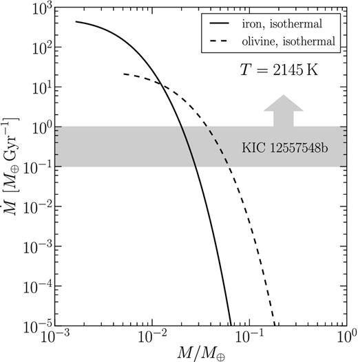
Mass-loss rates |$\dot{M}$| computed using the isothermal model at T = 2145 K, for iron planets and olivine planets of varying M. In the low-M, free-streaming limit, the higher vapour pressure of iron allows for a higher |$\dot{M}$| than for olivine. At larger M, mass-loss rates are lower for iron planets than for olivine planets because of the higher molecular weight of iron. Our estimate for the maximum present-day mass of KIC 1255b varies by a factor of 2 between the iron and olivine scenarios.

Figure 11.

Open in new tabDownload slide

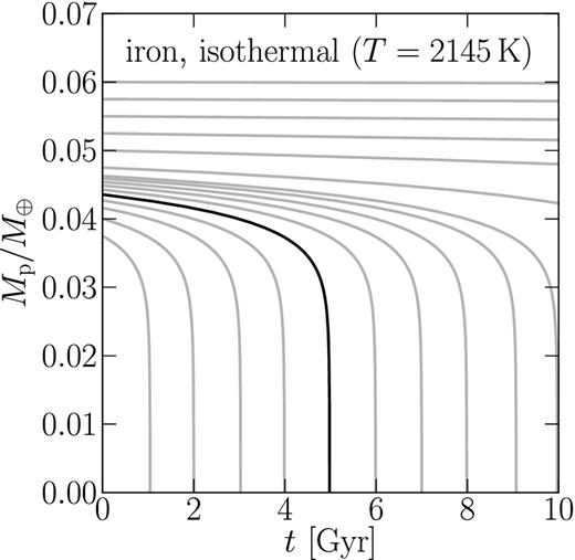
Mass-loss histories M(t) for an iron planet, obtained by time-integrating |$f_{\rm {duty}} \cdot \max \dot{M}$| with f_duty = 0.5 for an isothermal wind. An iron planet with a 5 Gyr lifetime will have an initial mass of ∼0.044 M_⊕. As was the case for olivine planets (see Fig. 9), the catastrophic evaporation stage lasts only for ∼100 Myr. Iron planets (or planetary iron cores) with masses greater than 0.05 M_⊕ survive for over 10 Gyr.

According to Fig. 11, iron planets with M ≳ 0.05 M_⊕ survive for tens of Gyr. Compare this result to its counterpart in Fig. 9 (left-hand panel), which shows that olivine planets with M ≲ 0.1 M_⊕ evaporate within ∼10 Gyr. This comparison suggests that for planets with the right proportion of silicates in the mantle to iron in the core, mantles may be completely vaporized, leaving behind essentially non-evaporating iron cores. Such massive, quiescent iron cores might be detectable by Kepler via direct transits (see Section 4.6).

4.8 Dust condensation

Recall that we have not modelled the microphysics of dust formation, but treated the dust-to-gas ratio as a free function. Are the conditions of our flow actually favourable for the condensation of dust? Any gas whose partial pressure is greater than its vapour pressure (at that T) might condense and form droplets (modulo the many complications discussed below). Condensation might proceed until all vapour in excess of saturation is in cloud particles. If the condensates have sedimentation velocities larger than updraft speeds, they will rain out of the atmosphere; otherwise, they remain aloft (see e.g. Lewis 1969; Marley et al. 1999; Ackerman & Marley 2001; Helling et al. 2001).

In Fig. 12, we compare gas pressures of our solutions (for |$\dot{M} = \max \dot{M}$|⁠) at M = 0.01, 0.03 and 0.07 M_⊕ with the equilibrium vapour pressures of olivine and pyroxene. At the base of the flow, the gas pressure equals the saturation vapour pressure of olivine by construction. As gas expands and cools, its pressure generally remains above the saturation pressure of pyroxene, so conditions are favourable for the condensation of pyroxene grains. Unfortunately, we have an embarrassment of riches: at T ≲ 1700 K, our gas pressures are many orders of magnitude higher than silicate vapour pressures, and the concern is that gas condensation will lower pressures precipitously to the point where winds shut down. This fate could be avoided if grains take too long to condense out of the outflowing and rapidly rarefying gas – i.e. the finite time-scale of grain condensation might permit gas to remain supersaturated. Furthermore, even before bulk condensation can begin, seed particles must first nucleate from the gas phase. These issues call for a time-dependent analysis of grain formation, perhaps along the lines made for brown dwarf and exoplanet atmospheres (Helling et al. 2001, 2008a,b; Helling & Rietmeijer 2009). Accounting for the extra heating from small grains with sizes ≪1 μm as they first condense out of the wind (Section 4.2) would keep the gas closer to isothermal and help to prevent catastrophic condensation.

Figure 12.

Open in new tabDownload slide

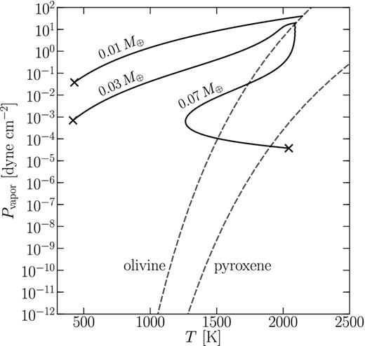
Trajectories of the wind in pressure–temperature space, computed using the full model for M = 0.01, 0.03 and 0.07 M_⊕. Gas pressures generally remain above the equilibrium vapour pressures of pyroxene, permitting the condensation of pyroxene grains.

Of course, by the time the wind leaves the sonic point and is diverted into the trailing comet-like tail, it must be full of grains to explain the observed occultations of KIC 1255b. In this paper, we have not modelled the dusty tail at all. Future work should address the dynamics of the tail and compute its extinction profile, with the aim of reproducing the observed transit light curves.

5 CONCLUSIONS

Our work supports the hypothesis that the observed occultations of the K star KIC 12557548 originate from a dusty wind emitted by an evaporating planetary companion (‘KIC 1255b’). We reach the following conclusions.

• Maximum present-day mass. Our estimates for the maximum present-day mass of KIC 1255b range from max M ≈ 0.02 M_⊕ (roughly twice the mass of the Moon) to max M ≈ 0.07 M_⊕ (slightly larger than the mass of Mercury), depending on how strongly the wind is heated by dust and can remain isothermal (Fig. 8). For these maximum masses, calculated mass-loss rates peak at |$\max \dot{M} \sim 0.1$| M_⊕ Gyr⁻¹, which is just large enough to produce the observed transit depths of the order of 1 per cent. Smaller planets with weaker gravities yield larger mass-loss rates and are also compatible with the observations.

• Maximum formation mass. For an assumed planet age of ∼5 Gyr, the maximum mass of KIC 1255b at formation ranges from 0.06 to 0.1 M_⊕, again depending on the energetics of the wind (Fig. 9).

• Mass threshold for catastrophic evaporation. A pure rock planet of mass ≳ 0.1 M_⊕ and surface temperature ≲2200 K will survive with negligible mass-loss for tens of Gyr.

• Time variability. The observed occultations of KIC 12557548 vary by up to an order of magnitude in depth without any apparent correlation between orbits. The implied order-of-magnitude variations in |$\dot{M}$| can be explained in principle by the exponential sensitivity of |$\dot{M}$| to conditions at the planet surface. The dynamical ‘refresh’ time-scale of the wind t_dyn ∼ 14 h is similar to the orbital period P_orb = 15.7 h. This supports our dusty wind model because were t_dyn ≫ P_orb or t_dyn ≪ P_orb, then eclipse depths would correlate from orbit to orbit, in violation of the observations.

• Progenitors and occurrence rates. KIC 1255b's current catastrophic mass-loss phase may represent only the final few per cent of the planet's life. As such, for every KIC 1255b-like object, there could be anywhere from 10 to 100 larger planets in earlier stages of mass-loss. These close-in, relatively quiescent progenitors may be detectable by Kepler through conventional ‘hard-sphere’ transits if they are as large as Mercury. We cannot, however, rule out the possibility that the progenitors are lunar sized or even smaller. If KIC 1255b remains the only catastrophically evaporating planet in the Kepler data base, then the occurrence rate of close-in progenitors orbiting K stars with sub-day periods is >0.1 per cent, with larger occurrence rates for progenitors increasingly smaller than Mercury.

• Iron planet. KIC 1255b may have lost ∼70 per cent of its formation mass to its thermal wind. It seems possible that today only the iron core of KIC 1255b remains and is evaporating. Transmission spectra of the occulting dust cloud might reveal whether the planet's surface is composed primarily of iron or silicates.

• Future modelling and observations. Keeping the wind hot as it lifts off the planet surface significantly enhances mass-loss rates. In our model we have included heating of the gas by micron-sized grains embedded in the flow. But these grains can also shadow the surface from starlight and reduce |$\dot{M}$| if they are too abundant. Additional heating may be provided by super-blackbody grains with sizes ≪1 μm which do not significantly attenuate starlight. Future models should incorporate such tiny condensates – and treat the dusty comet-like tail that our paper has completely ignored. More information about grain size distributions and compositions might be revealed by Hubble observations of KIC 12557548 scheduled for early 2013.

We thank Saul Rappaport for alerting us to the feasibility of detecting Mercury-sized progenitors of KIC 1255b using Kepler, and Andrew Howard and Geoff Marcy for sharing their Keck observations of KIC 12557548. We are also grateful to Andrew Ackerman, Tom Barclay, Bill Borucki, Raymond Jeanloz, Hiroshi Kimura, Edwin Kite, Michael Manga, Mark Marley and Subu Mohanty for useful and encouraging conversations; to Paul Kalas for pointing us to work on beta Pictoris that presaged the story of KIC 1255b; and to an anonymous referee for a helpful report that motivated us to review the various modelling uncertainties and introduced us to the cloud formation literature. DPB acknowledges the support of a UC MEXUS-CONACyT Fellowship. EC acknowledges Hubble Space Telescope grant HST-AR-12823.01-A.

REFERENCES