Quantitative Finance
Published January 2017
•
Copyright © IOP Publishing Ltd 2017
Pages 1-1 to 1-17
You need an eReader or compatible software to experience the benefits of the ePub3 file format.
Download complete PDF book, the ePub book or the Kindle book
Permissions
Abstract
Quantitative finance is a field that has risen to prominence over the last few decades. It encompasses the complex models and calculations that value financial contracts, particularly those which reference events in the future, and apply probabilities to these events. While adding greatly to the flexibility of the market available to corporations and investors, it has also been blamed for worsening the impact of financial crises. But what exactly does quantitative finance encompass, and where did these ideas and models originate? We show that the mathematics behind finance and behind games of chance have tracked each other closely over the centuries and that many well-known physicists and mathematicians have contributed to the field.
Introduction
At first glance, the term 'quantitative finance' seems rather over-specified, for surely finance is by its nature based on calculations. But in recent decades this phrase has come to describe a fairly well-defined set of methods and mathematical models that are used to value and trade a large set of complex transactions which take place throughout the global financial markets. These transactions are entered into by companies to facilitate trade and investments, and by governmental bodies to achieve policy aims. A second and related branch of quantitative finance is the mathematics underlying the construction and characteristics of investment portfolios. Finally, not always included in the true 'quantitative finance' category are the risk-management processes used by large financial institutions to try to ensure that the risk of large losses in the portfolios of transactions that they hold is low.
Recent years have seen a growth in courses and qualifications in quantitative finance, and it has become a chosen profession of many mathematics and science graduates. Several hundred textbooks cover different aspects of the field, and multiple specialist journals publish papers in the area. However, the financial crisis of 2007/8 cast a shadow over the field, as the crisis was quite probably worsened by many complex transactions whose multifarious and entangled risks were far larger than anticipated, and almost impossible to determine. While crises caused by herd behaviour and market bubbles are not new, quantitative finance certainly added a new ingredient to the mix.
The employers of quantitative finance specialists, or 'quants' as they are known, are in general large financial institutions, like investment banks, hedge funds, insurance companies, and sometimes governmental bodies like central banks or sovereign wealth funds.
Why should we care about this relatively new branch of applied mathematics? The answer is that it has come to affect all our lives. Pension portfolios are constructed and risk managed using quantitative finance methods. Companies with overseas investments and cashflows rely upon it. Mortgage products beyond simple floating rate interest are only possible because of quantitative finance methods. Insurance companies invest and risk manage their premiums using quantitative finance. Each trading day, literally trillions of US dollars' worth of money flows through the global marketplace, governed by quantitative finance calculations.
This enormous leap in traded volumes from a few decades ago has been partly facilitated by the development of quantitative finance techniques, but mostly due to the growing use of electronic trading. While electronic trading has enabled transactions to be executed far more smoothly and quickly than was ever the case before, this very ease and degree of automation means that it has come under criticism for allowing huge numbers of trades to take place whose purpose is only to make profit margins from market movements; for example, a tendency to reverse direction after a certain move could be exploited by an automatic algorithm. This type of 'algorithmic trading' where automated systems execute transactions without human intervention is blamed for causing some types of market instability and 'flash crash' episodes.
There is no doubt that at their best, quantitative finance techniques facilitate global trade and investment. Consider a European car maker that sells vehicles to the US and Asia. The firm's expenses are in Euros, its profits in other currencies. Quantitative finance techniques mean that the company can pay a premium to insure itself against unfavourable currency variations. This type of transaction was much more difficult—perhaps impossible—to create and value prior to the advent of quantitative finance methods. However, at their worst, they can be misused to mean that market participants are left with unknown—and unacceptable—levels of risk, often hidden behind blinding levels of complexity.
What could the future be for the field? This lies more in the realm of regulation than mathematical innovation. A level playing field where the undoubted benefits of quantitative finance can be easily delivered to market participants is highly desirable, but can it be accomplished while ensuring that it is not misused?
Background
The story of quantitative finance is partly the story of mathematics. As mathematics advanced, its concepts were taken up and used in the financial world. It is popular to date 'ground zero' of quantitative finance to around 1973, when Fischer Black, Myron Scholes and Robert Merton published papers introducing a new framework for the valuation of financial instruments [2, 3]. But this is unfair to history and omits the branch of quantitative finance concerned with portfolio construction.
Possibly the very first contender for the job of 'quant' was a wonderful philosopher from Ancient Greece, called Thales, believed to have been born in 625 BC. Many of the surviving writings of the time mention him; he seems to have had many talents, from geometry to engineering. Sadly none of his own writing survives. According to Aristotle [4], Thales predicted a good olive harvest later in the year, and put down deposits to hire all the olive presses in the region at that time. He could then let them out at a high price when the harvest came. This is a perfect example of buying an option contract; a limited outlay for a potentially very high gain. An option is the right, but not the obligation, to buy or sell an underlying asset or market instrument (like a share, or an amount of currency) at a specified price (called the strike price) at a specified date or range of dates in the future. The price paid for this right is called the premium.
The first book that can truly be said to include quantitative finance was called Liber Abaci, or the Book of Calculations, by Fibonacci [5], in Italy in 1202, though only the 1227 version survives. This was also the book that introduced Arabic numbers to Europeans, who up until that time had been struggling to do arithmetic with Roman numerals or a Greek abacus when things got difficult. Liber Abaci introduced some critical elements of quantitative finance, including currency conversions, the time value of money and interest rates, 1 and the law of one price 2 .
The next important text combines quantitative finance and gambling (perhaps the first time this association was made, but certainly not the last!). It is Liber de Ludo Aleae, or the Book of Games of Chance, by Girolamo Cardano and was published in 1663, though thought to have been written about 1565 [6]. Galileo wrote about die-throwing in the early 1600s and seems to have read a copy of Cardano's work. It introduces some of the fundamentals of probability; for example, when discussing the casting of a six-sided die, he says 'in six casts each point should turn up once, but since some will be repeated, it follows that others will not turn up'. A century later, Pascal and Fermat [7] made further advances in probability theory using die throws and began the science of valuation by calculating what bets were worth making on the result of different throws. The subject was becoming popular, with Christian Huygens also publishing a review of the area [8]. The Bernoulli family took up the baton in the 17th and 18th centuries, and Abraham de Moivre published the third edition of his book the Doctrine of Chances in 1756 [9]—gambling again—which develops much of modern probability theory and brings in financial mathematics with the calculation of the value of annuities.
If I had to myself choose the 'beginning' of the field of quantitative finance, I would not, I think, be alone in selecting the publication in 1900 of the doctoral thesis of a student at the Sorbonne called Louis Bachelier [10]. He had derived the mathematics underlying Brownian motion 3 , and used them to explain the movements of the stock market, and value stock option contracts. In a wonderful coincidence, Albert Einstein published almost the same solution in 1905, although he used it to advance the theory of thermodynamics and determine the size of atoms. Both seem to have been unaware of the other's work. The similarity underlying all these phenomena is the central limit theorem, which means that when there are enough random uncorrelated influences acting on a variable (like the position of a pollen grain in water, or the value of a stock in an active market) that the values of the variable over time will be distributed according to a normal distribution. Of course, harking back to all the history with gambling, the probability of getting a given number of heads or tails in a series of coin throws is also normally distributed, as long as there are very many throws.
From this point, development of quantitative finance was fairly swift. The Russian mathematician Andrey Kolmogorov introduced the idea of conditional expectations in a paper in 1933 [11], and Kiyoshi Ito laid the foundations of stochastic calculus in his papers in 1942 and 1951 4 [12, 13]. Case Sprenkle (1961) [14] adapted Bachelier's work using 'lognormal' returns 5 , James Boness (1964) [15] introduced discounting, and Paul Samuelson (1965) [16] allowed the option to have different risk levels than the stock. Robert Merton, a student of Samuelson, worked on the theory with Black and Scholes, and finally now we arrive at the 1973 [2] publication of the Black–Scholes–Merton model which sparked off the still-growing trading of financial derivatives products. Quantitative finance had arrived.
Somewhat in parallel to these developments, Harry Markowitz kicked off the field of portfolio selection in 1952 [17]. Before he took a statistical approach to building portfolios, they were simply collections of individual stocks, selected for desirable properties. He realised that the overall risk and return of a portfolio could be hugely improved if the construction of the portfolio took correlations into account—the variation in overall value could be reduced per unit of return. In a way he was only doing what insurance companies have done for many years—pooled risk—but it had never been scientifically applied to portfolio management before. He came up with the concept of the 'efficient' portfolio—the set of portfolios yielding the highest expected returns for different levels of risk. Other contributions to the field of asset management were the capital market line (James Tobin) [18] and William Sharpe's development of the Capital Asset Pricing Model [19].
If not ground zero, we can certainly mix our metaphors and call 1973 the Big Bang of quantitative finance. What has happened since then? An initial period of expansion saw the Black–Scholes–Merton model extended to other markets like interest rates (Robert Merton 1973) [3] and Foreign Exchange (Mark Garman 1982) [20]. However, in 1987 the S&P 500 index fell by over 20% of its value in a day, and some of the shortcomings of the model were laid bare. Central to the foundation of the model was the assumption that market prices are lognormally distributed. Yet the move in the S&P was so large as to have a probability of pretty much zero, according to the lognormal distribution. What was going on?
It was quickly realised that the distribution of market rates is only imperfectly modelled by the lognormal distribution. The actual distributions have 'fat' tails and large moves are unexpectedly likely to occur. The 1987 crash led to a set of new mathematical techniques designed to cope with this fact. Other developments began to account for different observations of market behaviour, like the fact that interest rates tend to stay in a range, or that the standard deviation of market distributions is not constant. In the 2000s credit joined the set of market rates which were becoming actively traded, and whose derivatives were being valued with highly quantitative methods.
Coupled with a wave of deregulations of the financial industry, which allowed high-street lenders to merge with investment banks and acquire innovative products (and their risks), the stage was set for the 2008 financial crisis. A bubble in the American housing market became more than just a local problem as the new credit derivatives allowed investors all over the world to indulge in the time-honoured practice of believing that what goes up, can go on up forever. The regulatory bodies were way behind the curve and not capable of assessing the risks of the products. And the quants who built them were not the managers who pushed the sales force to sell more and more of them. This disastrous division of roles—exacerbated by the insular tendency of scientists and mathematicians to focus on problems they know how to solve—has been well described in Riccardo Rebonato's book [21]. The quants who were busy designing products that were almost bound to fail thought that someone senior surely knew what they were doing—when the management level was more focussed on the profitability of the area. As has been said before, bubbles and irrational investors are nothing new. But a combination of increased access to markets and new high risk products meant that this bubble was very large, and very hard felt when it burst.
Since this rather inglorious period, developments in the quantitative finance field have been steady. Some models focus on including jumps and large moves within their framework. A new challenge which the last few years has brought is that of negative interest rates, which required modification of many interest rate models and abandonment of others. Regulatory initiatives are being implemented which aim to prevent another similar crisis, but it remains to be seen whether they are constructed with sufficient understanding of the area to achieve their aims.
Current directions
We now take a brief look at two areas of topical interest in quantitative finance today; negative interest rates, and anomalies in the foreign exchange market.
Negative interest rates
In 2015, an extraordinary thing happened in Europe. Short- and medium-term interest rates dipped below zero into negative territory, driven by a central bank desperate to stimulate the stagnant economies of the region 6 . So unlikely was this thought to be, that many interest rate models had to be quickly adjusted, and some had to be abandoned. The only recent previous example of such a situation had been a brief flirtation with negative rates by Switzerland in 1979, and this was assumed to be a temporary aberration. But as can be seen from figure 1, this time it seems to be here to stay.
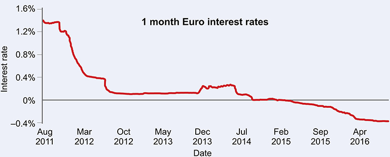
Figure 1. Short-term interest rates in Europe drift below zero. Data source: Bloomberg.
Download figure:
Standard image High-resolution imageThis is a quite unparalleled situation and there is little in recent history to guide us. What does it really mean? That we have to actually pay money to have money on deposit? That we get paid money to borrow? Extraordinary!
The answer is that the simplistic assumption that rates cannot go below zero is not quite true. Years ago, the concept of paying the bank to store your valuables was quite accepted (thus implying an effective negative rate). Today, investors that are facing negative interest rates cannot easily convert their sizable holdings into cash, or face a significant cost or risk when doing so 7 . Thus the costs of storing and transporting cash comes into consideration, including the premiums that would be charged to insure large amounts of physical banknotes. These various costs indicate that the effective lower bound of interest rates can certainly be slightly negative. But even beyond this, there is not nearly enough physical cash in any economy to allow many of the large depositors to actually hold their investment in banknotes. And a central bank intent on a negative rate policy will not have any incentive to print more!
Of course, the man or woman in the street will not experience negative interest rates. That would be a recipe for instant withdrawals of cash, which no-one wants to see. Rather, it is a situation that affects deposits that large banks hold with their central bank, or very large investors. So far banks have been reluctant to pass this cost on to their clients, though it could certainly be a possibility for very large depositors if rates slide further. Clearly there is a fairly hard limit which rates cannot slip below, where depositors begin to explore other ways of storing their money. So a rapid evolution of interest rate models began.
Interest-rate models have always been a slightly special case. Their behaviour is quite distinct from that of stocks or commodities; in normal times they have a stable range that they rarely exceed and tend to revert to. Additionally, it is desirable to preserve the 'arbitrage-free' 8 nature of the term structure. To understand what this means, consider a request from a client to a bank, asking what rate the bank would guarantee for a three-month deposit beginning not today, but three months in the future. To calculate this guaranteed rate, the bank will look at the current three-month rate, and the current six-month rate. As shown in figure 2, there are two ways of the bank locking in deposits for six months; the first is simply to enter an agreement to deposit the money for that time (r06 below). The other is to agree now to invest now, for three months, and also agree now to deposit the initial amount plus earned interest of that deal into a second three-month investment, beginning just as the first concludes (r03 and r36 below). If these two processes (three-month deposit starting now plus three-month deposit starting in three months versus a six-month deposit starting now) are not equivalent, then it is simple to see that one could 'round trip' the process and make some risk free profit at the expense of the hapless bank!
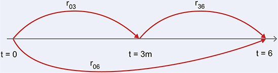
Figure 2. There are two ways of the bank locking in deposits for six months; the first is to enter an agreement to deposit the money for that time (r06). The other is to agree now to invest now, for three months, and also agree now to deposit the initial amount plus earned interest of that deal into a second three-month investment, beginning just as the first concludes (r03 and r36).
Download figure:
Standard image High-resolution imageSo as the principle of no free money — 'no arbitrage' — is one of the fundamental facts of the market, a relationship between these rates is established and maintained. Now, when one considers that one can invest for any reasonable period, and that these 'forward rates' like r36 are liquidly 9 traded in the market 10 , one can see that the interest rate curve can only evolve in a constrained manner, and models that embody these constraints are very useful, both to investors and corporations who want to invest or borrow, and to banks who have to set the rates for these contracts.
Thus from the start of the market, interest rate models have been somewhat modified to account for these unique features. The early models, like those of Robert Merton (1973) [3] and Oldrich Vasicek (1973) [22] tended to model the 'short' interest rate (the theoretical rate for a very short term investment). As the area developed, models expanded their scope to include the forward rate curve, by which I mean the various rxy described above (known collectively as Heath–Jarrow–Morton type models) [23]. Later developments allowed more realistic behaviours to be represented (allowing flexible distributions, for example, or introducing correlations between observed market variables). Below we give a general descriptive formula to show how interest rate models tend to work.
To represent the bounded nature of interest rates, models tend to include
either some kind of mean reversion (e.g. Vasicek, Cox–Ingersoll–Ross
[24],
Hull–White [25]), or to have a lognormal distribution (e.g.
Black–Derman–Toy [26], Black–Karasinski
[27]). Sometimes an additional equation is needed to represent
the model; for example, the Chen [28] model has a stochastic
mean and volatility which are separately defined, and these are referred
to as multi-factor models. Download figure:
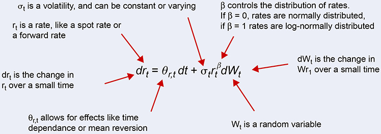
In general, a lognormal distribution fits observed rates better than an explicit mean reversion factor, and has historically been preferred as it naturally precludes rates going below zero (once such a desirable feature!). The normal model will allow rates below zero, for suitable mean and volatility, but the lognormal will not.
Valuing interest rate contracts under negative rate scenarios
For simple contracts, negative interest rates are not a problem (at least mathematically!). If they directly reference a negative rate, a cashflow (from party A to party B) simply reverses direction (from party B to party A)—in other words, a profit becomes a loss, a receipt becomes a payment, and so on. It may not be expected, or welcome, but it is not difficult to calculate.
More complex products, however, do have problems when negative rates arise. This comes from the models that are used to value products whose cashflows depend on rate levels and movements after the start date—in other words, option-like products. When such a product is to be valued, it is essential to have a model of interest rates that includes the probability of those rates taking various values in the future—that is, the model must include a probability distribution of interest rates. When the probability of different outcomes can be calculated, the value of the product is found by adding together all the possible outcomes multiplied by their probabilities. The problem comes when we realise that many commonly used interest rate valuation models, as discussed above, apply a probability of zero to negative rate scenarios!
Additionally, many contracts apply a legal cap or floor at zero to the contract. It was probably envisaged that these clauses would only be invoked in the case of severe market disruption, but the effect upon the contract is to lend option-like characteristics to even a previously linear product.
The SABR model; state of the art
The Stochastic Alpha Beta Rho (SABR), developed by Patrick Hagen and colleagues, first came on the scene in 2002 [29], and was immediately popular. It allows volatility (defined as the standard deviation of the distribution) to itself be a stochastic variable, and additionally introduces a correlation between the forward rates and the volatility. Finally, the parameter σ, which defines the distribution, is also a variable that may be fitted to market data. This flexibility means that explicit mean reversion becomes unnecessary.
Its evolution is defined as below:
Here Ft is the forward rate, σt is the volatility, W and Z are random processes, α is the volatility of the volatility (sometimes called the volvol) and ρ is the coefficient of correlation. However, one fly in the ointment remains; the parameter β is forced to be zero if rates are negative or close to negative, thus removing one of the attractive pieces of flexibility of the model. The solution is the SABR model with an additional displacement factor s, as below [32]:
This has now become the best market practice to accommodate negative or near-negative rate environments, and gives flexible distributions, as illustrated in figure 3.

Figure 3. Probability Distribution using SABR model. Data source: [31]. Reproduced with permission.
Download figure:
Standard image High-resolution imageAnomalies in the Foreign Exchange market
The Foreign Exchange market is the largest in the world. Every trading day, over 5 trillion US dollars' worth of flow goes through it. It trades 24 h a day. The Foreign Exchange (FX) options market alone trades 250bn US dollars' worth of flow per day. It dwarfs other global markets (figure 4).

Figure 4. Daily global USD equivalent traded flow of FX options Data source: Bank of International Settlements Triennial Survey 2016 http://www.bis.org/publ/rpfx16.htm
Download figure:
Standard image High-resolution imageIt is used to trade, to invest, and to speculate. One reason for its dominance is that many trades of other types involve FX by their nature—for example, buying an overseas share index will naturally incorporate an FX transaction. Companies that have overseas subsidiaries will have income in other currencies. Various commodities are quoted in particular currencies (usually the US dollar). So the market is heavily scrutinised and studied.
One might imagine, then, that it is ruthlessly efficient, and that trading strategies that exploit predictable patterns in it would be non-existent. But bizarrely, this is not so. The first piece of evidence for this startling fact is the FX carry trade.
The FX carry trade
To understand where this comes from, we can go back in time a little to the formation of the FX market. In its current free floating form it is young, born in the 1970s as one by one exchange rates broke free from various pegs and controls and traded freely. It was assumed that these new floating rates would have their underlying value determined by interest rates and inflation in their own country. This led to the idea of Uncovered Interest Parity (UIP)—that FX rates will on average track the forward rates determined by the relative interest rates between two countries. This forward rate is simply the current rate adjusted for interest rate effects. To understand how it works, we can consider (just as for interest rates) asking a bank for a guaranteed FX rate at a future date. There are two ways of getting from one currency at the start of the period, to the other currency at the future date.
- (1)Exchange now, and invest the foreign currency at the foreign interest rate for the period up to the future date
- (2)Invest the home currency now for the period up to the future date, then exchange
The final exchange in (2) is the rate you are asking the bank to
guarantee. If we stick to the principle (and we can) of
no-arbitrage, then the proceeds of (1) and (2) must be equal, or
there will be a risk free profit to be made somewhere. Given that we
know all of the current FX rate, and the two interest rates, we
should be able to calculate the forward FX rate. An example is given
below for euro and the US dollar. Download figure:
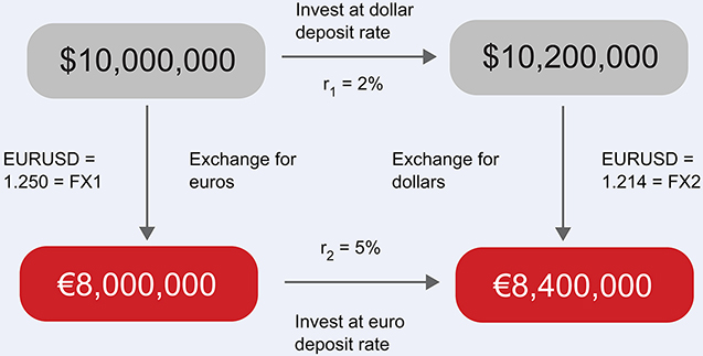
Thus we have
And by putting in the numbers, you can see that FX2, the forward FX rate, must be 1.214. Note that the interest rates are not those of today, which are close to zero or even negative; for clarity, they are those of a few years ago!
Now, the bank is constrained to offer this and only this rate as the forward guaranteed FX rate—or it leaves itself open to arbitrage—but this does not necessarily mean that it is a good forecast of the future. In fact, the forward rate is a poor forecast and contains no information about the size or direction of future FX moves. Thus, by systematically betting against this move, on average, one can generate money over time. Figure 5 shows the percentage returns of the amount of money exchanged (notional amount), if this strategy were pursued on a quarterly basis over all developed markets, since 1987. The black line is the actual profit, the forward point component is the profit purely due to the interest rate difference, the FX component is the profit due to the FX rate moves, and the UIP path is the profit (or loss) that would have been made had the FX rates always moved to the forward rate, as UIP would predict.
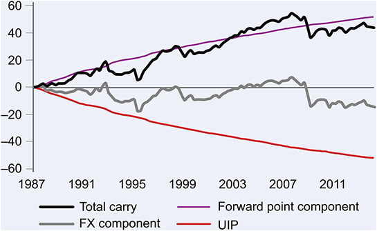
Figure 5. Carry trade in FX, from the 1980s, averaged over all liquid currency pairs. Data source: [30]. Reproduced with permission.
Download figure:
Standard image High-resolution imageWhen one considers that the capital at risk in this trade is much less than the notional amount, then it is clear that this could be a very useful trading strategy. It is known as the FX carry trade and some organisations have traded it profitably for many years.
But how can this be so? The largest market on the planet seems to be significantly inefficient!
There are several reasons that this trade persists. It is not risk free; the 2008 crisis caused severe losses. But also, the FX market is perhaps the only one where many trades are executed without regard to their eventual profitability; they are often part of other transactions and need to be executed regardless. And FX rates are subject to many pressures; the carry trade is only a very small part of their overall movement.
FX option anomalies
As we might expect, the market for options on FX rates is also very large. FX options are the most widely used derivatives in the world, with trades for many and diverse reasons. From long term hedges of overseas income, right through to opportunistic option selling, they are used as protection, as positioning tools, and as profit generators.
But are they good value? Are they too cheap, or too expensive? There is no consensus agreement on this, and much rumour! Corporations may be convinced that they are paying too much for protection. The investors may be wary of using them to deliver returns because they do not know if they are biased to be cheap or expensive. Though this seems extraordinary, the focus of the markets and the traders is always in the 'now' and the near future; historical data are not usually considered to be important. There are very few studies available where the end value of contracts is compared systematically to their initial cost, and the answers can be revealing.
One such published study was conducted by the author [30]. It became apparent during the course of the study why it had not often been attempted before, as the data were difficult to source, clean and analyse. But after some effort, it was possible to compare the original price of the FX options (the premium) with the eventual payout. In an efficient world, the premium and payout would be very similar, with no systematic difference. Instead, what was discovered was that there are significant, long term differences. Figure 6 plots premium/payout as a function of the term of the options, which range from one week to three years.

Figure 6. Payout/premium ratio for FX options, aggregated over G10 and EM currency pairs. Put options are options to sell, call options are options to buy. Data source: [30]. Reproduced with permission.
Download figure:
Standard image High-resolution image
To obtain this graph in the original publication, we used data from Bloomberg—one of several data vendors from whom historical data can be sourced. There were 34 available currency pairs with data from 1995 for the longer data series. Trading costs were included at all times. Weekly data were used to calculate the premiums of the options, and then the calculation looked forward to the expiry date of the options to calculate the option payout. A discount was applied to the payout to recognise the fact that it occurs at a different point in time from the premium. Finally, for each option, the payout was divided by the premium to discover whether the option overall made or lost money. The average of these payout/premium calculations, averaged once more over currency pairs in the G10 bloc and in the non-G10 Emerging Market (EM), is what appears on the graph. If the market were perfectly efficient, we would expect these points all to lie approximately on the 100% line. (Although this is strictly true only in a 'risk-neutral' world, nevertheless a situation where money can be made with a systematic trade is not expected in a liquid market.)
We see that the options are far from an efficient market. Call options (options to buy the currency) are worse value in the longer tenors, paying back as little as 50% on average of their cost, while put options (options to sell the currency) can pay back up to 130%. Emerging market currencies show the strongest effect in both puts and calls. This is an absolutely unexpected result, and it was extraordinary that it had gone unnoticed for so long.
Once noticed, however, the explanation may be derived from the data. Looking at the currency-by-currency results gives us a clue. The US-dollar and Australian-dollar (USD-AUD) currency pair is a glaring outlier. Where the average payoff/premium ratio for all the calls for the three-year tenor is 41%, the pair comes in at 180%, by far the highest. For the puts, the 3Y tenor for the AUD is 12%, in complete contrast to the average of 127%. This leads us in the direction of the answer. The AUD currency on average has had much higher interest rates, over time, than the USD. Most of the currency pairs in the sample are the other way round—in general, the USD or the euro (EUR) are the base currency, and in general they have lower interest rates than the other currency in the pair. But AUD is the notable exception; other pairs where a similar effect has occurred would be those involving the Japanese yen (JPY), like USD/JPY or EUR/JPY, as the JPY has had a very low interest rate regime for many years—and these pairs too, show unusual behaviour. And finally, the EM pairs, which show the strongest effect, have on average the highest interest rates.
The answer to the puzzle is that the interest rate differentials give rise to the forward rate, which is assumed in the option pricing process to be the best forecast for the future FX spot rate. The forward rate predicts that the higher interest rate currency will fall in value relative to the lower. This (usually) is the same as saying that the FX rate will go up. So if it does not go up as much as predicted, puts (option to sell the rate) will make money and calls (option to buy the rate) will lose money. And for currencies like AUD/USD or USD/JPY, it will be the other way round. This is exactly what we see.
Incredibly, no-one has noticed this up till now. But the corporations of the world should surely be told that some of the hedge contracts they are contemplating have historically been much better value than others. The investors of the world can suddenly have a much better idea where value lies in the FX option space.
Outlook
Where is the quantitative finance field going? There is no shortage of highly intelligent financial engineers—mostly from physics, mathematics or engineering backgrounds—eager to devise new and more beautiful mathematical models, capable of valuing ever more esoteric products, but to blindly continue down this path would be to ignore the lessons of the financial crisis. Regulatory pressure is bearing on the industry; though the various new directives which are currently under discussion and implementation may be imperfect, they stem from the strongest possible desire to ensure that quantitative finance techniques are never again used in such a manner that they exacerbate a global crisis. This aligns perfectly with the view of the author that it is unwise to focus too closely on models which are mathematically tractable at the expense of the accuracy of their description of the market. Put bluntly, folk need to take a look at the data.
Hence, my choice of detailed examples has included the analysis of FX options, which to some more traditional 'quants' would be somewhat peripheral to the quantitative finance field. But in my view, it is essential that finance be studied in an 'evidence-based' fashion if it is to be of benefit to the economies of the future.
Central to the discussion is the use of 'implied' quantities, like the forward rate. These are 'forecasts' of market quantities that are embedded in and essential to the mathematics of valuation. Other implied quantities can be probability of default, correlation of different markets rates, and many more. The fact that they may well not be good estimates of the future is usually taken to be irrelevant, and indeed, the way that trading desks hedge their portfolios tends to ensure that they are not relied upon in this way. But, when they become too far detached from reality, as they did when they were used to enable unemployed people in the US to acquire multiple mortgages with no detailed scrutiny, then something is wrong.
The case of the FX options, where a huge liquid market got it badly wrong over several decades, is not unusual. There are multiple markets where this kind of study could be done—but nobody is doing this work. The author feels that the future of the field lies in transparency and analysis of data alongside the development of mathematical techniques.
This can only benefit corporations and investors, and only penalise those who design products which are not fit for purpose. As market spreads reduce, more complex products have the potential for generating higher returns for their designer—but is this beneficial to the end user? Complexity for the sake of complexity has no utility.
But here, paradoxically, spread compression and commoditisation of financial products has played a part. As profit opportunities in normal business reduce, other avenues are naturally sought out to replace them, possibly not to the benefit of the buyer. We may make an analogy with free retail banking; it's not feasible to run a retail bank where no-one pays for their account. Someone, somewhere will pay, even if these fees are for unauthorised overdrafts or other minor misdemeanours.
It is not clear what the answer should be, or whether the new regulations fully grasp the current problems. We must hope that as the markets mature and evolve, these issues can be resolved in a way which retains the enormous power and flexibility of the quantitative finance world, while keeping risks well under control.
References
- [1]Lightner O C c1922 The history of business depressions The Northeastern press—2010 reprint available
- [2]Black F and Scholes M 1973 The pricing of options and corporate liabilities J. Political Economy 81 637–54
- [3]Merton R C 1973 Theory of rational option pricing Bell J. Econ. Manage. Sci. 4 141–83
- [4]Steele C (ed) 2015 Metaphysics Alpha (Oxford: Oxford University Press) Aristotle
- [5]Pisano L 1227 Fibonacci's Liber Abaci: A Translation into Modern English of Leonardo Pisano's Book of Calculation (New York: Springer) (Fibonacci) translated by Laurence Sigler 2002
- [6]Cardano G (ed) 1663 The book on games of chance: (Liber de Ludo Aleae) (New York: Holt, Rinehart and Winston) translated by Sydney Henry Gould
- [7]Devlin K 2010 The Unfinished Game: Pascal, Fermat, and the Seventeenth-Century Letter that Made the World Modern (New York: Basic Books)
- [8]Gullberg J and Hilton P 1997 Mathematics from the Birth of Numbers (New York: Norton)
- [9]de Moivre A 1756 The Doctrine of Chances: or, a Method of Calculating the Probabilities of Events in Play 3rd edn (: (Andesite Press) reprinted 2015
- [10]Bachelier L, Samuelson P A, Davis M and Etheridge A 2006 Louis Bachelier's Theory of Speculation: the Origins of Modern Finance (Princeton NJ: Princeton University Press)
- [11]Kolmogorov A 1956 Foundations of the Theory of Probability 2nd edn (New York: Chelsea Publishing Co.) Translation (1960)
- [12]Kiyosi I 1942 On stochastic processes (infinitely divisible laws of probability Japanese Journal of Mathematics 18 261–301
- [13]Kiyosi I 1951 On a formula concerning stochastic differentials Nagoya Mathematical Journal 3 55–65
- [14]Sprenkle C 1961 Warrant prices as indicator of expectations and preferences The Random Character of Stock Market Prices , ed P H Cootner (Cambridge: Cambridge University Press) 412–74
- [15]Boness A J 1964 Elements of a theory of stock-option value J. Political Economy 72 163–75
- [16]Samuelson P A 1965 Proof that properly anticipated prices fluctuate randomly Industrial Management Review 6 41–9
- [17]Markowitz H 1952 Portfolio selection The Journal of Finance 7 77–91
- [18]Tobin J 1958 Liquidity preference as behavior towards risk The Review of Economic Studies 25 65–86
- [19]Sharpe W F 1964 Capital asset prices: A theory of market equilibrium under conditions of risk J. Finance 19 425–42
- [20]Garman M B and Kohlhagen S W 1983 Foreign currency option values Journal of International Money and Finance 2 231–7
- [21]Rebonato R 2010 Plight of the Fortune Tellers: Why We Need to Manage Financial Risk Differently (Princeton, NJ: Princeton University Press)
- [22]Vasicek O 1977 An equilibrium characterization of the term structure J. Financial Economics 5 177–88
- [23]Heath D, Jarrow R and Morton A 1990 Bond pricing and the term structure of interest rates: A discrete time approximation Journal of Financial and Quantitative Analysis 25 419–40
- [24]Cox J C, Ingersoll J E and Ross S A 1985 A theory of the term structure of interest rates Econometrica 53 385–407
- [25]Hull J and White A 1990 Pricing interest-rate derivative securities The Review of Financial Studies 3 573–92
- [26]Black F, Derman E and Toy W 1990 A one-factor model of interest rates and its application to treasury bond options Financ. Anal. J. (PDF) 24–32
- [27]Black F and Karasinski P 1991 Bond and option pricing when short rates are lognormal Financ. Anal. J. 52–9
- [28]Chen L 1996 Stochastic mean and stochastic volatility — a three-factor model of the term structure of interest rates and its application to the pricing of interest rate derivatives Financial Markets, Institutions & Instruments 5 1–88
- [29]Hagan P S, Kumar D, Lesniewski A S and Woodward D E 2002 Managing smile risk Wilmott 84–108
- [30]James J, Fullwood J and Billington P 2015 FX Option Performance: An Analysis of the Value Delivered by FX Options since the Start of the Market (New York: Wiley)
- [31]Commerzbank's Rates Radar 3rd March 2016
- [32]Kennedy J, Mitra S and Pham D 2012 On the approximation of the sabr model: a probabilistic approach Journal of Applied Mathematical Finance 19
Footnotes
- 1
Time value of money; a dollar today is usually worth more than a dollar tomorrow, as you can invest a dollar today and have more tomorrow. Of course this assumes positive interest rates; if they are negative, a dollar today is worth less than a dollar tomorrow.
- 2
Law of One Price: an asset must essentially sell for the same price in all locations and situations, which has implications for exchange rates and interest rates.
- 3
An observation had been made, in 1827, by Robert Brown, that tiny pollen grains suspended in water tended to jiggle rapidly and move around. This 'Brownian motion' was clearly of interest to the science and mathematics community, as in 1880 the Danish astronomer Thorvald Thiele proposed a mathematical theory to describe it.
- 4
Ito's Lemma, which now forms part of any financial mathematics course, is used to find the way that a function of a stochastic process changes through time—basically, once the underlying process is described, the lemma may be used to find the value of a function of the process. The value of a contract like an option is a function of the lognormal process of the market price like a stock, so suddenly it becomes possible to value different derivatives of the underlying market price.
- 5
'Lognormal' and 'normal' processes are closely related; if a market price is normally distributed, the price returns (expressed as percentage changes) will be lognormally distributed.
- 6
The ancient Roman historian Tacitus recorded in his Annals that a series of events including the loss of trading ships and a fall in the price of ostrich feathers and ivory, coupled with a strike and the discovery of fraud at a banking house, caused a run on the banks in Rome and a financial crisis. Tiberius distributed 100 million sesterces (equal to about $2bn today) to the remaining solvent bankers and decreed that they be loaned at zero interest rates for three years. This appeared to solve the crisis. Clearly the ECB at this current time is only following a long established tradition. For an excellent summary see [1].
- 7
Some of this section was previously distributed in Commerzbank's Rates Radar, 3 March 2016. [31] Reproduced with permission.
- 8
An arbitrage trade is one where an instant risk-free profit is made. So if one trader is offering a stock to sell at 100, and another wants to buy the same stock at 101, an intermediary could buy at 100 and sell at 101. Not surprisingly, any opportunities of this nature in today's financial markets tend to be quickly spotted and eliminated by trading activity.
- 9
'Liquid' markets are those where there are many buyers and sellers and it is easy to enter the market and execute a deal.
- 10
Of course, in the market there are not just two ways of investing from now to six months. One could equally well divide the period into six separate monthly investments, all agreed today, and this set of six would also need to be equivalent to two sets of three, etc.