
Abstract
Physical systems are commonly represented as a combination of particles, the individual dynamics of which govern the system dynamics. However, traditional approaches require the knowledge of several abstract quantities such as the energy or force to infer the dynamics of these particles. Here, we present a framework, namely, Lagrangian graph neural network (LGnn), that provides a strong inductive bias to learn the Lagrangian of a particle-based system directly from the trajectory. We test our approach on challenging systems with constraints and drag—LGnn outperforms baselines such as feed-forward Lagrangian neural network (Lnn) with improved performance. We also show the zero-shot generalizability of the system by simulating systems two orders of magnitude larger than the trained one and also hybrid systems that are unseen by the model, a unique feature. The graph architecture of LGnn significantly simplifies the learning in comparison to Lnn with ∼25 times better performance on ∼20 times smaller amounts of data. Finally, we show the interpretability of LGnn, which directly provides physical insights on drag and constraint forces learned by the model. LGnn can thus provide a fillip toward understanding the dynamics of physical systems purely from observable quantities.
Export citation and abstract BibTeX RIS

Original content from this work may be used under the terms of the Creative Commons Attribution 4.0 license. Any further distribution of this work must maintain attribution to the author(s) and the title of the work, journal citation and DOI.
1. Introduction
Modeling physical systems involves solving the differential equations governing their dynamics [1]. These equations, in turn, assumes the knowledge on the functional form of abstract quantities representing the system such as the forces, energy, Lagrangian or Hamiltonian and parameters associated with them [2]. Recently, it has been shown that these dynamics can learned directly from the data using data-driven and physics-informed neural networks (PINNs)[3–7], which significantly simplifies the model development of complex physical systems.
Among PINNs, a particular family of interest is the Lagrangian (Lnns) and Hamiltonian neural networks (Hnns), where a neural network is parameterized to learn the Lagrangian (or Hamiltonian) of the system directly from the trajectory [4–6, 8–11]. The dynamics simulated by Lnn and Hnn has been shown to preserve their own energy during roll-out, thereby respecting basic physical laws. Finzi et al [8] showed that formulating Lnns in Cartesian coordinates with explicit constraints simplifies the learning process. Similarly, Zhong et al [12–14] extended Hnns to dissipitative systems, contacts, and videos making the simulations more realistic. In Lnns, it is assumed that since both the predicted and trained Lnns exhibit energy conservation, their energy do not diverge during the roll-out. However, it has been shown that the energy violation in Lnns and Hnns grow with the trajectory [15]. Moreover, these approaches have been demonstrated on systems where the number of degrees of freedom are not large [6, 8, 9, 15]. The error in energy violation is empirically shown to increase with the system size [15]. Thus, extending these models to realistic systems with large degrees of freedom is posed as a challenging problem.
An approach that has received lesser attention in physical systems is to learn their dynamics based on the topology [7, 16]. To this extent, graph-based simulators have been used in physical and molecular systems, successfully [4, 7, 16–18]. Here, the dynamics of a system can be broken down to the dynamics of its individual components, which are then bound together based on their topological constraints. This raises an interesting question: can we learn the dynamics of physical systems directly from their trajectory and infer it on significantly larger ones, while preserving the desirable physical laws such as energy and momentum conservation?
To address this challenge, here, we propose a Lagrangian graph neural network (LGnn), where we represent the physical system as a graph. Further, inspired from physics, we model the kinetic and potential energy at the node and edge levels, which is then aggregated to compute the total Lagrangian of the system. To model realistic systems, we extend the formulation of Lnns to include Pfaffian constraints, dissipative forces such as friction and drag, and external forces—crucial in applications such as robotics, and computer graphics. Our approach significantly simplifies the learning and improves the performance on complex systems and exhibits generalizability to unseen time steps, system sizes, and even hybrid systems.
2. Theory and architecture
2.1. Lagrangian formulation of particle systems
The Lagrangian formulation presents an elegant framework to predict the dynamics of an entire system, based on a single scalar function known as the Lagrangian  (see Methods section for details). The general form of Euler–Lagrange (EL) equation considering Pfaffian constraints, drag or other dissipative forces, and external force can be written as

where  represents k velocity constraints, ϒ represents any external non-conservative forces such as drag or friction, and F represents any external forces on the system (see supplementary material for details). The acceleration of a particle can then be computed as

where  represents the mass matrix,
  represents Coriolis-like forces, and
  represents the conservative forces derivable from a potential. This equation can be integrated to obtain the updated configurations. Thus, once the Lagrangian of a system is learned, the trajectory of a system can be inferred using the equation (2).
In this work, we employ a LGnn to learn the Lagrangian of the system directly from its trajectory. An overview of the LGnn framework, along with example systems, is provided in figure 1. The graph topology is used to predict the Lagrangian  , and non-conservative forces such as drag ϒ. This is combined with the constraints and any external forces in the EL equation to predict the future state. The parameters of the model are learned by minimizing the mean squared error over the predicted and true positions across all the particles in the system as detailed later. We next discuss the neural architecture of LGnn to predict the Lagrangian.
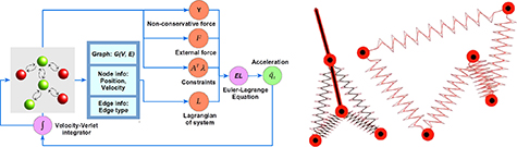
Figure 1. The LGnn framework. Visualization of a hybrid 2-pendulum-4-spring system and a 5-spring system.
Download figure:
Standard image High-resolution image2.2. Neural architecture of LGnn
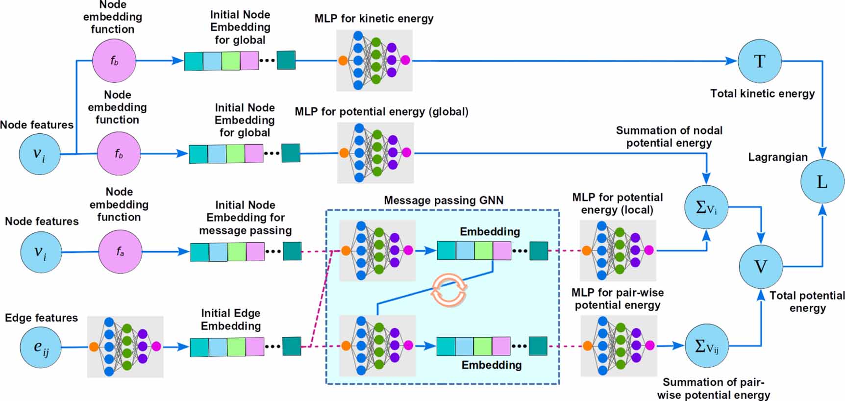
The neural architecture of LGnn is outlined in figure 2. The aim of the LGnn is to directly predict the Lagrangian of a physical system while accounting for its topological features. As such, the creation of a graph structure that corresponds to the physical system forms the most important step. To explain the idea better, we will use the running examples of two systems: (a) a double pendulum and (b) two balls connected by a spring, that represent two distinct cases of systems with rigid and deformable connections.
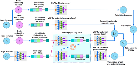
Figure 2. General architecture of Lagrangian graph neural network. Note that the drag predictions are similar to the kinetic energy computations. However, the drag is directly featured in EL equation and hence is not shown here.
Download figure:
Standard image High-resolution image2.2.1. Graph structure
The state of an n-body system is represented as a undirected graph,  , where nodes
  represents the particles,
  , and
, and  represents edges corresponding to constraints or interactions. In our running examples, the nodes correspond to the pendulum bobs and balls, respectively, and the edges correspond to the pendulum rods and springs, respectively. Note that the edges of the graphs may be predefined as in the case of a pendulum or spring system. The edges may also be defined as a function of the distance between two nodes such as
  where
where  is a distance function over node positions and θ is a distance threshold. This allows a dynamically changing edge set based on a cutoff distance as in the case of a realistic breakable spring.
2.2.2. Input features
Each node  is characterized by its type ti
, position
is characterized by its type ti
, position  , and particle velocity (
 ). The type ti
is a discrete variable and is useful in distinguishing particles of different characteristics within a system (Ex. two different types of balls). For each edge eij
, we store an edge weight
). The type ti
is a discrete variable and is useful in distinguishing particles of different characteristics within a system (Ex. two different types of balls). For each edge eij
, we store an edge weight  .
.
Finally, we note that the node input features are classified into two: global and local features. Global features are the ones that are not relevant to the topology and hence are not included in message passing. In contrast, local features are the ones that are involved in message passing. In our running example, while particle type is a local feature, particle position and velocity are global features.
2.2.3. Pre-processing
In the pre-processing layer, we construct a dense vector representation for each node ui
and edge eij
using  as:
as:


 is an activation function. As the acceleration of the particles is obtained using the EL equation, our architecture requires activation functions that are doubly-differentiable and hence,
  is an appropriate choice. In our implementation, we use different
  s for node representation corresponding to kinetic energy, potential energy, and drag. For brevity, we do not separately write the
  s in equation (3).
2.2.4. Kinetic energy and drag prediction
Since the graph uses Cartesian coordinates, the mass matrix is diagonal and the kinetic energy τi
of a particle depends only on the velocity  and mass mi
of the particle. Here, we learn the parameterized masses of each particle type based on the embedding
and mass mi
of the particle. Here, we learn the parameterized masses of each particle type based on the embedding  . Thus, the τi
of a particle is predicted as
. Thus, the τi
of a particle is predicted as  , where
  represent the concatenation operator, MLP
 represents an MLP for learning the kinetic energy function, and squareplus represents the activation function. The total kinetic energy of the system is computed as
  . The drag of a particle also typically depends linearly or quadratically to the velocity of the particle. Here, we compute the total drag of a system as
  . Note that while
  directly goes into the prediction of
  , ϒ is featured in the EL equation.
2.2.5. Potential energy prediction
In many cases, the potential energy of a system is closely dependent on the topology of the structure. To capture this information, we employ multiple layers of message-passing between the nodes and edges. In the lth layer of message passing, the node embedding is updated as:

where,  are the neighbors of ui
.
are the neighbors of ui
.  is a layer-specific learnable weight matrix.
  represents the embedding of incoming edge eij
on ui
in the lth layer, which is computed as follows.
represents the embedding of incoming edge eij
on ui
in the lth layer, which is computed as follows.

Similar to  ,
,  is a layer-specific learnable weight matrix specific to the edge set. The message passing is performed over L layers, where L is a hyper-parameter. The final node and edge representations in the Lth layer are denoted as
  and
and  respectively.
The total potential energy of an n-body system is represented as  , where vi
represents the energy of ui
due to its position and vij
represents the energy due to interaction eij
. In our running example, vi
represents the potential energy of a bob in the double pendulum due to its position in a gravitational field, while vij
represents the energy of the spring connected with two particles due to its expansion and contraction. In LGnn, vi
is predicted as
, where vi
represents the energy of ui
due to its position and vij
represents the energy due to interaction eij
. In our running example, vi
represents the potential energy of a bob in the double pendulum due to its position in a gravitational field, while vij
represents the energy of the spring connected with two particles due to its expansion and contraction. In LGnn, vi
is predicted as  . Pair-wise interaction energy vij
is predicted as
. Pair-wise interaction energy vij
is predicted as  . Although not used in the present case, sometime vi
can be a function of the local features dependent on the topology. For instance, in atomic systems, the charge of an atom can be dependent on neighboring atoms and hence the potential energy due to these charges can be considered as a combination of topology-dependent features along with the global features. In such cases, vi
is predicted as
. Although not used in the present case, sometime vi
can be a function of the local features dependent on the topology. For instance, in atomic systems, the charge of an atom can be dependent on neighboring atoms and hence the potential energy due to these charges can be considered as a combination of topology-dependent features along with the global features. In such cases, vi
is predicted as  , where
  represents the node MLP associated with the message-passing graph architecture.
2.2.6. Trajectory prediction and training
Based on the predicted  , and ϒ, the acceleration
  is computed using the EL equation (2). The loss function of LGnn is on the predicted and actual accelerations at timesteps
  in a trajectory
  , which is then back-propagated to train the MLPs. Specifically, the loss function is as follows.

Here,  is the predicted acceleration for the ith particle in trajectory
  at time t and
  is the true acceleration.
  denotes a trajectory from
  , the set of training trajectories. It is worth noting that the accelerations are computed directly from the position using the velocity-Verlet update and hence training on the accelerations is equivalent to training on the updated positions.
3. Experimental systems
3.1. n-Pendulum
In an n-pendulum system, n-point masses, representing the bobs, are connected by rigid bars which are not deformable. These bars, thus, impose a distance constraint between two point masses as

where, li
represents the length of the bar connecting the  th and ith mass. This constraint can be differentiated to write in the form of a Pfaffian constraint as

Note that such constraint can be obtained for each of the n masses considered to obtain the A(q).
The Lagrangian of this system has contributions from potential energy due to gravity and kinetic energy. Thus, the Lagrangian can be written as

where g represents the acceleration due to gravity in the y direction.
3.2. n-spring system
In this system, n-point masses are connected by elastic springs that deform linearly with extension or compression. Note that similar to a pendulum setup, each mass mi
is connected only to two masses  and
and  through springs so that all the masses form a closed connection. The Lagrangian of this system is given by

where r0 and k represent the undeformed length and the stiffness, respectively, of the spring.
3.3. Hybrid system
The hybrid system is a combination of the pendulum and spring system. In this system, a double pendulum is connected to two additional masses through four additional springs as shown in figure 1 with gravity in y direction. The constraints as present in the pendulum system are present in this system as well. The Lagrangian of this four-mass system is

where m1 and m2 represent masses in the double pendulum and m3 and m4 represent masses connected by the springs. Theorem 1.
theorem In the absence of an external field, LGnn exactly conserves the momentum of a system.
A detailed proof is given in supplementary material C. As shown empirically later, this momentum conservation in turn reduces the energy violation error in LGnn.
4. Implementation details
4.1. Dataset generation
4.1.1. Software packages
numpy-1.20.3, jax-0.2.24, jax-md-0.1.20, jaxlib-0.1.73, jraph-0.0.1.dev0
4.1.2. Hardware
Memory: 16GiB System memory, Processor: Intel(R) Core(TM) i7-10 750 H CPU @ 2.60GHz
All the datasets are generated using the known Lagrangian of the pendulum and spring systems, along with the constraints, as described in section 3. For each system, we create the training data by performing forward simulations with 100 random initial conditions. For the pendulum and hybrid systems, a timestep of 10−5 s is used to integrate the equations of motion, while for the spring system, a timestep of 10−3 s is used. The velocity-Verlet algorithm is used to integrate the equations of motion due to its ability to conserve the energy in long trajectory integration.
All 100 simulations for pendulum and spring system were generated with 100 datapoints per simulation. These datapoints were collected every 1000 and 100 timesteps for the pendulum and spring systems, respectively. Thus, each training trajectory of the spring and pendulum systems are 10 s and 1 s long, respectively. It should be noted that in contrast to the earlier approach, here, we do not train from the trajectory. Rather, we randomly sample different states from the training set to predict the acceleration. For simulating drag, the training data is generated for systems without drag and with linear drag given by  , for each particle.
4.2. Architecture
For Lnn, we follow a similar architecture suggested in the literature [6, 8]. Specifically, we use a fully connected feedforward neural network with two hidden layers each having 256 hidden units with a square-plus activation function. For LGnn, all the MLPs consist of two layers with five hidden units, respectively. Thus, LGnn has significantly lesser parameters than Lnn. The message passing in the LGnn was performed for two layers in the case of pendulum and one layer in the case of spring.
The kinetic energy term in Lnn is handled as in the earlier case where in the parametrized masses are learned as a diagonal matrix. In the case of LGnn, the masses are directly learned from the one-hot embedding of the nodes. Interestingly, we observe that the mass matrix exhibits a diagonal nature in LGnn without enforcing any conditions due to its topology-aware nature.
4.3. Training details
The training dataset is divided in 75:25 ratio randomly, where the 75% is used for training and 25% is used as the validation set. Further, the trained models are tested on its ability to predict the correct trajectory, a task it was not trained on. Specifically, the pendulum systems are tested for 10 s, that is 106 timesteps, and spring systems for 20 s, that is  timesteps on 100 different trajectories created from random initial conditions. All models are trained for 10 000 epochs with early stopping. A learning rate of 10−3 was used with the Adam optimizer for the training. The performance of both L1 and L2 loss functions were evaluated and L2 was chosen for the final model. The results of LGnn and Lnn with both the losses are provided in the supplementary material.
 Lagrangian graph neural network
| Parameter | Value |
|---|---|
| Node embedding dimension | 5 |
| Edge embedding dimension | 5 |
| Hidden layer neurons (MLP) | 5 |
| Number of hidden layers (MLP) | 2 |
| Activation function | Squareplus |
| Number of layers of message passing (pendulum) | 2 |
| Number of layers of message passing (spring) | 1 |
| Optimizer | ADAM |
| Learning rate |

|
| Batch size | 100 |
 Lagrangian neural network
| Parameter | Value |
|---|---|
| Hidden layer neurons (MLP) | 256 |
| Number of hidden layers (MLP) | 2 |
| Activation function | Squareplus |
| Optimizer | ADAM |
| Learning rate |

|
| Batch size | 100 |
-
Trajectory visualization For visualization of trajectories of actual and trained models, videos are provided as supplementary material. The GitHub link https://github.com/M3RG-IITD/LGNN contains:
- (a)Hybrid system: double pendulum and two masses connected with four springs under gravitational force as shown in figure 1.
- (b)Hybrid system with external force: double pendulum and two masses connected with four springs under gravitational force as shown in figure 1. A force of 10 N in x-direction is applied on the second bob of double pendulum.
- (c)Five spring system: five balls connected with five springs as shown in figure 1.
5. Empirical evaluations
In this section, we evaluate LGnn and establish that, (a) LGnn is more accurate than Lnn in modeling physical systems, and (b) owing to topology-aware inductive modeling, LGnn generalizes to unseen systems, hybrid systems with no deterioration in efficacy for increasing system sizes.
5.1. LGnn for n-pendulum and n-spring systems
In order to evaluate the performance of LGnn, we first consider two standard systems, that have been widely studied in the literature, namely, n-pendulum and n-spring systems [4, 6, 8, 9], with  . Following the work of [8], we evaluate performance by computing the relative error in (a) the trajectory, known as the rollout error, given by
  and (b) energy violation error given by
  ). The training data is generated for systems without drag and with linear drag given by
  , for each particle. The timestep used for the forward simulation of the pendulum system is 10−5 s with the data collected every 1000 timesteps and for the spring system is 10−3 s with the data collected every 100 timesteps. The details of the experimental systems, data-generation procedure, the hyperparameters and training procedures are provided in the Methods section.
LGnn is compared with (a) Lnn in Cartesian coordinates with constraints as proposed by [8], which gives the state-of-the-art performance. Since, Cartesian coordinates are used, the parameterized masses are learned as a diagonal matrix as performed in [8]. In addition, LGnn is also compared with two other graph-based approaches suggested in [5, 6], named as (b) Lagrangian graph network (Lgn), and (c) Graph network simulator (Gns). Lgn exploits a graph architecture to predict the Lagrangian of the physical system, which is then used in the EL equation. Gns uses the position and velocity of the particles to directly predict their updates for a future timestep [4]. For both these approaches, since no details of the exact architecture is provided [5, 6], a full graph network is employed [16]. All the simulations and training were performed in the JAX environment [18]. The graph architecture of LGnn was developed using the jraph package [19]. All the codes related to dataset generation and training are available at https://github.com/M3RG-IITD/LGNN.
Figure 3 shows the energy violation and rollout error of LGnn and Lnn for pendulum and spring systems with 3, 4, and 5 links without drag on each of the particles. For the pendulum system, LGnn is trained on 3-pendulum and for spring, LGnn is trained on 5-spring systems. The trained LGnn is used to perform the forward simulation on the other unseen systems. In contrast, the Lnns are trained and tested on the same systems. We observe that the LGnn exhibits comparable rollout error with Lnn for pendulum system, even on unseen systems. Further, LGnn exhibits significantly lower rollout error for spring systems—where the topology plays a crucial role—giving superior performance than Lnns consistently. Due to the chaotic nature of these systems, it is expected that the rollout error diverges. However, energy violation error gives a better evaluation of the realistic nature of the predicted trajectory. Interestingly, we note that the energy violation error is fairly constant for LGnn for both pendulum and spring systems. Moreover, the error on both seen and unseen systems are comparable suggesting a high degree of generalizability for LGnn. The geometric mean of energy violation error and rollout error of Lnn and LGnn for systems with and without drag are provided in the Supplementary material.
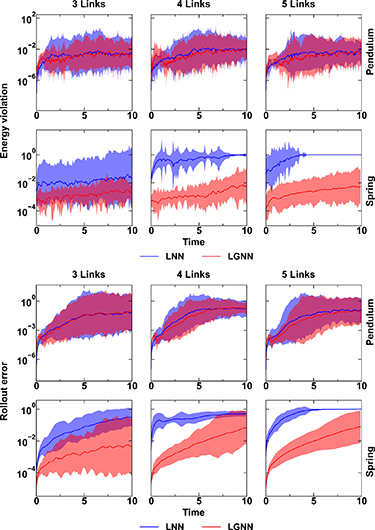
Figure 3. Energy violation (left) and rollout error (right) of LGnn (red) and Lnn (blue) for pendulum and spring systems having 3, 4, and 5 links and subjected to linear drag. Note that the LGnns for pendulum and springs are trained on 3 and 5 links, respectively, and tested on all the systems. Lnns are trained and tested separately on each of the systems. Shaded region shows the 95% confidence interval from 100 initial conditions.
Download figure:
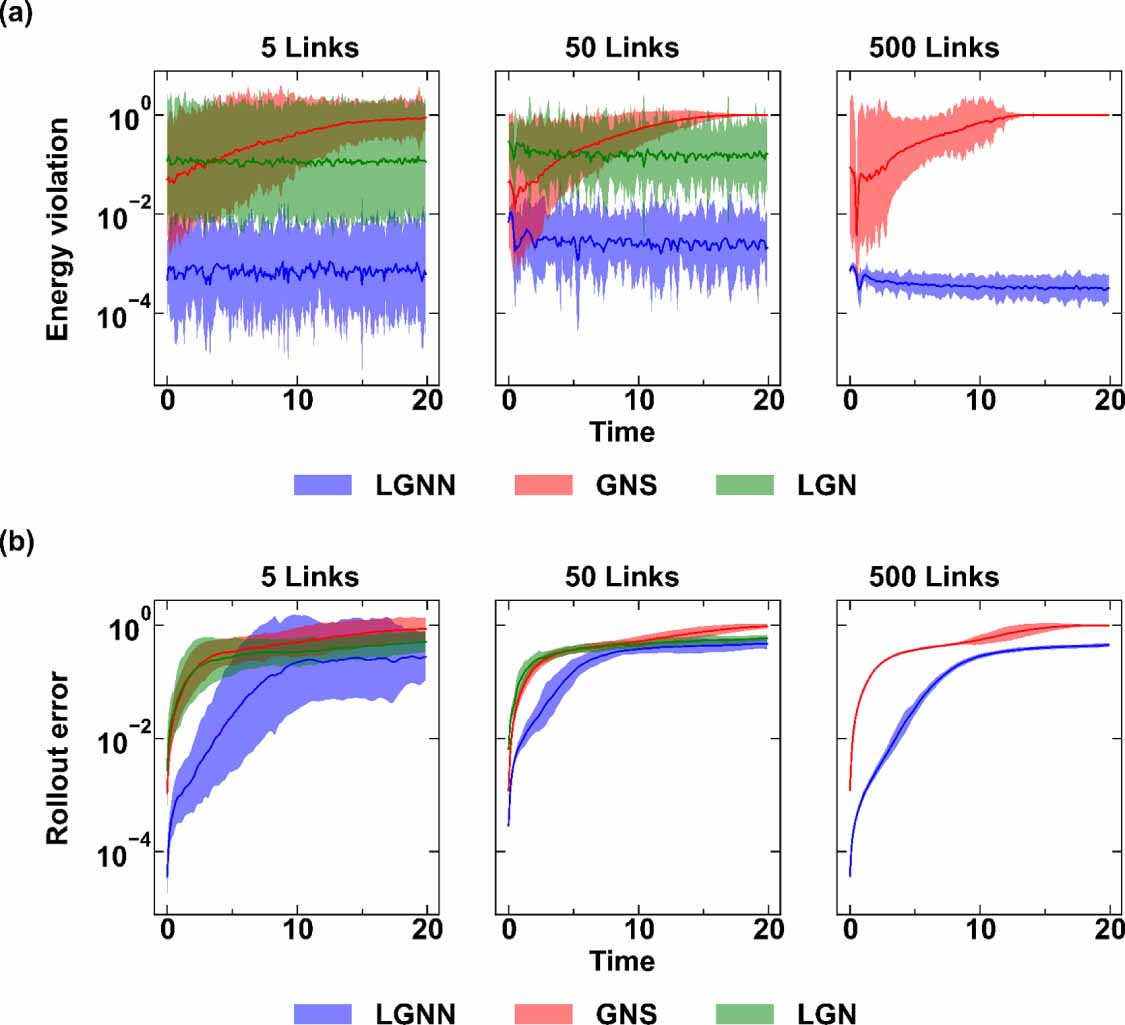
Standard image High-resolution image5.2. Generalizability
Now, we examine the ability of LGnn to push the limits of the current approaches. A regular Lnn uses a feed-forward NN to take the entire  as the input and then predicts the Lagrangian. Owing to this design, the number of model parameters grows with the input size. Hence, an Lnn trained on an n-sized system cannot be applied for inference on an nʹ-sized system, where
  . This makes Lnn
transductive in nature. In contrast, LGnn is inductive, wherein the parameter space remains constant with system size. This is a natural consequence of our design where the learning happens at node and edge levels. Hence, given an arbitrary-sized system, we only need to predict the potential and kinetic energies at each node and edge, which we then aggregate to predict the combined energies at a system level. Further, a complex system that is unseen, if divisible into multiple sub-graphs with each sub-graph representing a learned system, the overall system can be simulated with zero-shot generalizability.
. This makes Lnn
transductive in nature. In contrast, LGnn is inductive, wherein the parameter space remains constant with system size. This is a natural consequence of our design where the learning happens at node and edge levels. Hence, given an arbitrary-sized system, we only need to predict the potential and kinetic energies at each node and edge, which we then aggregate to predict the combined energies at a system level. Further, a complex system that is unseen, if divisible into multiple sub-graphs with each sub-graph representing a learned system, the overall system can be simulated with zero-shot generalizability.
Figure 4 shows the energy and rollout error of spring systems with 5, 50, 500 links using LGnn, Lgn and Gns trained on 5-spring system. We observe that LGnn performs significantly better than the other baselines. Note that the results of Lgn for 500 springs are not included due to significantly increased computational time for the forward simulation in comparison to the other models. In addition to the rollout error, we observe that the energy violation error of LGnn remains constant with low values even for systems that are two orders of magnitude larger than the training set. This suggests that the LGnn can produce realistic trajectories on large scale systems when trained on much smaller systems. These results also establish the superior nature of LGnn architecture, which exhibits improved performance with higher computational efficiency. The performance of similar systems with drag is provided in the supplementary material.

Figure 4. (a) Energy violation and (b) rollout error for 5, 50, and 500 spring system with LGnn trained on 5 spring system. Shaded region shows the 95% confidence interval from 100 initial conditions.
Download figure:
Standard image High-resolution imageTo test generalizability to an unseen system, we consider a hybrid system with 2-pendulum-4-springs as shown in figure 1. The LGnns trained on the 5-spring and 3-pendulum systems are used to model the hybrid system. Specifically, the  of the physical system is considered as the union of the
  of two subgraphs, one representing the pendulum system and the other representing the spring systems. Then, the computed
  is substituted in the EL equation to simulate the forward trajectory. Figures 5(a) and (b) shows the energy violation and rollout error on the hybrid system. We observe that both these errors are quite low and are not growing with time. This suggests that LGnn, when trained individually on several subsystems, can be combined to form a powerful graph-based simulator. Videos of simulated trajectories under different conditions, such as external force, are provided at https://github.com/M3RG-IITD/LGNN for visualization.

Figure 5. (a) Energy violation and (b) rollout error of LGnn in the unseen hybrid system. (c) Learned node-level drag force. (d) Data efficiency of Lnn and LGnn on 3-spring system.
Download figure:
Standard image High-resolution image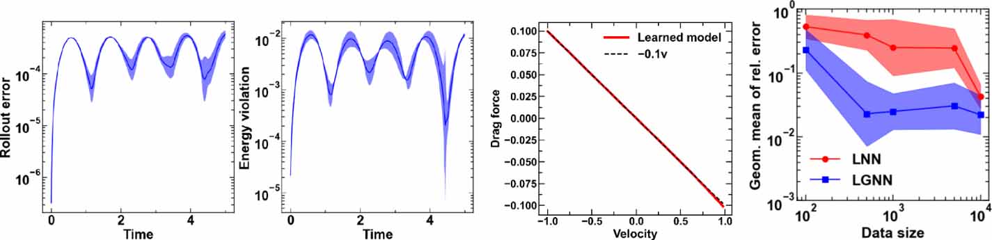
5.3. Interpretability and data efficiency
The trained LGnn provides interpretability, thanks to the graph structure. That is, since the computations of LGnn are carried out at the node and edge levels, the functions learned at these level can be used to gain insight into the behavior of the system. Further, the parameterized masses of the systems are learned directly during the training of LGnn, leading to a diagonal mass matrix. This is in contrast to Lnn where the prior information that mass matrix remains diagonal in the Cartesian coordinates is imposed to make the learning simpler [8].
Figure 5(c) shows the learned drag force as a function of velocity. We observe that the neural network has learned the drag in excellent agreement with the ground truth. Thus, in cases of systems where the ground truth is unknown, the learned drag can provide insights into the nature of dissipative forces in the system. Similarly, the λ learned during the training directly provides insights into the magnitude of the constraint forces.
Finally, we analyze the efficiency of LGnn to learn from the training data. To this extent, we train both models on a 3-spring system with (100, 500, 1000, 5000, 10 000) datapoints. Figure 5(d) shows the geometric mean of relative error on the trajectory of the system. We observe that LGnn consistently outperforms Lnn, Further, the performance of LGnn saturates with 500 datapoints. In addition, LGnn trained on these 500 datapoints exhibits ∼25 and ∼3 times better performance in terms of geometric relative error than Lnn trained on 500 and 10000 datapoints. This confirms that the topology-aware LGnn can learn efficiently from small amounts of data, still yield better performance than Lnn.
6. Conclusions and outlook
Altogether, we demonstrate a novel graph architecture, namely LGnn, which can learn the dynamics of systems directly from the trajectory, while exhibiting superior energy and momentum conservation. We show that the LGnn can generalize to any system size ranging orders of magnitude, when learned on a small system. Further, LGnn can even simulate unseen hybrid systems when trained on the systems independently. Finally, we also show that LGnn exhibits better data-efficiency, learning from smaller amounts of data in comparison to the original Lnn.
There are several future directions that the present work opens up. The LGnn, at present, is limited to systems without collisions and other deformations. Extending LGnn to handle elastic and plastic deformations in addition to collisions can significantly widen the application areas. Further, LGnn assumes the knowledge of constraints. Automating the learning of the constraints while training the model using neural networks can provide a new paradigm to learn the constraints along with the Lagrangian. The graph nature of LGnn can potentially supplement the learning of constraints. Although, the message passing in LGnn is translationally and rotationally invariant, the expressive power is limited as only the distance is given as the edge feature. Enhancing the feature representation, and message passing through architectural modifications as in the case of equivariant Gnns can increase the applicability to more complex applications such as atomistic simulations of materials.
Data availability statement
All data that support the findings of this study are included within the article (and any supplementary files).
Data and code availability
All the codes related to dataset generation and training are made are available at https://github.com/M3RG-IITD/LGNN.
Conflict of interest
Authors declare no competing interests.
Supplementary data (0.4 MB PDF)