
Abstract
In order to guarantee machining quality and production efficiency and as well as to reduce downtime and cost, it is essential to receive information about the cutting tool condition and change it in time if necessary. To this end, tool condition monitoring systems are of great significance. Based on the data fusion technology of multi-sensor integration and the learning ability of deep residual network, a tool wear monitoring system is proposed in this paper. For data acquisition, multiple sensors are used to collect vibration, noise and acoustic emission signals in the machining process. For signal processing, the data fusion method of angular summation of matrices is used, so that the multi-source data are fused into two-dimensional pictures. Then, the feature extraction module of the proposed system uses the pictures as input and takes advantage of the deep residual convolutional network in extracting the deep features from the pictures, and finally the identification module completes the recognition of the tool wear type. To verify its feasibility, a testing bed is built on a CNC milling machine, and multi-sensor data are collected during the machining process of a simple workpiece with one of the two selected cutting tools each time. The proposed system is trained using the collected data and then is used to monitor the wear condition of a new cutting tool by collecting real-time data under similar condition. The results show that the accuracy of wear state recognition is as high as 90%, which verifies the feasibility of the proposed tool wear monitoring system.
Export citation and abstract BibTeX RIS
1. Introduction
Tool condition monitoring (TCM) is of vital importance to modern manufacturing systems. With a TCM system, it is possible in machining to obtain in real time the wear condition information of the cutting tools and then automatically modify the cutting parameters, so as to optimize the machining process. According to statistics, TCM systems would reduce the downtime of computer numerical control (CNC) machine tools by 75% and improve their productivity by 10%-60%.TCM systems also greatly improve the utilization rate of the cutting tools and save more than 30% of the processing time and production cost [1].
To monitor the tool condition online, data-driven methods are generally preferred and adopted with various sensors. Dimla and Lister [2] developed an online tool wear condition monitoring system for turning. They used a prop dynamometer to measure the components of the cutting force in three directions mutually perpendicular to each other. Tool wear condition was identified through signal time series and fast Fourier transform (FFT) analysis. Salgado et al [3] took advantage of the feed motor current and sound signal, and used the least squares support vector machine (LS-SVM) to estimate the feed cutting force, and then used the singular spectrum analysis (SSA) to extract the internal information related to tool wear from the sound signal. Research by Ghosh et al [4] showed that the tool condition monitoring results obtained by using sensors for the current of the motor spindle are quite close to the results achieved by using cutting force sensors. Alonso and Algado [5]developed a tool wear condition monitoring system (TCMS) that used vibration signals to detectthe wear. In terms of multi-sensor fusion, Kai Feng Zhang et al [6] proposed a TCM method that integrated acoustic emission (AE) signals with acoustic signals during cutting. Each signal was filtered by time-frequency method based on multifractal theory, and features were extracted. Support vector machine (SVM) integration model was used to realize the decision-making level fusion of information. Xie et al [7] presented a TCM method using an innovative tool holder with multi-sensor integration, which can wirelessly measure three-axis components of the cutting force, torque and cutting vibration simultaneously in milling operations. Paul and Varadarajan [8] combine sensor signals such as cutting force, cutting temperature and tool vibration to predict tool wear in turning AISI 4340 steel. Wu et al [9] used a fuzzy reasoning system to determine the remaining tool life taking advantage of the sensor fusion methods (including acoustic emission, vibration and electrical current sensors). C. Aliustaoglu et al [10] used sensor fusion model to identify tool wear based on sound, force and vibration signals with the help of fuzzy reasoning system.
In recent years, the powerful performance of deep learning methods has been demonstrated in many disciplines as well as in tool condition monitoring. Qiao et al [11] proposed a model named TDConvLSTM, which was a convolutional recurrent network based on temporal distribution. The sensor signals of temporal input were simultaneously applied to each sub-sequence for local feature extractors of temporal distribution to extract local spatio-temporal features, and tool wear was predicted by a fully connected layer stacked on top of the model. An et al [12] extracted the time-domain features of the sensor data through one-dimensional convolutional neural network CNN, and then used the powerful temporal memory ability of long short-term memory network LSTM to predict the remaining service life of the tool. Yu et al [13, 14] conducted in-depth analysis of time series classification and mechanical state monitoring with recurrent neural network (RNN) autoencoder, and demonstrated reasonable performance in the estimation of the remaining service life of machinery. In order for better practicability, Sonali et al [15] designed an artificial neural network(ANN) classifier based on statistical learning of machining vibration, and concluded that the ANN model based on deep learning led to more accurate results in monitoring tool wear condition as compared with machine learning classifiers. Mukherjee and Das [16] used artificial neural network as a data analysis tool and back-propagation algorithm as a learning algorithm to design a system that could effectively monitor tool state online. Zeng et al [17] Proposed a tool monitoring model based on multi-source sensor data fusion and attention mechanism, and preliminarily verified the main algorithms using open data sets. Based on previous work, this paper aims to present a practical approach to tool wear condition monitoring in CNC milling process. The main contributions of this work are summarized as follows:
- (a)A new tool wear condition monitoring system is designed, and its feasibility is demonstrated in the testing experiment.
- (b)The system adopts the new fusion technology of multi-sensor information on the data layer, and combines it with the deep learning method of deep residual network to extract the data features, which makes it more effective in tool wear prediction in actual machining.
The rest of this paper is organized as follows: the second part introduces the design and implementation issues of the tool wear monitoring system. The third part describes the construction of the testing platform and the cutting experiment for data collection. The fourth part deals with the training and verification of the system.
2. The proposed TCM system
2.1. Overall structure
In this paper a tool wear condition monitoring system is proposed based on multi-sensor integration and deep residual convolution network. The proposed tool wear monitoring system is designed as part of an online tool wear management system attached to the CNC machine. It is supposed to collect indirect data about tool wear during the machining process, identify the tool condition and report to the controller for tool management. Because the cutting tools are difficult to measure directly in machining, a combination of sensors are used to collect multi-source data related to the cutting, and deep learning methods are employed to estimate the tool condition indirectly.
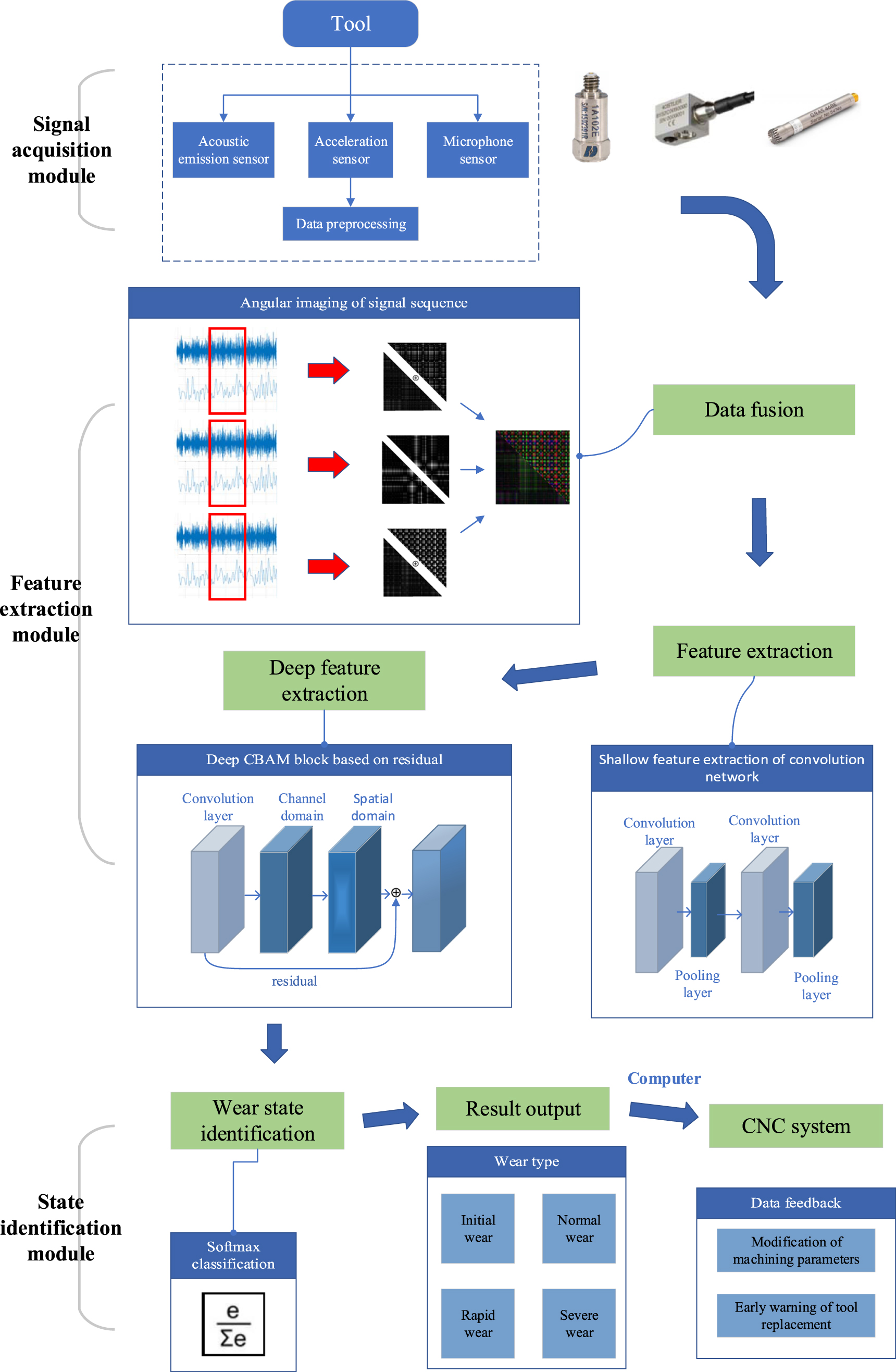
Figure 1 shows the framework of the proposed tool wear monitoring system. It is mainly comprised of three functional modules namely signal acquisition, feature extraction, and tool condition identification.
- (1)The signal acquisition module. This module is for data collection and preprocessing. In order to minimize the interference in the collected data, a number of sensors are employed and multiple sets of data from the same sensor are used. Combined data sets may reduce the system's sensitivity to noise and temporary faults. Multiple independent sensor data sources help improve accuracy by eliminating ambiguities in the data. In this system, multi-sensor fusion technology is adopted for data acquisition. The multi-sensor signals complement each other in tool wear perception, with the advantages of strong anti-interference ability and wide coverage of information. In order to ensure the multi-source data collected during machining carry effective information about the cutting tool condition, a selection of sensors (acoustic emission sensors, sound sensors and acceleration sensors in this case) should be installed near the cutting area systematically. The data signals collected by the multi-sensors will be amplified first, with the initial and final signal segments being cut out, then transferred to the database to form the initial data. This makes it convenient for the feature extraction module to perform the subsequent data processing and analysis tasks.
- (2)Feature extraction module. This module is the main part of the system in terms of computation and machine learning. It is responsible for two important tasks: signal data fusion imaging and feature extraction. In order to comprehensively analyze the condition of cutting tools, angular matrix imaging of signal sequence is used to map the collected multi-sensor signals into two-dimensional images containing time series features, and the signals are transformed into image input forms that are easier to be recognized and processed by the deep learning module, which will be discussed in detail in section 2.2. The second task is feature extraction. It uses the obtained images first as input for two-layer convolution network to extract shallow features, and then as input for deep residual network to extract deep features of the data through deep learning. For better extraction, the deep residual network takes the advantage of attention mechanism by combining with a Convolutional Block Attention Module (CBAM). Specifically, CBAM block is formed by serial connection of channel attention mechanism module unit and spatial attention mechanism module. On this basis, the residual unit connects the CBAM input and output through layer hopping connection, which will be discussed in detail in section 2.3. The application of attention mechanism is CBAM block of comprehensive channel and spatial domain, which will be addressed in detail in sections 2.2 and 2.3.
- (3)Tool wear state identification module. The main function of this module is to determine the wear state of the tool. Since the output of the feature extraction module is not yet the desired final decision, it is necessary to combine the high-dimensional features extracted from the previous deep residual network with local important features, and send the final feature vector to the Softmax classifier through global pooling, so as to realize the mapping of data features and sample labels, and then realize the classification of tool wear states. At the same time, the classification results are stored in the tool management database of the computer, and the CNC system can obtain corresponding feedback instructions according to the classification results. For example, when the tool is detected to be in the rapid wear state, the cutting parameters may be changed to extend the tool life or a warning be issued in advance. When the tool is detected to be in the severe wear state, the tool replacement warning will be issued or start a tool change operation.
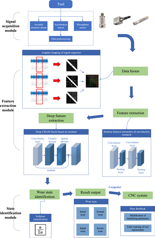
Figure 1. Structure of the tool wear monitoring system.
Download figure:
Standard image High-resolution image2.2. Angular matrix imaging of signal sequences
The angular matrix imaging method reported in the literature [18] is utilized in this paper to fuse sensor signals of multiple dimensions at the data level. Taking for example the signal imaging measured by piezoelectric acceleration sensor, the collected signal is a point set of  where
where  represents the acceleration value measured at the corresponding time point (obtained by signal amplifier), and
  represents the timestamp. Assume
  is the polar coordinates for each point
  After standardizing the acceleration value at the
  time point and then the angle
  in the form of corresponding polar coordinate representation is obtained as arccosine of the normalized value of
  and
and  is obtained by reducing the
  unit. By doing this in turn for all the signal points on the time axis, the polar coordinate transformation of a sensor signal is completed. After transforming the scaled time series into polar coordinates, the time relationship between different time points is identified by calculating the cosine value of each time point. The specific imaging process is shown in table 1.
Table 1. Angular matrix imaging process.
| S. no. | The content of process |
|---|---|
| 1. | • The signal time series  ={ ={
 ..., ...,  ..., ...,  } is normalized and reduced to the value } is normalized and reduced to the value  of of  at each time point, resulting in at each time point, resulting in  ={ ={
 ..., ...,  ..., ...,  }, where }, where  Each Each  is reduced by unit to get is reduced by unit to get  where where  and and  is the regularization factor, and the polar coordinate transformation is completed. is the regularization factor, and the polar coordinate transformation is completed. |
| 2. | • For each element of  the corresponding the corresponding  is calculated as is calculated as  则 则
|
| 3. | • Note 
|
| 4. | • Let  make Kronecker products with their transpose matrices respectively, and then make the difference to get a symmetric matrix make Kronecker products with their transpose matrices respectively, and then make the difference to get a symmetric matrix  which contains the time information in the data which contains the time information in the data |
| 5. | • All elements of the lower triangle of matrix  are set to 0 to obtain the upper triangle matrix are set to 0 to obtain the upper triangle matrix  that is, the two-dimensional matrixization of the signal data of a single sensor is completed. that is, the two-dimensional matrixization of the signal data of a single sensor is completed. |
| 6. | • Repeat Step1-Step5 operation to obtain  for another sensor signal collected, and transpose for another sensor signal collected, and transpose  to obtain matrix to obtain matrix  By adding By adding  the two-dimensional matrix containing two sensor data is completed, and one channel image is obtained. the two-dimensional matrix containing two sensor data is completed, and one channel image is obtained. |
Following these steps, the multi-sensor data are prepared in pairwise combinations to form two-dimensional matrices by means of imaging, these data are then wrapped as one channel image. When there are three single-channel images, they can be combined into an RGB three-channel image as the data input of the subsequent module. Based on this method, the inherent time relationship of each sensor signal can be retained to achieve effective integration of sensor data in data layer. The visual effect of sensor data fusion is intuitively displayed by feature pictures.
2.3. Deep residual network based on attention mechanism
The essence of the attention mechanism is to focus on useful information and avoid interference. By automatically adjusting the parameter configuration after system training, it can extract useful information like human vision, reduce the interference of useless information, and improve the extraction efficiency. In this paper, the attention mechanism functions by means of a channel attention unit and a spatial attention unit together, which are combined in order in every block. Since the attention mechanism starts in two dimensions, which can complement each other, making the network pay attention to important features and suppress unnecessary ones. In order to increase the ability to mine deep features from the data, a residual block structure is added on the basis of attention mechanism, which forms an attention-based residual unit. The depth of the network may be improved by increasing the number of this unit the residual unit within the network.
Figure 2 shows the structure of a single attention-based residual unit.  represents the feature map obtained by the convolution operation of the previous residual unit based on attention mechanism, it can be seen that feature map F has three-dimensional features, and H, W and C represent the size in three directions respectively;
  represents the feature map after channel attention extraction;
  represents the feature map after spatial attention extraction;
  represents the operation of attention extraction in the channel dimension;
  represents the operation of attention extraction in the spatial dimension.

Figure 2. Residual unit based on attention mechanism.
Download figure:
Standard image High-resolution imageAs shown in figure 2, the channel attention mechanism works as follows: the feature map  is taken with dimension
  as input, and then go through global maximum pooling and global average pooling based on width and height to obtain two feature maps. Next, they are sent to a two-layer artificial neural network (MLP) respectively, and the features output by MLP are added based on element summation. After sigmoid activation, the final channel attention feature is generated, that is,
  Finally, perform element-wise multiplication between
  and input feature map
  to generate input feature
  required by spatial attention module.
The spatial attention mechanism is realized as follows: the feature map  outputted from the channel attention module is used as the input feature map. First, do a global maximum pooling and a global average pooling based on channel to get two
  feature maps, and then do channel splicing based on channel dimension. After that, through a 7* 7 convolution operation, the dimension is reduced to one
  single-channel feature map. And then the sigmoid function generates a spatial attention feature
  Finally, the feature is multiplied with the input feature
  of the module to obtain the final feature
3. Cutting experiment and data collection
3.1. Testing platform
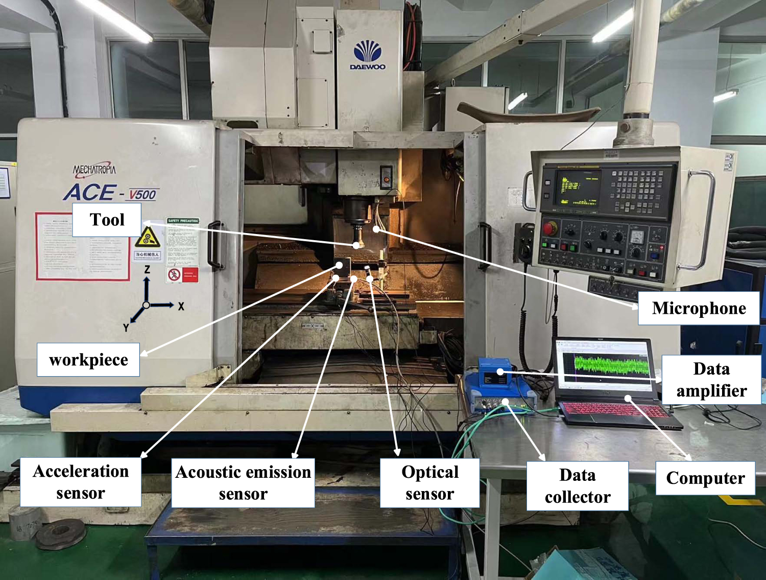
As mentioned above, the proposed multi-sensor TCM system is supposed to work with CNC milling machine tools. Major parameters of the CNC machine tool related to the machining test are shown in table 2. To collect tool condition data and train the system, the ACE-V500 vertical machining center is utilized, with sensors including an acceleration sensor, acoustic emission sensor and microphone sensor mounted as shown in figure 3. The workpiece is a hexahedral block (200 mm * 100 mm * 60 mm) made of 45#steel (GB/T699-1999). A high-speed data collector (TranAX 4.1) is selected for data acquisition in the experiment. The sampling frequency is set to 10 kHz for the experiment.
Table 2. Major parameters of the machine tool.
| Main technical parameters | Parameter value or range |
|---|---|
| Spindle speed range | 80 ∼ 10000 r min−1 |
| Feed speed | 1 ∼ 8000 mm min−1 |
| Positioning accuracy | ±0.005 mm |
| Repeat positioning accuracy | ±0.002 mm |
| Area of work table | 1200 × 500 mm |
| Stroke of each coordinate axis (x, y, z) | X: 0∼−1020 mm |
| Y: 0∼−500 mm | |
| Z: 0∼−510 mm | |
| Tool magazine capacity | 30 |
| Tool replacement time | 1.5 s |
| Spindle interface taper | BT40 |
| Numerical control system | FANUC 18M |

Figure 3. Testing platform for the tool wear monitoring system.
Download figure:
Standard image High-resolution imageIt is worth mentioning that the indirect method of measurement is more economical and practical for online monitoring of tool conditions, as long as the sensors used in a TCM system fit in well with the whole machining system. At present, the commonly used sensor signals include cutting force, acceleration, acoustic emission, current and sound. Among them, the cutting force signal has higher sensitivity and faster response, but the installation of a dynamometer often requires retrofitting of the machine tool. Balance the accuracy, cost, and installation, the acceleration sensor, acoustic emission sensor and microphone sensor are selected for data collection purpose in this paper. Table 3 lists the detailed information of the selected sensors. In addition, an MV-CE060-10UM optical sensor is used in the experiment for measurement of the tool wear.
Table 3. Sensors selected in the experiment.
| Sensor | Model | Measurement direction | Sensitivity | Frequency range |
|---|---|---|---|---|
| X: 11.08 | ||||
| Y: 10.5 | ||||
| Acceleration sensor | 1A102E | X, Y, Z | X: 11.08 Y: 10.5 Z: 10.91 (mV/g) | 1 ~ 10 kHz |
| Acoustic emission sensor | 8152C1 | one-way | 48 (V/(m/s)) | 100 ~ 900 kHz |
| Microphone sensor | GRAS 46BE | one-way | 3.6 (3.6 mV Pa−1) | 4 ~ 80 kHz |
The sensors for indirect measurement of the cutting tool are mainly positioned on the workpiece, spindle, fixture or workbench. The closer they are to the cutting area in the actual data acquisition process, the higher the signal intensity and quality of the collected data. Therefore, in this paper, the acceleration sensor is attached to the workpiece with strong glue. In addition, considering that the material to be processed in this experiment is non-magnetic, the AE sensor with magnetic holder is arranged on the fixture close to the cutting area. The signal from the microphone sensor is transmitted through sound waves. In order to collect the highest quality sound signal, the microphone sensor is placed close to the cutting area.
3.2. Measurement and state classification of tool wear
Before application of the proposed system, it is necessary to collect data and use them to train the network for wear state recognition in machining. To that end, cutting experiments are carried out following a number of steps.
Step 1: Install a new cutting tool and set up the workpiece. The tool is made of cemented carbide, with MT-TiCN + Al2O3 coating.
Step 2: Calibrate the microphone sensor for data acquisition, with its sampling frequency set to 10 kHz.
Step 3: Install acceleration and acoustic emission sensors on the surface of the workpiece, and install the microphone sensor as close as possible to the cutting tool.
Step 4: Set machining parameters are set according to table 4.
Table 4. Machining parameters for the cutting experiment.
| Spindle speed (rpm) | Axial cutting depth (mm) | Cutting width (mm) | Feed rate (mm/min) | Lubrication method | Cutting mode |
|---|---|---|---|---|---|
| 400 | 0.2 | 60 | 50 | Dry cutting | Down milling |
Step 5: Start cutting the workpiece and the signals are acquired during the period from the moment when the cutting tool cuts in the workpiece to the end of the cutting. After each cutting operation, the spindle of the machine tool is assigned to a fixed starting position, and then adjust the rotation angle of the cutter holder and use the optical sensor to take high-definition pictures of the rear face of cutter, and record the wear amount of the tool.
Repeat step 5 until the tool is worn out. In actual cutting, when the wear amount on the rear face of the cutter reaches 0.2 mm, the cutter is replaced. The complete life of such a tool is recorded, and then another tool is used for cutting. In this way, two tools are measured, and the data obtained are recorded as T1 and T2 respectively for later use.
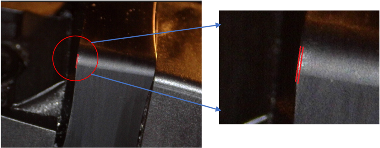
For the measurement method of tool wear in step 5, the following values are mentioned: if the tool is removed at the end of each cutting cycle and the wear value is measured manually, this method is too time-consuming and does not guarantee the continuity of the experiment. Therefore, we improve this method. At the beginning of the cutting cycle, that is two or three times cutting cycle, the optical sensor takes the high-definition picture of the back of the tool and takes the tool out. The wear of the back of the tool in the high-definition picture is taken as the measurement standard, i.e. the 1 mm standard, and then the actual wear is measured with the microscope, i.e. the standard value. As shown in figure 4, by setting the light angle, the brightness of the wear area on the back of the tool becomes more pronounced. By measuring the width of the gap between the two red lines marked in the photograph and multiplying by the standard, the actual wear amount can be obtained. In this way, the actual wear value of the tool can be obtained for all the cutting cycles.

Figure 4. Schematic diagram of the wear measurement method.
Download figure:
Standard image High-resolution image4. Training and verification
4.1. Data preprocessing and system training
As pointed in the literature [19], tool wear roughly follows a certain pattern, from initial wear through normal wear to severe wear. In the normal wear stage, the rough surface of the cutting edge is worn off, the working pressure becomes even, and the tool wear is relatively slow. The cutting tool works effectively in this stage. Then, the friction and cutting temperature between the tool and the workpiece would increase, and consequently, the tool wear would speed up significantly. After that, the tool condition gradually evolves into severe wear condition, under which the tool is unable to guarantee actual machining requirements and would even lead to tool crack or machine halt. Therefore, the TCM system needs to effectively identify the tool condition before it enters the severe wear state.
Figure 5 shows the wear curves in full lifecycle of the cutting tools (T1 and T2), which are obtained based on the wear amounts measured during the cutting experiment. It shows that the wear amount increases quickly in the initial wear stage, which lasts only a short time, then the wear develops steadily until it approaching 0.02 mm, and finally the tool is worn out and changed after about 64 consecutive cutting cycles. As the cutting tools in severe wear condition are prone to cause severe problems and the tool condition usually degenerate quickly just before it enters the severe wear state, a rapid wear state is inserted, in order for quick recognition of the tool condition before in enters the severe state. Thus, the tool wear process is divided into four states: initial wear, normal wear, rapid wear and severe wear. Figure 6 shows the worn rear face of a cutting tool (T1) measured in different wear states during the experiment.

Figure 5. Wear curve of the cutting tools used in the experiment.
Download figure:
Standard image High-resolution image
Figure 6. Different wear states of the cutting tool.
Download figure:
Standard image High-resolution imageIt is worth noting that the time series of each cutting sample collected is up to 200 000. In order to reduce the adverse effect of class imbalance on the performance of feature extraction module, under-sampling methods are also used to balance the data between the wear types, as indicated in table 5.
Table 5. Division of under sampled data.
| Wear type | Initial wear | Normal wear | Rapid wear | Severe wear |
|---|---|---|---|---|
| Cutting cycles | 1–6 | 7–53 | 54–60 | 61–64 |
| Data segments per sample | 8 | 1 | 7 | 12 |
| Data volume | 48 | 47 | 49 | 48 |
| Data amount ratio | 1 | 0.98 | 1.02 | 1 |
After data collection and data preprocessing, the TCM system is trained using the collected data. In order for stable signal processing and feature extraction, certain computer hardware is used including a Core i7700 processor with the clock frequency of 3.6 GHz, a DDR4 64GB memory and a GeForce RTX 2080ti GPU. The software adopts a deep learning framework with Keras as the front-end and Tensorflow as the back-end.
Hyperparameters also play an important role in guaranteeing the performance of the deep learning model. In this work, the grid search method is adopted to preliminarily select the hyperparameters for deep learning model. Based on previous work [17], the Learning rate, Epoch, and Batch Size are respectively set to 0.001, 100 and 32; and the optimizer works in Adam mode. Authors are referred to reference [20] for detailed illustration on hyperparameters selection.
4.2. Testing experiment and results analysis
In order to verify the trained monitoring system, a cutting experiment under similar cutting conditions with a new cutting tool (T3) is conducted. The same sensors are used to collect real-time signals for the trained system to recognize the tool wear state. As in the data-collection experiment, the cutting involves quite a number of cycles, but it does not need to stop for measurement after each cycle. The cutting is supposed to continue until the monitoring system reports a sever state. However, in order to check the predicted result against the real wear amount, the cutting operation is paused 10 times between cutting cycles for measurement. Four each time, the tool wear amount and the multi-sensor data are recorded, and the whole data set is marked as T3. Then the data set T3 is used to verify the monitoring system.
Based on the tool state classification discussed in section 4.1, a number of sampling points are selected in the verification experiment as shown in table 6, each referred to as a test. The sequential number of the cutting cycle is also listed in the table, together with the actually measured wear amounts, and the wear condition both judged by measurement and predicted by the monitoring system.
Table 6. Tests for wear state recognition.
| Test no. | Cutting cycle no. | Tool wear | Wear stage | Predicted state |
|---|---|---|---|---|
| 1 | 2 | 0.067 | initial | initial |
| 2 | 3 | 0.067 | initial | initial |
| 3 | 7 | 0.09 | normal | initial |
| 4 | 15 | 0.105 | normal | normal |
| 5 | 28 | 0.126 | normal | normal |
| 6 | 40 | 0.143 | normal | normal |
| 7 | 51 | 0.148 | normal | normal |
| 8 | 53 | 0.149 | normal | normal |
| 9 | 57 | 0.159 | rapid | rapid |
| 10 | 63 | 0.182 | severe | severe |
Figure 7 shows a few sections of the acuired signals and illustrates their pre-processing for the experiment, taking a small part of the sampled data in Test 9 as an example. As shown in the figure, five channel sensor signals are obtained including the acceleration signals in the X, Y and Z directions, the acoustic emission signal and the microphone signal. Since the time series collected by each sensor is up to 200,000, a 200,000 × 200,000 image would be obtained through Angle matrix imaging. In order to reduce the amount of computation, a concise subsequence is obviously preferred. On the other hand, in the light of the spindle speed (400 rpm) and the data sampling frequency (10 kHz) in the experiment, the length of the time series corresponding to a rotation of the tool should be greater than 1500. Thus, the middle section of each sample is selected only and a subderies with a length of 2000 is obtained to represent the sample.

Figure 7. Examples of the data used in Test No. 9 (Signal sections from 1 throuth to 5 represents the acceleration in x, y and z, the acoustic emission and microphone signals respectively).
Download figure:
Standard image High-resolution imageIn order to smoothe the subseries, the piecewise aggregation approximation (PAA) [21] is used to compress their length to 256, and then the subseries are mapped to single channel images by means of the angular matrix imaging method. These pictures are combined as shown in the figure, and finally a three channel image (256 * 256 * 3) is formed. The obtained image is used as the initial input of the system's deep residual network, and the prediction is, in this instance, rapid wear.
Table 6 shows the detailed information of the tests and results. It shows the accuracy of wear state recognition of the 10 samples is 90%, with one false estimation just at the beginning of normal stage. This indicates that the proposed system pays more attention to the recognition of rapid and severe wear condtion than that of initial znd normal wear condition. Figure 8 shows how the tool wear deceped during the machining process. It indicates that the wear curve of this cutting tool also conforms to the general pattern of tool wear. As a whole, the proposed system demonstrate fairly good performance in the experiment, thanks to the integration of multi-sensor data and the deep residual network to learn the potential features of sensor information.

Figure 8. Tool wear measured at sampling points.
Download figure:
Standard image High-resolution image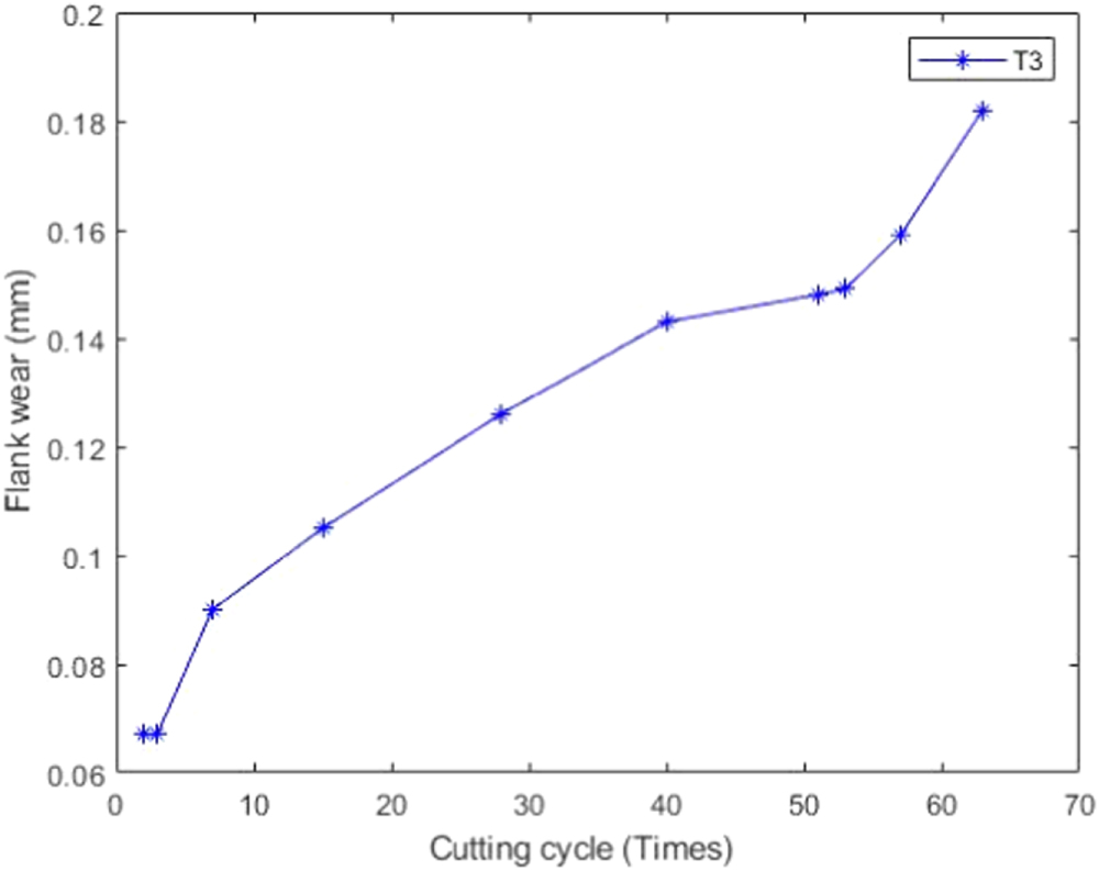
5. Conclusions and future work
The tool wear monitoring system was designed based on multi-sensor integration and depth residual network. Multi sensor signals were fused in the data layer through angle imaging technology, so that multi-channel time series data would be imaged into two-dimensional images. This method helped maintain the time relationship in the original signal on the premise of effective multi-sensor data fusion. In data processing, the residual convolution network with attention mechanism was used for feature extraction. The application of the residual convolution network proved to be able to improve the ability of the neural network to extract deep features, as well as to improve the robustness and performance of the entire feature extraction module. In the experiment conducted to verify the system, the results showed that the recognition accuracy is up to 90%, especially for rapid wear and severe wear.
In the future, we will seek for more reasonable combinations of sensor signals and dada fusion methods to improve the perception ability of tool wear condition. In addition, we will actively explore the applicability of other deep learning models in order to make the system more practical.
Acknowledgments
This research was financially supported by the National Natural Science Foundation of China (NSFC, Grant NO. 52275494) and the Natural Science Foundation of Shandong Province, China (Grant No. ZR ZR2021ME078).
Data availability statement
The data cannot be made publicly available upon publication because no suitable repository exists for hosting data in this field of study. The data that support the findings of this study are available upon reasonable request from the authors.