
Abstract
This is a Reply to the Comment of Dozias S., Pouvesle J.-M. and Robert E. on the paper 'Mapping the electric field vector of guided ionization waves at atmospheric pressure'. The criticism in the Comment, namely that the measurements and the subsequent interpretations are wrong, seems to be invalid. Additional information will be detailed to discuss the point of view of the authors. However, the criticism raises an interesting comparison of two data sets presented in a normalized color scale. The resulting figure clearly supports the argument that the plasma-induced electric field measurements are consistent and validates the experimental investigation.
Export citation and abstract BibTeX RIS
The Comment by Dozias S., Pouvesle J.-M. and Robert E. [1] raises concerns about the consistency of the experimental investigation of electric field (EF) distribution induced by guided ionization waves in Helium at atmospheric pressure [2]. With all due respect to the opinion of the authors, the claims in the Comment –namely that the results are wrong and inconsistent –seem to be invalid. However, the authors have suggested an interesting interpretation of the results which was missing in the original paper. A discussion in this direction will be detailed in this Reply.
Firstly, the authors seem to be confused with the meaning of secondary ionization wave (SIW) as they correlate it to their own works. In [2], the SIW is produced not because of the impingement of the IW onto a grounded target, but because of a rapid change of the applied potential at the electrode as shown in [3–5] on the total current evolution curve. Thus, this is not to be compared with so-called 'rebound'. Additionally, the external EF is a very sensitive quantity which does not require a direct interaction with a grounded target to be significantly affected. For instance, the data found in appendix of the PhD dissertation of Darny, T. (pages 256-258) and presented in the top left corner graph on page 257 exhibits a shape which recalls more the figure 2 of the original article [2] than the curve to be claimed in the Comment. The electric field is acting ahead of the IW propagation; this means that there is no need to have the IW directly in contact with the grounded plate to already induce a modification of the electric field and there is more research needed on this issue. Unfortunately, these data concerns the appendix and not the main core of the dissertation. The text is rather restricted to the description of the experimental conditions which limits a more thorough analysis.
Secondly, it is important to distinguish two aspects of the claim reported in the Comment:
- the angular position of the electro-optic (EO) probe to measure the EF,
- the consistency of the results presented after the analysis of the recorded signals.
Vector field and magnitude of the EF
The EO probe used in [2] is a customized commercial system produced by Kapteos
s.a.s. allowing for measuring simultaneously two orthogonal components of the EF at the exact same time and position in space [6]. This system involves a single crystal as part of the probe head. Recent development of this technology have led Kapteos
s.a.s. to re-engineer their system which means that the apparatus used in this study has been discontinued. The recorded data are Er
and Ex
, two vector components of EF from which one defines the magnitude of EF as,  . The sampling grid is defined as a Cartesian plane with
  -axis the vertical direction –parallel to the APPJ tube–and
  -axis the horizontal direction and aligned with the radius of the APPJ tube. Suggesting that the Ex
-axis is not parallel to the longitudinal axis of the APPJ would mean that an angle θ ≠ 0 (π) exists between the Ex
-axis of the probe and the
-axis the horizontal direction and aligned with the radius of the APPJ tube. Suggesting that the Ex
-axis is not parallel to the longitudinal axis of the APPJ would mean that an angle θ ≠ 0 (π) exists between the Ex
-axis of the probe and the  -axis of the sampled grid. Thus, the EF value on the longitudinal axis (
 ) and on the radial axis (
 ) of the APPJ are found according to the EO probe coordinate system (Er
,Ex
) as,
) of the APPJ are found according to the EO probe coordinate system (Er
,Ex
) as,


However, the magnitude of the EF,  is independent on a –hypothetical–angle θ (i.e by definition the magnitude of a vector does not depend on its direction [7]). Consequently and despite the protest of the Comment's authors, the filled contour plots displaying the EF magnitude in the original article [2] are algebraically exact. Note that this is correct for measurements performed with this specific two orthogonal axis EO probe. Nonetheless, this interpretation is not correct for measurements carried out with a more common single component EO probe. This was not mentioned in the original article [2] and may confuse the authors of the Comment. This Reply is a good opportunity to clarify the author's criticism and to prevent future readers of any possible misunderstanding.
Vector field and angular position of the EO probe
The verification of the angular position of the EO probe was argued in the original article [2], following the recommendation of one of the referee in charge. To argue against the measurements performed in [2] the authors compared the results presented in figure 1 and figure 2 in their Comment. The description of the experimental conditions is briefly mentioned; the authors present figures 1 and 2 showing measurement results acquired in the exact same conditions, except for the angular orientation of the probe. These are direct facts reported in the Comment. It is worth to mention the significant oscillations on both Ex (t) and Er (t) curves from 0μs to 1.5 μs only for the 45° tilt probe (figure 2 in the Comment) but not for the 0° tilt probe measurement (figure 1). It could be that some electric noise was also detected by the EO probe. One can hardly believe that it could result from a probe rotation only. Furthermore, both voltage curves have a time-shift of about 300 ns while the maximum of Ex (t)-curves is at 2.25 ± 0.05 μs in both diagrams. The 300 ns delay would correspond with an IW propagation pathway of 18 mm. These details raise some questions regarding the measurement conditions claimed to be identical in the Comment and show that there is still a need for future research on this topic.
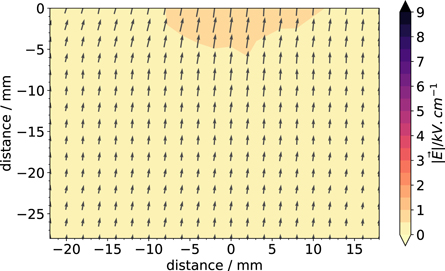
Figure 1. EF vector mapping presented in figure 4(a) [2] [t = 1.74 μs]. The quiver plot displays the vector EF arrows with components (Er , Ex ) centered at the points of the sampling grid. The filled contour plot shows the EF vector magnitude with a normalized color scale ranging from 0 kV/cm to 9 kV/cm. The axes' origin is reset at the tube outlet and centered on its vertical axis.
Download figure:
Standard image High-resolution image
Figure 2. Electrostatic simulation showing the EF streamlines of a spherical rode tip to plane geometry analogue to the situation shown in figure 4(a) [2] [t =1.74 μs]. (a) shows the EF streamlines in the asymmetric domain revealing the non-uniformity of the EF distribution on a large scale. (b) presents the EF streamlines in the experimental sampled domain shown in figure 1. The axis origin is reset at the tube outlet and centered on its vertical axis.
Download figure:
Standard image High-resolution imageAs explained in the initial article [2], the alignment of the EO probe axes with the longitudinal and radial axis of the APPJ is demonstrated in figure 1. At this precise time, the IW is far enough from the EO probe –in the vicinity of the electrodes according to figure 3(a) from [2], i.e. 50 mm from the ground metal plate—so that one can assume the hypothesis of the far-field approximation.
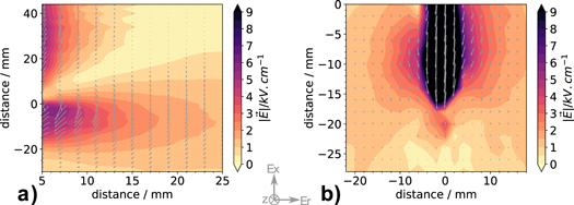
Figure 3. EF vector mapping initially introduced in [2] and currently displayed with a normalized color scale ranging from 0kV/cm to 9 kV/cm. (a) corresponds to figure 3(e) [t = 3.0 μs] and (b) to figure 4(g) [t = 2.9 μs] in the original article [2]. The axes origin is reset at the tube outlet and centered on its vertical axis.
Download figure:
Standard image High-resolution imageTo validate this hypothesis, an electrostatic simulation of the EF distribution is realized considering the following: in figure 4(a) [2] [t = 1.74 μs], the IW front is inside the tube, at least 22 mm from the exit (i.e. 50 mm from the ground metal plate). It can be approximated with a metallic rode tip of 2.0 mm radius of curvature (i.e. tube radius) and set to a negative potential. A grounded plate is placed 50 mm ahead of the spherical tip surface. By solving the Poisson's equation in the vertically asymmetric geometry, one computes the EF streamlines shown in figure 2(a). Similar computations have been reported in [8, 9]. More specifically the extended and comprehensive model of APPJ described in [10] shows simulations results of the EF vector distribution ahead of a negative IW in figure 7. The scale already gives an idea of the far-field assumption ahead of the IW.

Figure 4. Common sampled area of figures 3(a) and (b) plotted in an orthogonal basis as suggested by the authors of the Comment. The data are displayed with the same normalized color scale ranging from 0 kV/cm to 9 kV/cm. For clarity, sub-figures (a) and (b) are the regions of interest of figures 3(a) and (b) respectively. The axes' origin is reset at the tube outlet and centered on its vertical axis.
Download figure:
Standard image High-resolution image
It is usually accepted that probe diagnostics are more suitable for far-field investigations in low temperature plasma studies. This assumption is particularly valid as close as the probe approaches the grounded plate located at the position −30 mm. The far-field approximation is limited near the tube outlet, since a smooth magnitude gradient is hardly detected. This is explicitly shown in figure 1 displayed with a reduced color scale to reveal the homogeneous magnitude of EF over a major part of the sampling domain. Regarding the direction of the EF vectors, the quiver plot –showing the vector EF–draws arrows within the space coordinates of the sampling grid. Thus figure 1 is to be compared with figure 2(b) where the latter presents the computation results of the EF streamlines for the exact same space domain. Comparing both figures indubitably confirms the hypothesis of the far-field approximation particularly from positions −15 mm to −28 mm along the vertical axis. In the simulation as well as in the experimental data, the EF streamlines are quasi-uniform and supports the correct orientation of the EO probe. The small deviation angle which does not exceed 2° is within the experimental uncertainties of the measurements. This experimental evidence together with the electrostatic simulation support the validation of a trustful angular orientation of the EO probe criticized in the Comment. Note that the arrow's length representing each vector EF is set using a simple auto-scaling algorithm based on the average vector length and the number of vectors in one frame [11]. This means there is a significance to compare arrows relatively from the same frame as it is related to the magnitude. The latter also suggests that future applications of such probe may be done with additional calibration measurements in a defined electric field with a known field structure.
Comparison between experimental data sets and results consistency
The authors of the Comment proposed to compare the common area sampled in both domains and presented in figures 3 and 4 in the initial article [2]. This wise idea was missing in [2], but is indeed an interesting approach to explore. In their Comment, the authors present in figure 3 a direct comparison of the common areas. Unfortunately, the color scale of both initial figures mismatches which leads to hazardous interpretations. To support the initiative of the authors and to fully considered their comparison criteria, i.e. 'it is better to just compare the position of the maximum field, the gradients and the directions of the EF vectors.' [1], one chooses as a most representative example the pair of opposed sub-figures where the color gradient is high on one colormap and is –nearly–invisible on the other compared colormap. In this respect, a fair choice is figure 3(e) in the Comment [1]. Thus, one presents in figure 3 an example of EF vector mapping from the initial article [2] with the same color scale used in both cases. For better readability, the axes origin is reset at the tube outlet and centered on its vertical axis. While data shown in figure 3(a) matches the complete color scale range, figure 3(b) exhibits a saturated region along the path of the IW. In this condition, the common sampled area is selected and displayed in figure 4 with an aspect ratio of 1:1 for a rigorous comparison. The latter factually supports the argumentation that the EF magnitude distribution obtained experimentally in two different acquisitions are remarkably analogous. Apart from the minor time shift between the two acquisitions (due to the discharge jitter inherent to streamer nature), the EF gradient is remarkably the same within the measurement uncertainties. This comparison does support the consistency of the experimental data presented in [2], and highlight the coherence of the analysis of both sampled domains. Last, but not least, the authors of the Comment are gratefully acknowledged for this wise idea to compare the results and for the fruitful discussion developed in this Reply. The latter will bring additional missing information to the initial publication [2] which might mislead the early readers.
Acknowledgments
The author would like to thank the anonymous referee who provided detailed comments and fruitful discussions on the earlier version of the manuscript.
Data availability statement
The data that support the findings of this study are available upon reasonable request from the authors.