

Abstract
Super-resolution microscopy techniques have pushed-down the limits of resolution in optical imaging by more than an order of magnitude. However, these methods often require long acquisition times in addition to complex setups and sample preparation protocols. Super-resolution optical fluctuation imaging (SOFI) emerged over ten years ago as an approach that exploits temporal and spatial correlations within the acquired images to obtain increased resolution with less strict requirements. This review follows the progress of SOFI from its first demonstration to the development of a branch of methods that treat fluctuations as a source of contrast, rather than noise. Among others, we highlight the implementation of SOFI with standard fluorescent proteins as well as microscope modifications that facilitate 3D imaging and the application of modern cameras. Going beyond the classical framework of SOFI, we explore different innovative concepts from deep neural networks all the way to a quantum analogue of SOFI, antibunching microscopy. While SOFI has not reached the same level of ubiquity as other super-resolution methods, our overview finds significant progress and substantial potential for the concept of leveraging fluorescence fluctuations to obtain super-resolved images.
Export citation and abstract BibTeX RIS

Original content from this work may be used under the terms of the Creative Commons Attribution 4.0 license. Any further distribution of this work must maintain attribution to the author(s) and the title of the work, journal citation and DOI.
1. Introduction
The spatial resolution of optical microscopy is limited by the wave nature of light to around half its wavelength, that is 200 nm, for visible light. This limit was discovered by Abbe in 1873 [1] and for a long time was thought of as being insurmountable. In 1994, Hell and Wichmann realized that Abbe's limit can be circumvented by manipulating fluorophores such that the fluorescing volume is confined to below the diffraction limit [2], firing the starting shot in the race for far-field super-resolution microscopy.
Abbe derived the diffraction limit by describing the imaging system using classical linear optics and assuming the sample to be uniformly illuminated and stationary. Each of Abbe's assumptions corresponds to a loophole that can be used to overcome the limit [3]. Stimulated emission depletion (STED) microscopy [4] breaks the assumptions of linear-response and illumination uniformity, as does non-linear structured illumination microscopy (NSIM) [5]. Single-molecule localization microscopy (SMLM) methods such as photoactivated localization microscopy (PALM) [6] and stochastic optical reconstruction microscopy (STORM) [7] rely on the non-stationarity of the sample's fluorescence. Methods from the SMLM and STED families offer extreme resolution improvements down to a few nanometres [8].
It is evident that, owing to the breakthroughs in super-resolution microscopy and the impressive technological progress that followed, diffraction is no longer the limiting factor in fluorescence microscopy. Rather, it is the accessibility of super-resolution techniques in a given laboratory and their application to a specific biological problem that remains challenging. The high intensity required in STED can cause phototoxicity and fluorophore bleaching, which is problematic in live-cell imaging. Moreover, a complex laser setup drives the price of the system up. In the case of SMLM, long measurements limit the applicability to imaging dynamics in general and live-cell imaging in particular. Either microscopy family places high demands on the controllability and photo-stability of fluorophores. Last but not least, 3D super-resolution imaging, while possible, substantially increases the complexity of the experiment [9–12]. Due, in part, to these issues, most researchers continue to use standard, diffraction-limited microscopy methods.
Within the super-resolution toolbox, SMLM is arguably the most widely used class of methods. Since its main challenge is precise control of labeling density and fluctuation statistics, SMLM nicely fits into the standard workflow of biological light microscopy [13–15]. However, even with advanced labeling capabilities, live-cell SMLM microscopy is still very challenging [16] due to light-induced toxicity [17] and the relatively fast dynamics of the sample which blurs the super-resolved reconstruction. Since fluctuations are engineered to generate very sparse frames, thousands of frames must be collected to form a single super-resolved image. While devising denser scenes can speed up the image acquisition process, localizing overlapping emitters leads to substantial image artifacts [18, 19].
Nevertheless, due to dire need for faster super-resolution methods, in recent years we observed a constant progress towards denser frames and more sophisticated reconstruction algorithms [20, 21]. An alternative approach that tackles the challenge of dense frames is super-resolution optical fluctuation imaging (SOFI), introduced in 2009 by Dertinger, Enderlein and Weiss [22]. Similarly to SMLM, it relies on the fluctuations of fluorescing labels, but its contrast are the temporal and spatial correlations within the collected data. While the resolution enhancement it offers is typically smaller than that of SMLM and STED, it requires no special instrumentation and is less sensitive to the emitter density in the raw image frames, making SOFI a highly accessible super-resolution technique.
This review explores the evolution of SOFI from its original demonstration into a family of super-resolution methods that utilize correlations of fluctuations as their contrast. In section 2 we briefly describe the basics of SOFI and its classical implementation, starting with second-order auto-cumulants, through higher-order auto-cumulants, cross-cumulants, and closing with Wiener-deconvolution. Section 3 covers different aspects of the experimental setups that can be employed for SOFI imaging. We first focus on modalities that enable three-dimensional imaging and then move on to discuss the impact of detectors, including the potential of novel single-photon-avalanche detector (SPAD) arrays. Section 4 surveys different types of fluorescent labels compatible with SOFI. Finally, section 5 describes the standard data acquisition and analysis of SOFI and freely available data analysis and simulation packages. Moreover, artifacts typical for SOFI and ways to combat them are described.
Fluctuation-based imaging methods are applicable over a wider range of labeling densities than SMLM and can, therefore, contain a lot of information per frame. New ways of extracting this information are still being developed [19, 23, 24]. Recent algorithmic approaches to SOFI-like data are reviewed in section 6, starting from SMLM algorithms tackling overlapping emitters, through reconstruction of high-density frames to applications of deep learning.
Section 7 introduces the quantum analog of SOFI based on photon correlations in common labels. These rely on an alternative and complementary source of contrast, photon antibunching, which is purely a quantum effect, measured from the fluorescence of a labeled, complex, biological sample [25].
Finally, although SOFI is not yet a mainstream super-resolution technique, its relative simplicity enabled its applications to multiple biological studies. Selected examples are presented in section 8. Notably, SOFI has also been used to develop a new type of biosensor that uses fluctuations, rather than, for example, change in spectrum or fluorescence lifetime, as a measure of proximity [26].
While we limit the scope of the current review to microscopy methods that apply fluorescence fluctuations, it is interesting to note that the principles of SOFI have inspired multiple original imaging techniques that use fluctuations in the illumination pattern for super-resolution in fluorescence [27–30] and photo-acoustic [31–33] imaging. This choice of scope is not only a semantic distinction, rather it has an important implication on the resolution. In contrast to the independent fluctuations of neighboring emitters, illumination patterns are spatially correlated to the extent of the diffraction limit (of the illumination), the average size of the laser speckle. As a result, the resolution improvement limit of these techniques is two-fold, the same as that for linear structured illumination microscopy (SIM) [34] and image scanning microscopy (ISM) [35].
2. The original SOFI method
2.1. Overcoming the diffraction limit in fluorescence microscopy
Fluorescence microscopy relies on detecting light emitted from the sample after photo-excitation of fluorophores to a higher energy state with a light source such as a lamp or a laser. Absorption of light is followed by vibrational or conformational relaxation and emission of light at a longer wavelength. In a standard epifluorescence microscope (figure 1(a)), the same objective transmits the illuminating beam to the object and collects the emitted fluorescence. A dichroic mirror and dielectric filter separate the faint fluorescence from scattering and reflection of the illumination light and an additional lens (often referred to as a tube lens) images it onto a camera.
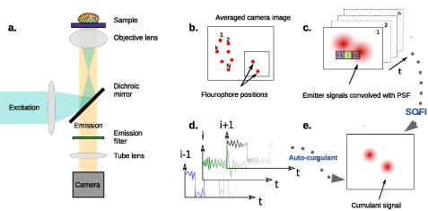
Figure 1. (a) Schematic representation of a wide-field fluorescence microscope. Excitation light is focused on the back focal plane of the objective lens to form a parallel illumination beam covering the entire field of view. Collected emission is separated from excitation with a dichroic mirror and imaged on a camera. (b)–(e) The principle of SOFI. (b) Emitter distribution in the object plane. Each emitter's temporal fluorescence fluctuation is independent of that of the others. (c) A series of images recorded by a camera. Each image is the convolution of the system's PSF with the emitted signal. Single emitters cannot be resolved when two or more PSFs overlap such that the distance between their centers is less than the diffraction limit. (d) Each pixel contains an intensity time trace consisting of the sum of individual emitter signals whose PSFs reach that pixel. The second order auto-correlation function is then calculated from the fluctuations at each pixel. (e) The SOFI intensity value, assigned for each pixel, is given by the integral over the second-order correlation function. The SOFI image resolution is higher by a factor of  .
.
Download figure:
Standard image High-resolution imageThe resolution of an image captured with an optical microscope is limited by diffraction. This stems from the wave-like character of light: no matter what kind of optical components we use, we cannot focus the light waves beyond about half of its wavelength. As, a result, the image of a point object is not a single point but a finite-sized blur that we term the point spread function (PSF). The shape of the PSF depends on the properties of the imaging system and can be calculated knowing its geometry. In particular, the PSF of a circular lens is an Airy disc—a circular pattern with a bright center spot and alternating bright and dark rings [36]. The first dark ring appears at a radius of  , where λ is the wavelength of light and
  is the numerical aperture of the lens, described in the following paragraph. The Rayleigh criterion attempts to provide a simple quantitative metric to the complex concept of resolution. According to it, two imaged objects can be distinguished from each other if the distance between them is longer than the radius of the first dark ring in the Airy disc. Otherwise, the Airy discs merge together and cannot be resolved.
We now present a complementary discussion, generalizing the topic of resolution and its enhancement in terms of spatial frequency content, i.e. the Fourier transform of the object or image. Because of its finite size, an objective lens collects light rays emerging from the sample up to some maximal angle, θ0, from which we derive the numerical aperture,  (n is the refractive index of the medium). In a simplified yet constructive picture, this angle directly translates to the maximal spatial frequency that propagates from the object to the image,
  . Higher spatial frequency content is lost in this propagation and as a result the finer details of the object do not translate to the image. In image processing, one would refer to this process as a short-pass filter with a cut-off frequency of
  . Putting it all together, to simulate the imaging system, the object should be Fourier transformed, its content set to zero at frequencies beyond
  and finally inverse Fourier-transformed back into real space. A thorough, yet intuitive, explanation for this mechanism is given in the review in reference [37].
A fluorescence image is proportional to the light intensity (incoherent), a time-average of the electric field squared. In the Fourier domain, this squaring translates to a convolution of the frequency filtered PSF with itself, containing spatial frequencies up to  . More accurately, to calculate the fluorescence intensity image, we multiply the frequency content of the sample with the modulation transfer function (MTF) which becomes zero for
  , the cut-off frequency. Unlike the simplified coherent case, the MTF strongly depends on k even within the
  region, suppressing the contribution of higher spatial frequencies (see figure 3(a)). This dependence of the MTF on k will be discussed in greater detail in section 2.4. Circling back to the image position space, the PSF is simply the Fourier transform of the MTF. Thus, extending the frequency cut-off translates to a narrower PSF and higher resolution.
Super-resolution microscopy can be framed as an attempt to narrow the image PSF (or extend the MTF cut off) beyond the Abbe diffraction limit and therefore resolve features that are closer together than  . The 2014 Nobel prize in Chemistry was awarded for the development of two groundbreaking super-resolution methods that revolutionized far-field light microscopy. The earliest, STED, uses the non-linear response of labeling emitters to light by saturating their excitation depletion with a doughnut-shaped beam. As a result, only emitters at the very confined space at the center of the scanned doughnut contribute to the signal and the effective PSF is significantly shrunk.
Perhaps the most wide-spread approach for super-resolution, SMLM, relies on fluorescence fluctuation of emitters. These randomly shine for a short enough period of time so that they mostly do not overlap with each other in any frame. Collecting the precise position of these emitters over a long video produces a substantially sharper image than the averaged image. The following sub-section describes the PSF narrowing mechanism of another successful super-resolution method that relies on fluorescence fluctuations, SOFI—the subject of this review.
2.2. Cumulants of intensity fluctuations for super-resolution
2.2.1. Second-order SOFI
In practice, the intensity of light emitted from a fluorophore is typically not constant in time. Repeated transitions between a fluorescent and non-fluorescent state lead to intermittent emission or blinking that can be exploited for obtaining sub-diffraction images. SOFI relies on recording a movie of a sample and analysing the changes of its fluorescence intensity in time. This image series is then processed into a single correlation image with increased resolution.
Consider a two-dimensional sample consisting of N independent emitters whose time-dependent brightness is given by  , where rk
is the emitter's location,
, where rk
is the emitter's location,  is the constant molecular brightness and
  is the time-dependent component with values between 0 and 1 (figure 1(b)).
The time-dependent fluorescence image at position r is a convolution of the microscope's PSF  with the sample brightness,
  (figure 1(c)):

We explicitly assume here that the positions of emitters do not change during the measurement and temporal changes are caused only by blinking.
Wide-field microscopy employs time average over  , which is a sum of averaged contributions from each emitter multiplied by
  . Contrariwise, a SOFI image is derived from correlations of the time dependent signal (figure 1(d)). In the most basic form of SOFI, it can be shown [22] that the second order auto-correlation function
  already provides a
  improvement in resolution (figure 1(e)). To mathematically observe that we can write the full expression for the auto-correlation of the fluorescence intensity:

where  denotes time averaging and
  describes the fluctuation, i.e. the difference with respect to the average intensity at a given time. Note that, we assume here that emitters fluctuate independently of one another, i.e. the emission of any two emitters is uncorrelated in time. As a result, cross terms proportional to the product of two different emitters' intensities
  , for i ≠ j, average to zero and equation (2) contains only a single sum over emitters.
The key difference between the correlation contrast in equation (2) and the wide-field contrast in equation (1) is the presence of a squared PSF. Raising the PSF to a higher power results in the appearance of sharper features in the image, hence super-resolution (see figure 2(a)). In particular, for a Gaussian-shaped PSF (often a good approximation), squaring the PSF corresponds to a reduction of width by a factor of  . Moreover, this reduction happens in all three dimensions, thus increasing the resolution of the SOFI image in 3D. A comprehensive discussion on 3D resolution is included in section 3.1. An additional advantage of SOFI, reflected in equation (2), is the fact that any non-fluctuating background signal vanishes on average.

Figure 2. A demonstration of super-resolution in SOFI. Panels (a), (b), and (c) have been adapted from figures 2, 3, and 4 of [22], respectively. (a) Higher-order SOFI images. Selected SOFI images acquired for a sparse sample of quantum dots (QDs) are shown. From upper left to lower right: original image (mean intensity of all movie frames) and 2nd, 4th, 9th, 16th, and 25th orders of SOFI. The two different QDs are resolved at higher-order SOFI images. The dotted cross-section lines are used in (b). (Scale bars: 250 nm.) (b) Resolution enhancement of SOFI. Fitted FWMH (circles) as a function of cumulant order, as obtained from the Gaussian fits of the cross sections displayed in (a). The fit shows a  resolution improvement for the nth order cumulant. (b) 3D SOFI 3D PSF obtained from a 3D scan through a single QD (300 nm spacing along the z axis). The smoothed e−2 isosurfaces are shown. Starting from the outermost isosurface, the original PSF is shown followed by orders 2nd, 3rd, 4th, and 16th. This demonstrates that the SOFI's PSFs are shrinking along all three axes at higher orders. Reproduced with permission from [22].
Download figure:
Standard image High-resolution imageThe reader may recall (section 2.1) that squaring the PSF can be interpreted as a convolution of the MTF, the Fourier transform of the PSF, with itself. Indeed, the auto-correlation image (equation (2)) includes a squaring of a PSF in real space and therefore corresponds to convolution in the Fourier domain and an extension of the spatial frequencies cut-off up to  (see the MTF simulation in figures 3(a) and (b)). The presence of higher spatial frequencies results in narrower features in the image and is therefore a complimentary indication of super-resolution (see figures 3(f) and (g)). While these features hint that a super-resolved image can, in principle, be reconstructed, some caution is required since the mere presence of higher frequencies does not always mean that the image is true to the original sample structure and artifacts may create distortions. The spatial frequency point-of-view on resolution will become critically important when discussing higher correlation orders in the following section and deconvolution in section 2.4.
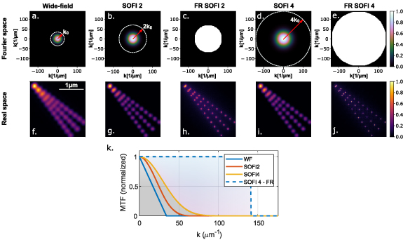
Figure 3. PSF, MTF and Fourier re-weighting (FR) in SOFI. ((a)–(e)) Simulated 2D modulation transfer functions (MTF) for wide-field (a), 2nd order SOFI (b), FR 2nd order SOFI (c), 4th order SOFI (d) and FR 4th order SOFI (e). A 500 nm wavelength and an objective lens with an  of 1.4 were used in the simulation. The white dashed circles denote the frequency cut-off for each method. Despite the dashed line radii linear increase with SOFI order, we note that without FR the gap between reasonable amplitude (e.g. 0.1) and the frequency cut-off increases from wide-field to 2nd order SOFI to 4th order SOFI. The strength of FR, as evident in (c) and (e) where the amplitude of the high frequency content is digitally amplified. ((f)–(j)) A simulated image corresponding to the MTF in ((a)–(e)), respectively. While FR narrows the main lobe of the PSF, an unavoidable halo develops due to secondary rings in the PSF. (k) A cross-section of the MTF for wide-field, 2nd order SOFI, 4th order SOFI and FR 4th order SOFI at
  .
.
Download figure:
Standard image High-resolution image2.2.2. Higher-order SOFI
The above description can be generalized to higher correlation orders. These contain frequency components beyond the cut off of the second-order correlations and therefore have the potential to increase the resolution even further. However, the presence of the cross-terms (multiplications of PSFs from different emitters) may yield sharp features that do not reflect the shape of the underlying object. To remedy this, SOFI analysis uses cumulants, rather than correlations, eliminating the contribution of cross-terms. The nth order cumulant, a linear combination of correlations up to the nth order, is described by a recursive formula given in reference [38]. Once cross terms have been eliminated, the resulting nth order SOFI image is given by:

where  is the single-emitter cumulant of the nth order.
Analogous to the second-order expression, equation (3) contains the PSF raised to the power of n. This implies that for a Gaussian PSF, the resolution improvement is by a factor of  (see figures 2(a) and (b)). Although, in theory, there is no limit on the calculated cumulant order and the corresponding resolution improvement, there are in fact, some practical aspects that limit the application of higher-order SOFI. In general, higher orders require longer measurements and are more sensitive to noise. This, in turn, entails increasing the exposure time, illumination intensity or number of acquired frames. All these changes have significant drawbacks including higher fluorescence bleaching, susceptibility to sample drift. Moreover, small variations in molecular brightness,
  , also raised to the nth power, are translated to an increasing signal range with higher orders resulting in the image being dominated by the brightest emitters. Finally, there are some considerations specific to SOFI such as artifacts resulting from different blinking statistics of neighbouring fluorophores. These topics are discussed in detail in section 5. Recent theoretical analyses show that it is not trivial to quantify the amount of added information in fluorescence cumulants of different orders [39, 40].
2.3. Extension to cross-cumulants
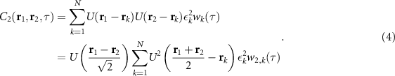
Until now we have discussed auto-cumulant-based resolution enhancement, obtained through computing temporal correlations at a single position. This description can be generalized to cross-cumulants obtained from spatio-temporal correlations. Let us first consider the second-order cross-cumulant between positions r1 and r2 for a Gaussian-shaped PSF [41]:
Two things stand out here. First, a cross-cumulant between  and r2 results in a signal in the geometric center of these two points
  . Second, the expression is multiplied, or weighted by a 'distance factor'
  . The latter can be understood intuitively: since emitters fluctuate independently, only points within the same emission PSF can contain contributions from the same emitter and have a non-zero correlation.
The significance of a signal generated at the geometric center of the two positions becomes apparent when we consider a real-life camera with discrete, finite-sized pixels. If we acquire an image series and calculate auto-cumulants of increasing orders, eventually the pixel size will limit further resolution improvement. In contrast, by calculating cross-cumulant of neighboring pixels, we create additional 'virtual pixels' and increase the pixel density. Contrary to a simple interpolation, these pixels carry additional information. The process of creating virtual pixels is further discussed in section 5.1.
Similarly as for auto-cumulants, equation (4) can be extended to higher orders, up-sampling the image even further. The nth order cross-cumulant will theoretically yield an n × n-fold up-sampled SOFI image [41].
2.4. Enhancing super-resolution with Wiener deconvolution
Fourier reweighting (FR), sometimes also termed Wiener-deconvolution or Wiener-filtering, is a post-processing step that attempts to stretch the resolution of an image to its optimum. Its application to further enhance SOFI images was proposed very soon after SOFI's initial demonstration [41].
In order to describe FR and its benefits, it is helpful to look at the topic of image resolution from the spatial-frequency domain point-of-view, introduced in section 2.1. The PSF of an nth order SOFI image contains spatial frequencies up to  , where k0 is the spatial frequency cut-off of the diffraction-limited image, with higher frequencies corresponding to sharper features in the image. In contrast, the resolution of SOFI increases at a much less favorable scaling of
  . To understand this discrepancy, we look beyond the frequency cut-off and observe the functional form of the MTF, the Fourier transform of the fluorescence (incoherent) PSF (see section 2.1). To illustrate this delicate point, simulated MTFs (500 nm wavelength, 1.4
  ) are presented in figures 3(a)–(e) (cross-sections in figure 3(k)) for diffraction limited imaging and different orders of SOFI and their FR version. The cut-off frequency, beyond which the MTF becomes identically zero, for each method is denoted as a white dashed circle whose radius grows linearly with the order. However, the gradient with which MTF approaches zero is quite different for the different methods: the decrease of amplitude with spatial frequency is more rapid for 2nd order SOFI than it is for the diffraction limited version and is even more rapid for the 4th order SOFI. For example, comparing the simulated MTF of a diffraction limited image (3(a)) and that of 2nd order SOFI MTF (3(b)), one can observe that while the cut-off frequency (white dashed circle) increases by a factor of 2, the reasonable amplitude portion (e.g. normalized amplitude greater than 0.1) did not expand as much and appears further away from the cut-off. This gap between the frequency cut-off and frequencies with reasonable amplitude MTF grows even further when observing 4th order SOFI (3(d)). As a result, the resolution scales in a sub-optimal
  manner with the order in non-FR versions of SOFI [41] and ISM [35].
Theoretically, this can be amended by simply multiplying the Fourier transform of the image with the inverse of the MTF for the appropriate SOFI order,  , for any
  . In practice, however, one has to consider the changes to signal-to-noise ratio (SNR) in the final image. Roughly speaking, SNR is the ratio between the measured signal level (e.g. pixel value in a camera image) and the average deviation under multiple repetitions of the measurement. Typically, SNR increases with the level of signal. In the Fourier domain, the MTF sharply decreases with frequency, corresponding to a lower signal and a lower SNR at high frequencies. Digitally amplifying those higher frequencies enhances the resolution, but at the same time increases the content of noise in the image. A standard approach to manage the resolution-SNR trade-off is using a Wiener-filter in the Fourier domain:

where k is the spatial frequency, and the parameter ξ is typically manually adjusted, using higher values for low SNR images. Here, a direct relation is created between the SNR of the image and its resolution; for a low SNR image a high value of ξ is required and the amplification of higher frequencies is moderate. Thus, nth order SOFI image may not achieve the potential × n resolution increase. A simulated demonstration of the resolution improvement through FR (inspired by [41]), for diffraction limited image, 2nd and 4th order SOFI and their FR versions, is given in figures 3(f)–(i).
Some practical consideration should be taken when applying FR. Estimating the PSF of an imaging system, experimentally or theoretically, is not a trivial task and errors in estimation would lead to image distortions. In theory, given an independent source of added noise, ξ would be the frequency dependent inverse of the image SNR [42]. Nonetheless, in low signal fluorescence microscopy camera noise is often not additive (e.g. shot noise) and the SNR is difficult to estimate. Using a constant parameter or a linearly increasing function of k have been shown to achieve near optimal resolutions expected for high SNR images [25, 35, 43].
2.5. SOFI compared to other super-resolution techniques
In the previous sections we have described the principles and basic properties of SOFI. From a practical point of view, it is natural to ask how SOFI compares to other already established super-resolution imaging methods. A detailed comparison of different methods can be found in numerous reviews, including some recent ones that take into account latest developments in the field [37, 44, 45]. Here we will provide a short summary to give the reader an idea of where SOFI lies in the super-resolution microscopy landscape.
There are many criteria by which super-resolution imaging methods can be compared. The most obvious one is resolution, both lateral and axial. SOFI can offer lateral resolution improvement beyond the x2 that ISM and linear SIM can provide and an equivalent improvement to that of NSIM. However, although theoretically SOFI PSF narrowing can be arbitrarily large, if high-order cumulants are computed, the resolution achieved in practice is not as high as that of STED or SMLM, where molecules can be localized with lateral resolution close to their size, i.e. 10–20 nm. Axial resolution is a separate issue. Many of the early super-resolution microscopy approaches focused on thin samples and operated only in lateral direction, offering little or no improvement of the axial PSF. Moreover, in biological samples the imaging depth is restricted by the ability to reject out-of-focus light that otherwise produces a background detrimental to image quality. This is an issue especially for methods with camera-based detection, such as SOFI, but also most SMLM implementations. Optical setup modifications that address this are described in section 3.1.
While newer implementations of STED and SMLM offer superior resolution in 3D, this comes with trade-offs, discussed in detail by Schermelleh and co-workers [45]. STED requires high light intensity to maximally depopulate the excited state, which can lead to photodamage. A similar problem is met when performing NSIM which requires a high laser power in order to achieve saturation. Since STED is a scanning method, high resolution dictates a small scan step and a long acquisition time. Similarly, for SMLM reconstruction a high number of raw data frames is required for one super-resolved frame. As a result, out of methods that are readily applicable to dynamic processes as well as live sample imaging, fluctuation-based techniques are those that offer the highest spatial resolution. Indeed, most of the life sciences applications of SOFI that we list in section 8 use it for live imaging.
Finally, the complexity of a method is another important consideration. From the optical setup point of view, SOFI is very simple to realize: it is sufficient to record a series of frames instead of a single one. This makes it simpler than methods such as SIM and STED that require shaping of the excitation light. On the other hand, like SMLM, SOFI leverages the fluctuations of the sample itself. This means that a fluorophore with blinking behavior on a timescale comparable to the acquisition frame rate must be chosen and labelling density has to be adapted. While these requirements are a limitation, they are less strict for SOFI than those of SMLM, as SOFI can better deal with multiple emitters close together [46].
3. Modifications to the microscope setup
The initial demonstrations of SOFI were done with a conventional wide-field microscope and noted ease-of-use, background rejection and high SNR as part of their advantages over contemporary super-resolution techniques [22, 47]. The simplicity of the optical setup, loose requirements from the labels and robustness enable its combination with various microscopy techniques, including emerging methods such as on-chip microscopy [48] and techniques with demanding experimental conditions such as cryogenic electron microscopy [49]. Importantly, the simple integration with existing microscopy techniques can be targeted to overcome some of the limitations of the original demonstration. Namely, its applicability to bio-imaging is limited mainly due to insufficient Z-sectioning and low SNR for short exposures. This section explores modifications to the optical setup and camera technology that attempt to tackle these issues.
The following section 3.1 reviews total-internal reflection (TIRF) microscopy, light-sheet microscopy (LSM) and confocal microscopy in combination with SOFI as robust solutions to 3D super-resolution. Section 3.2 discusses the use of different types of imaging sensors for SOFI and their influence on the SNR (or exposure time): electron multiplying charged-coupled device (EMCCD), scientific complementary metal oxide semiconductor (sCMOS) cameras and the developments in SPAD arrays and the potential that they hold for fluctuation-based microscopy.
3.1. Achieving 3D imaging with SOFI
One of the main limitations of wide-field microscopy is a lack of Z-sectioning (sometimes termed optical sectioning)—the ability to reject out-of-focus light. Consider a three-dimensional, fairly uniform, sample of fluorescent labels under wide-field excitation (figure 4(a)). While only a specific plane is perfectly focused on the camera, each plane in the sample contributes the same amount of light to the image plane. Although the details of these out-of-focus planes are blurred, their high overall intensity overwhelms the faint contribution of the focused features. Thus, samples thicker than a few microns are very difficult to image in this manner.
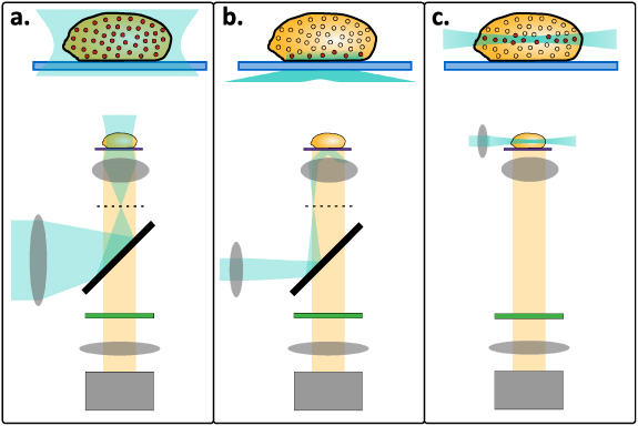
Figure 4. Imaging modalities for camera-based SOFI acquisition. Upper: a thick sample with excited emitters marked in red. Lower: a schematic of the microscope setup, including excitation (blue) and emission (yellow) beams as well as the optic used for excitation. (a) Wide-field microscopy. All the emitters in the sample are excited and imaged at the same time, no Z-sectioning. (b) Total internal reflection fluorescence (TIRF) microscopy. Evanescent wave is created and illuminates a thin section of the sample adjacent to the microscope slide. (c) Light-sheet fluorescence microscopy (LSFM). Excitation beam is formed into a thin 'light sheet' that illuminates a section of the sample from the side.
Download figure:
Standard image High-resolution imageA mathematical formulation of the problem is readily achieved by considering the 3D PSF as a Gaussian beam:

where r and z are the radial and axial coordinates, respectively. The z-dependent beam width,  , is defined by the w0 and zR
parameters, termed the beam waist and Rayleigh range, respectively. If we would image a 3D sample with uniform label density in all directions the contribution of each xy plane would simply reduce to an 2D integral over
, is defined by the w0 and zR
parameters, termed the beam waist and Rayleigh range, respectively. If we would image a 3D sample with uniform label density in all directions the contribution of each xy plane would simply reduce to an 2D integral over  . A reader who is familiar with Gaussian functions can already notice that regardless of the function w(z), integrating over the xy plane yields a constant independent of z. This means that in wide-field microscopy every z-section generates the same integrated intensity, whether it is in the focal plane or quite far from it. Therefore, when imaging a standard biological optically-thick sample with widefield illumination, the signal originating from the focal plane is just a small fraction of the entire observed fluorescence.
Two popular methods that overcome this critical issue are confocal and two-photon microscopy [50, 51]. While the physical mechanism behind these methods vary, from a purely mathematical standpoint, the effective PSF in both is a square of the wide-field PSF (at the wavelength of excitation) [51]; as if the pixels were sensitive only to two simultaneously arriving photons originating from the same emitter. As a result, the signal from out-of-focus emitters, whose emission is spread-out over a large area in the image plane, rapidly decreases with their distance from the focal plane.
Now, if we repeat the reasoning above for a case where the effective PSF is  (e.g. confocal microscopy and two-photon microscopy), the signal from a plane at a height z is:

Here, with growing distance from the focal plane, as the beam expands (w(z) increases), the integrated intensity contribution, I(z), reduces, thus sectioning the imaged sample around the focal plane.
A second-order SOFI image, computed through correlations, also yields an effective squared PSF and therefore provides Z-sectioning that is theoretically as good as in confocal and two-photon microscopy. This property of SOFI has been shown by three-dimensional imaging of a single quantum dot (QD) [22] as well as few-micrometers-thick cells [47] (see figure 2(c)). Yet, practically, Z-sectioning generated through post-processing cannot perform as well as optical sectioning. While the out-of-focus contribution averages to zero a finite-time measurement includes noise which directly translates to unwanted noise in the correlation signal.
Nevertheless, a good example of the inherent 3D potential of SOFI alone can be found in live-cell 3D imaging with a multi-plane wide-field fluorescence microscope [52]. Multi-plane imaging was realized by splitting the emitted light into eight parts and imaging different optical planes onto different regions of two sCMOS sensors. Next, 3D cross-cumulants were calculated for pairs of consecutive depth planes. This approach results in a more homogeneous contrast along the optical axis compared with sequential plane-by-plane 2D cross-cumulants. However, it requires a complicated setup that is sensitive to misalignment as well as carefully selected low-noise detectors.
Imaging of thick samples is a crucial problem for light microscopy in general and for most super-resolution microscopy methods in particular. In that respect, implementing SOFI in conjunction with an optical solution for Z-sectioning is a straightforward way to overcome this challenge.
3.1.1. Total internal reflection fluorescence (TIRF) microscopy
As far as live-cell imaging applications are concerned, the combination of SOFI with total internal reflection fluorescent microscopy (TIRF) has been demonstrated to work well. In TIRF, evanescent wave illumination with finite depth (figure 4(b)) provides optical sectioning and at the same time reduces phototoxicity [53]. Typically, total internal reflection occurs at the interface between glass and water-based medium surrounding the sample by a laser beam entering a high-numerical-aperture objective off-axis; a high NA is required to exceed the critical angle. Fluorescence excited by the evanescent wave is then collected with the same objective and recorded with a camera. In fact, most in vivo SOFI experiments mentioned in this review have been performed in a TIRF microscope.
3.1.2. Light-sheet fluorescence microscopy
While TIRF microscopy offers excellent Z-sectioning, its main limitation is the ability to image only a few-hundred-nanometre-thin layer at the interface where the evanescent wave is formed. This implies, for example, that only the membrane of a several-micrometre-large cell can be imaged and not the cell nucleus.
An alternative approach to optical sectioning suitable for thick samples is light-sheet fluorescence microscopy (LSFM). In this configuration, the excitation beam is focused into a two-dimensional 'sheet' and illuminates the sample along an axis perpendicular to the imaging objective axis (figure 4(c)). The signal from the illuminated plane is then detected by a camera. LSFM enables imaging at any depth in the sample, limited only by scattering. Despite other challenges, such as the need to redesign the microscope setup to accommodate two perpendicular optical axes as well sensitivity to refractive index mismatch, LSFM is steadily gaining popularity in a broad variety of applications [54].
The combination of LSFM and SOFI was demonstrated for the first time in a two-photon light sheet microscope, where the sheet is realized by scanning a beam focused to a line. In this work, the cells were stained with a QD-conjugated antibody and a reconstruction using 4th-order SOFI resulted in a 3-fold resolution improvement [55].
Recently, Mizrachi and co-workers have shown that a commonly used dye, Alexa Fluor 488, exhibits millisecond-scale blinking when used for CUBIC-cleared samples. The authors obtained super-resolved images of thick mouse brain sections by performing deconvolution with a 3D PSF and then computing cumulants up to the 10th order [56]. This is a unique demonstration of higher order SOFI in biological tissue that could open a potential road to a wider application of SOFI in cleared samples without the need of modifying the established staining protocols.
3.1.3. SOFI in scanning mode
Since super-resolution in SOFI relies on the temporal analyses of collected fluorescence, its principle can be applied together with multiple microscopy geometries. In this section, we discuss the combinations of SOFI with scanning microscopy techniques. The most straightforward example is combining the SOFI with confocal laser scanning microscopy (CLSM). In standard CLSM, the sample is illuminated with a focused laser beam and fluorescence collected through the same lens is focused onto a small pinhole (see figure 5(a)). Since only light from the point conjugate to the pinhole (at the focal plane of the objective) is efficiently transmitted through it, most of the signal from other planes is rejected [58, 59]. CLSM offers optical sectioning with a simple experimental setup.

Figure 5. SOFISM. (a) A schematic of a scanning microscope. (b) The mechanism of resolution enhancement in ISM. The probability of detection (green circles) for each detector in the array (black circles) is a multiplication of the excitation beam profile (blue circle) and the detection probability (red circles). Note that the resulting effective PSF for each detector is shrunk by a  and shifted. (c) The CLSM, ISM and SOFISM images of QD-stained microtubules. (b) Reprinted by permission from Springer Nature Customer Service Centre GmbH: Springer Nature, Nature Photonics. [25] (2019). (c) Reproduced from [57]. CC BY 4.0.
Download figure:
Standard image High-resolution imageA major disadvantage of CLSM is that acquiring a scanned image, especially in 3D, is time-consuming. To perform SOFI analysis of a CLSM image, one needs to sample the intensity signal at multiple time windows for each single scan step while keeping the entire scan process reasonably fast. For this, a high temporal-resolution detector such as a photomultiplier tube (PMT) or SPAD is required.
Conceptually, the combination of SOFI analysis with a CLSM system provides a robust super-resolution imaging method that maintains the capacity of CLSM to perform 3D imaging [57]. However, due to the point-by-point scanning mode, the acquisition time of such a combination is substantially longer than that of conventional SOFI. As a result, this combination has not yet been experimentally demonstrated.
Image scanning microscopy (ISM), a super-resolved variation to CLSM introduced in recent years, had become a widespread approach to achieve a moderate super-resolution within standard microscopy acquisition times [35, 60]. In ISM, the confocal pinhole is replaced with a detector array containing a few tens of pixels. As schematically shown in figure 5(b), the ISM PSF for each pixel (green) is a multiplication of the laser focus (blue) and the detection probability during the scan (red). This results in a  narrower PSF that can be translated to a
  resolution enhancement through deconvolution (see section 2.4).
Analyzing the classical [57] or quantum [25] fluctuation contrast in an ISM architecture results in an effective PSF for each detector pair that is even narrower than that of ISM, yielding a  improvement in resolution [25, 57] for 2nd order SOFI. A comparison of CLSM, ISM and SOFISM (super-resolution optical fluctuation ISM) images analyzed from the same measurement is shown in figure 5(c) [57]. In addition to increased lateral resolution, an improvement in Z-sectioning is achieved in SOFISM. Moreover, reasonable SNR images could be obtained within a short
  ms exposure time per pixel, far less than the 10's of seconds commonly required for 2nd order SOFI with a camera. This improvement is attributed to the ability of such SPAD detector arrays in sensing fast intensity fluctuations (see section 3.2.2 for an in-depth discussion).
In principle, just like ISM [43, 61], SOFISM can be performed in a multi-beam architecture (for instance in conjunction with a larger SPAD array [62]) and can even be complimented with a two-photon excitation scheme. We expect that such a combination would achieve  super-resolved images with more than 1 FPS deep within a tissue.
Finally, the combination of camera-based SIM with both quantum [63] and classical [64] fluctuations was suggested as an alternative pathway to wide-field super-resolution beyond the ×2 enhancement of structured illumination. Very recently, the combination of SIM and SOFI has been demonstrated experimentally, achieving up to 2.4-fold image resolution increase for imaging of fixed cells [65].
3.1.4. Spinning disk confocal microscopy
The elegant solution of confocal microscopy to the 3D microscopy challenge comes at the price of a serial image acquisition through the process of scanning. One approach developed to solve this trade-off is the spinning disk (SD) microscope [66]. In a modern SD microscope, a laser beam is focused through a rotating wheel of microlenses onto a second wheel of pin-holes. Fluorescent light passes back through the pin-hole wheel and is image onto a camera. This effectively generates a multi-beam implementation of a confocal microscope in which the beams are scanned through the synchronized rotation of the two wheels.
SOFI can be implemented within an SD microscope by simply calculating the cumulants of the resulting image stack. Such an implementation was indeed achieved employing an up to 4rd-order SOFI analysis for a fixed cell samples labeled with QDs, dyes and fluorescent proteins (FPs) [67, 68]. However, since an SD microscope still requires a full wheel rotation to achieve a single frame its frame rate is typically  10 Hz. As a result, only relatively slow fluctuation can be captured in such a setup, limiting its SNR and ease-of-use. The z-sectioning performance of an SD microscope is not as impressive as those of a CLSM microscope due to optical cross-talk between different holes in the array which introduce out-of-focus contributions.
3.2. The influence of an imaging sensor on SNR
One of the important elements of an imaging system is the camera sensor, making a significant contribution to both the quality and the price of the microscope. Since SOFI relies on image correlations, its requirements from an imaging sensor are somewhat different than those of other super-resolution microscopy methods. The application of currently available commercial microscope camera technologies, EMCCD, CMOS and sCMOS, is discussed in section 3.2.1. A possible future technology for SOFI microscopy, SPAD arrays, is described in section 3.2.2. Specifically, we consider the potential of high temporal resolution in SPADs to enhance the SNR of SOFI.
3.2.1. Established camera technologies—EMCCD, CMOS, and sCMOS
In this section, we discuss the technical differences between EMCCD, CMOS, and sCMOS cameras and their compliance with the SOFI method.
First, we briefly describe the main technological differences between the different types of cameras. The chip of an EMCCD is equipped with a single on-chip electron multiplying register prior to the signal readout, enabling detection of single photons without an image intensifier. In fact, the commercialization of EMCCDs was a catalyst for the development of super-resolution microscopy, enabling, for example, the localization of single emitters from a weak signal of hundreds and even tens of photons per frame [69]. In CMOS and sCMOS sensors, each pixel consists of a photodetector and a surrounding circuit. Since CMOS cameras are cost-effective and offer a low-power consumption, they are often found in consumer products such as smartphones and web cameras [70]. sCMOS cameras are the latest-generation CMOS image sensors developed particularly for low-light applications such as fluorescent microscopy. They are characterized by low noise, a large number of pixels, and a high quantum efficiency, and frame rate [71].
Following the work of Van den Eynde et al [72], we compare EMCCD, sCMOS, and CMOS cameras performances in SOFI and discuss their parameters. We note that as compared to sCMOS and EMCCDs, currently, CMOS cameras are cheaper by more than an order of magnitude.
Since SOFI relies on an analysis of emitter fluctuations, one of the most important camera parameters for its performance is the frame rate. sCMOS cameras present a higher frame rate than EMCCD sensors that typically reach 50–90 fps with 512x512 pixels ROI (e.g. iXon Ultra 888, Andor or ImagEM X2, Hamamatsu), while high-end sCMOS like Flash (Hamamatsu) or Zyla (Andor) can achieve 400 fps for similarly sized ROIs (100 fps with full 2048x2048 pixels frame). Considering the similar technology, it is not surprising that standard CMOS cameras (for example, BlackFly series from FLIR) support rates of hundreds of frames per second for ∼0.5 mega pixels. As described in section 4, most types of emitters contain fluctuations at shorter time scales than those typically measured in standard SOFI and SMLM experiments. As a result, high frame rate can be very beneficial for SOFI analysis and CMOS-based cameras offer a clear advantage in this category. We note, that this rather intuitive claim was, to our knowledge, not meticulously studied up to date.
Another frequently discussed camera parameter is quantum efficiency (QE). EMCCD sensors were the first to achieve over 90% QE for a wide wavelength range of 500–700 nm and with special coating can even exceed 95% for ∼550 nm (e.g. iXon Ultra, Andor). A new generation of sCMOS cameras is also characterized by high QE reaching 80% for the same spectral range. Moreover, back-illuminated sCMOS, like the 95B from Photometrics, have a peak QE of 95% and a similar spectral response as that of EMCCDs. CMOS cameras' maximum QE is usually around 80% and decreases rapidly for lower energy photons. The importance of this parameter for SOFI is deferred until after the discussion of noise in cameras.
Noise is a critical parameter in fluorescence imaging where the light signal is typically low. The readout noise (added noise at the readout of every pixel) in standard CMOS sensors is about 7  rms per pixel per frame and is typically an order of magnitude lower for high-end sCMOS cameras. For an EMCCD, such as the Andor iXon-Ultra 897, it is specified as 50
  rms, without any multiplication gain. With EM applied, which usually intensifies the signal by a factor of a few hundreds, the readout becomes a negligible source of noise [73]. Since SOFI typically relies on relatively dense frames, shot-noise (arising from the probabilistic nature of the measurement process) plays a more important role than readout noise. Since the gain of an EMCCD leads to additional noise (clock-induced or amplification noise), sCMOS demonstrate better SNR performances (shot-noise limited) for signals higher than about 100 photons per pixel per frame [73]. Note that in SOFI, frames are usually quite dense and considering similar QE and shot-noise as the main source of noise, sCMOS cameras may perform better than EMCCDs. However, it is important to note that the stochastic fluctuation of the emitters themselves generates noise for the estimate of cumulant in SOFI. This is often more significant than any other source, and therefore the camera SNR and QE performances may not make a significant difference [72]. A word of caution in this subject is that for the case of cross-cumulants one should also consider that some spatial correlation noise may occur in a camera. In an EMCCD there is a clear correlation between pixels in the direction of shift towards the gain register in the array [3].
Calculating cross-cumulants in SOFI generates virtual pixels which can potentially relieve the problem of small camera resolution (a small number of pixels). Note that the number of such virtual pixels rises exponentially with the order of correlations. This property of SOFI is advantageous for images of higher resolution since, naturally, a smaller PSF size demands finer sampling of the image. The resolution (pixels number) of available high-end EMCCD cameras is usually 0.25–1 megapixels, while those of sCMOS can reach above 25 megapixels (e.g. Edge26 from PCO). The pixel size of an EMCCD is typically 13–16 µm i.e. 2.5 times bigger than in sCMOS or CMOS (typically 4–7 µm). Note that since the microscope's magnification can be adjusted, with proper design the pixel size should not affect the resolution of an optical microscope. However, considering a standard microscope with a x100 magnification objective, the larger pixel sizes of EMCCDs may pose a problem for super-resolution microscopy in general and SOFI in particular. Considering the field-of-view for imaging, the increasing size of CMOS and sCMOS sensors certainly offer an advantage, given that those can be matched with a low aberration level objective lens.
According to both Chen et al [74], and Van den Eynde et al [72], EMCCDs and sCMOS cameras perform similarly in SOFI, better than industry-grade CMOS cameras. The interested reader would find the above works helpful, containing a more practical and in-depth discussion of cameras. Since sCMOS cameras can afford shorter exposures, tailoring the emitter fluctuation timescale to a higher frame rate may render these camera superior for SOFI. In an important demonstration, Van den Eynde et al [72] show that a super-resolution microscope performing SOFI can be built within a budget of 20,000 Euros, a much lower cost than that of SMLM and STED systems. An important part of this claim is that SOFI does not need to capture extremely weak single molecule signals and can therefore be obtained with industry-grade CMOS cameras.
3.2.2. Upcoming technologies—SPAD arrays for imaging fluctuations
In the early 2000s, while EMCCDs became commercially available and revolutionized low-light imaging, commercially available single photon avalanche photo diodes (SPADs) revolutionized the field of single molecule spectroscopy. Outperforming previously used PMTs in QE, noise, temporal resolution and ease-of-use, they quickly became the tool of choice for time-resolved single molecule fluorescence spectroscopy [75]. The implementation of a SPAD detector in the common microelectronics fabrication CMOS technology [76] ushered in a new and ongoing revolution in imaging and spectroscopy: arrays of SPAD pixels, termed here SPAD arrays, combining high temporal resolution with spatial resolution [77].
In SPAD arrays, each pixel contains an avalanche diode. An absorption of a single photon results in a macroscopic current through repeated acceleration of free electrons followed by impact ionization (for a thorough description of SPAD technology see [78]). While high-performance large arrays are not yet commercially available at the time this review is written, there are already several companies that apply SPAD arrays for dedicated applications in imaging such wide-field FLIM (e.g. FLIMera by Horiba), ISM (e.g. PRISM by Genoa Instruments) and photon counting (e.g. Pi Imaging).
It is instructive to compare the performance of SPAD arrays to the EMCCD and sCMOS imaging sensors introduced in the previous section. First, the QE of SPAD arrays, typically peaking at  , is lower than that of CMOS and EMCCDs. A small active fill factor in combination with a thin active layer are the main reasons for the lower efficiency. The spectral peak of detection for CMOS SPADs is at
  nm dropping to
  at 700 nm wavelength [79], compared to the red-peaked broad spectral response of sCMOS and EMCCD cameras. While it fits well with, commonly used, green FPs many other popular fluorescent labels peak at the red (e.g. Alexa647, Atto647, CdSe-based QDs) and their imaging with SPAD arrays comes at a price of lower QE.
While the QE of SPAD arrays, at present, falls short of more mature camera technologies, time resolution and reduced noise are two significant advantages. The output of a SPAD pixel can be timed by a time-to-digital converter to pin-point the detection time with a sub-nanosecond resolution [80–82]. While a clear image requires the detection of many photon per pixel and cannot be realistically obtained within less than tens of microseconds, such a temporal resolution can be valuable to image fast fluctuations [83]. In fact, the auto-correlation curves presented in the work of Antolovic et al for Alexa647 and Atto647, indicate a typical on time of ∼50 µs. This fluctuation time scale is far below the minimal exposure time for the cameras discussed in the previous section (roughly 1 ms). These results, together with recent work on SOFI in scanning mode [57] (SOFISM, see section 3.1.3), demonstrate the great potential of SOFI microscopy performed with high-temporal resolution SPAD arrays.
The second noticeable advantage of SPAD arrays for microscopy is the absence of excess readout (CMOS or sCMOS) or amplification (EMCCD) noise. Since the multiplication process occurs immediately at the pixel level (unlike EMCCDs, for example) such cameras should achieve the shot noise limit. Read-out noise which is a major noise factor for sCMOS cameras is completely absent. Although dark current can generate some background signal, modern architectures exhibit less than 100 dark counts per second (CPS) per pixel and less than  of the pixels can be considered 'hot' with more than 5000 dark CPS [84].
Considering the above characteristics, it seems reasonable that SPAD arrays will play a bigger role, already in the near future, in light microscopy in general and in fluctuation-based microscopy in particular. Indeed FCS [82], SOFISM [85] (see section 3.1.3) and quantum image scanning microscopy (Q-ISM) (see section 7) [86] were already implemented with small,  -pixel, SPAD arrays. The recent landmark demonstration of a megapixel SPAD arrays [87] is further evidence of the ongoing progress of this technology and its ability to compete with improving sCMOS cameras. However, one must consider the issue of raw data rate: a megapixel array in a standard experiment will generate
  Byte per second (
 counts per second per pixel), which current communication, storage and computation capabilities cannot withstand. Therefore, some of the analysis, such as calculating correlations or binning, should be performed by a dedicated design at the chip or FPGA level [82].
4. Fluorescent labels for fluctuation-based bioimaging
An essential requirement for fluctuation-based imaging is a fluorescent label that exhibits changes of fluorescence intensity in time that are larger than shot noise. The simplest and most useful type of fluctuation, in terms of the contrast it provides, is blinking—a repeated transition between a dark 'off' state and a fluorescent 'on' state. Such blinking has to occur on a suitable timescale, slow enough to be observed by a detector, but fast enough so that collecting of hundreds of state changes does not require impractically long exposures. Optimally, the lifetime of the 'on' state should be comparable to the duration of a single detector exposure [88], which for the case of standard cameras is above 1 ms (see section 3.2.1).
Finally, like for most approaches based on recording many images at each position, a good SOFI probe needs to be resistant to photobleaching, as that leads to artifacts in the SOFI analysis [41, 89]. Although some post-processing approaches have been proposed to counteract the artifacts caused by bleaching in SOFI [89], its effect, especially in studies of slow sample dynamics or higher-order SOFI images, can be detrimental.
While many reviews dedicated to fluorescent probes suitable for super-resolution imaging are available [15, 90], they mostly focus on single-molecule localization methods such as PALM/STORM. Here, we describe the available probes from the point of view of fluctuation-based approaches.
4.1. Quantum dots
Early demonstrations of SOFI used QDs as inherently fluctuating fluorescent labels [22]. QDs are semiconductor nanoparticles whose main advantages in the context of biological light microscopy are a high fluorescent quantum yield, a strong resistance to photo damage (as compared with fluorescent dyes) and a high absorption cross-section [91–93]. Moreover, their narrow emission spectra, tuned by adjusting their size, shape and composition [94], combined with a wide absorption spectra make them highly attractive for multi-color imaging [95].
Interestingly, fluctuations between a bright and a dark state, termed blinking, do not occur over a specific time scale (figures 6(a) and (b)). Initial reports already observed a power-law distribution of dark 'off' periods with longest durations of ∼100 s [96]; recent reports indirectly observed switching even at the microsecond scale [97]. The lack of a specific time scale for fluctuations under specific conditions (in contrast to dyes and FPs) can be problematic for SOFI since it may be unclear what frame rate and number of frames are optimal or even sufficient. However, at relatively high excitation powers (but still below saturation) the power law distribution of the 'off' state is truncated at time-scales of tens to hundreds of milliseconds [98, 99].
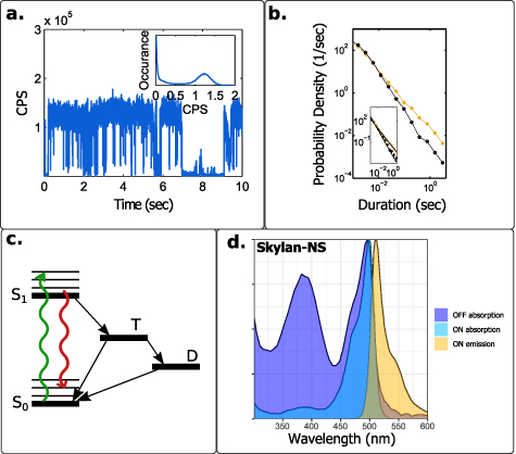
Figure 6. Fluctuations of common microscopy labels (a) intensity fluctuations in the fluorescence of a single QD. The emission is spontaneously interrupted by 'off' state periods. (b) State duration distributions for the 'on' (orange) and 'off' (black) states for the same QD shown in (a). QD blinking presents a power law distribution without a typical time scale. The inset shows fits to a power law function with −1.2 and −1.8 exponents for the 'on' and 'off' states, respectively. (c) A state diagram of a photoswitchable fluorescent dye. The molecule is excited with light (green) from the ground state S0 to the excited state S1. From there, emission (red) or crossing to the triplet state T and from there, a long-lived dark state D can occur. (d) Absorption and emission spectra of the photoswitchable Skylan-NS fluorescent protein [112] (adapted from [113]). Wavelengths in the 450–500 nm range can excite both dark and fluorescent states. Reprinted with permission from [105]. Copyright (2013) American Chemical Society.
Download figure:
Standard image High-resolution imageThe underlying mechanism of blinking remains an open scientific question. While some reports considered charging as the cause of dark periods [100], more recent works show that it is unlikely to be a universal explanation for blinking without a definite time scale [101–106]. For a thorough discussion of this topic we refer the reader to comprehensive reviews written on the subject [99, 107].
Currently, antibody conjugated CdSe/CdS core/shell QDs and similar variants are available commercially with a polymeric shell that reduces their toxicity for the sample and improves photostability (Qdot, Thermo Fischer Scientific). However, the generation of such well capped QDs results in relatively sizable objects with diameters of  10 nm, making it hard for them to penetrate the cell membrane and resulting in non-specific binding within cells [108]. In addition, their varying stability in solutions used for immunochemistry as well as inconsistent penetration depth present challenges for their use in biological research [109, 110]. As a result, while colloidal QDs present a high potential for SOFI and many other microscopy modalities they are still rarely used in such applications.
SOFI with fluorescent carbon nano dots have has also been recently demonstrated [111]. These organic nano particles are more suitable for organic labelling than their inorganic counterparts discussed above. Nonetheless, their relatively long 'off' states hinder the acquisition of higher-order SOFI images.
4.2. Fluorescent dyes
Fluorescent dyes are popular in bioimaging due to the enormous variability generated by proven synthetic routes, the wide availability of dye-conjugated stains, and the established sample preparation protocols. Dyes are organic molecules that emit light at a wavelength corresponding to the energy gap between ground and excited electronic states. In addition, they can undergo transitions to long-lived dark states that cause fluorescence intermittencies. These processes are strongly influenced by the interaction with the environment.
In a molecule illuminated with visible or ultraviolet light, an absorption transition occurs from the ground singlet electronic state with zero net spin (S0), to various vibrational levels in the singlet excited state (S1) (see figure 6(c)). Vibrational relaxation followed by relaxation to the ground state results in the emission of a photon within nanoseconds. Alternatively, an intersystem crossing to the triplet state with non-zero net spin can occur. Due to the spin selection rule, the triplet state relaxation to ground state is dipole-forbidden and therefore has a longer lifetime on the order of microseconds. The transition from the triplet excited state (T1) back to the ground electronic state is termed phosphorence. Alternatively, the molecules may progress to a second, long-lived dark state D, e.g. through a redox reaction [114] (see figure 6(c)). These states' lifetimes are strongly sensitive to their environment with durations of milliseconds to minutes. Such states are exploited in SMLM methods such as STORM to generate intermittent darkening.
An organic dye molecule in aqueous solution typically emits photons continuously until it is bleached with only short microsecond interruptions when the molecule inhibits a triplet state. Such interruptions are too fast for typical imaging experiments with framerates below 100 Hz. This relatively fast triplet-to-singlet relaxation is caused by dissolved oxygen from air that collides with dye molecules in the triplet state and repopulates their ground state. At the same time, these collisions produce singlet oxygen that is highly reactive and causes unwanted phenomena such as cellular damage [90].
In conventional microscopy, blinking is undesirable and the usual approach is to stabilise fluorescence using reagents that act as triplet state quenchers [90, 115]. On the other hand, for methods relying on stochastic switching, the goal is the opposite: generating dark states with long lifetimes. This is achieved by balancing the concentration of reducing and oxidizing agents, known as the reducing and oxidizing system. A detailed description of the chemical processes regulating photoswitching in dyes is beyond the scope of this review and can be found in [90]. Briefly, the blinking rate of dyes can be tuned by both the illumination intensity and chemical environment [114]. In SMLM methods, most emitters are kept in a long-lived dark state (D) at any given time in order to have less than one bright emitter within a PSF on average [7]. In contrast, fluctuation-based methods can deal with much higher emitter density per frame. For even-order SOFI cumulants, it can be shown that best contrast is achieved for on-to-off times ratio around 1/2 (see section 5.3.2). Note that unlike QD blinking, the switching times of dye molecules are distributed exponentially and a typical time can be mathematically defined [14].
By tuning the buffer composition, photoswitching from dark to bright states can be achieved in many types of dyes. Some of the most frequently used ones are cyanines such as Alexa Fluor 647 which was also the first organic dye demonstrated to be suitable for SOFI [116]. However, photoswitching of other classes of dyes such as rhodamines and oxazines has also been shown [90]. The abundance of photoswitchable dyes enables multicolor super-resolution imaging. In fact, SOFI can be applied to imaging of more channels simultaneously than conventional fluorescence microscopy [117]. By computing spectral cross-cumulants, additional virtual channels are generated and used for subsequent unmixing. Using this approach, simultaneous three-color imaging was demonstrated using only two physical acquisition channels.
Recently a new class of fluorescent dyes appeared, termed self-blinking dyes [118]. Although their blinking, stemming from a reaction called intramolecular spirocyclization, is still influenced by the microenvironment, it has been shown that the on-time ratio in standard buffers is already suitable for SOFI [119].
4.3. Fluorescent proteins
Fluorescent proteins (FPs) are especially attractive for bioimaging as they can be expressed in cells through genetic manipulation enabling labeling without the complex process of inserting dyes molecules through the cell membrane. Moreover, many FPs exhibit photoswitching whose rate is mostly sensitive to their structure as well as excitation wavelength and not the chemical environment as is the case for fluorescent dyes. A detailed discussion of the mechanism of this switching is beyond the scope of this paper and can be found, for example, in an extensive review of the photoinduced chemistry of FPs published a few years ago [120].
One of the best known reversibly photoswitchable proteins is Dronpa [121, 122], one of several green FPs derived from corals. Photoswitching from the dark back to the fluorescent state is achieved by illumination with UV light, although excitation of both fluorescent and dark state with one laser wavelength is possible (see figure 6(d)). Typical blinking dynamics of Dronpa under 488 nm excitation shows an exponential distribution of lifetimes with time constants in the range of tens of ms, with the exact value depending on the excitation power [121]. This means that the frame rate required to observe Dronpa blinking is well within the range of modern camera-based microscopes.
Other popular FPs that exhibit photoswitching are green fluorescent mEOS2 derivatives mEOS3.2, SkylanS and SkylanNS as well as red fluorescent mCherry. Of those, SkylanS [123] was developed specifically for SOFI. A systematic comparison of performance of 20 photoswitchable FPs at different imaging conditions along with the raw data can be found in [88, 124]. Out of the tested FPs, blue and cyan ones performed poorly, while green and red ones enabled a good SNR in second-order SOFI (in some cases with an additional UV illumination to assist with photoswitching). Notably, it has been shown that the green- and red-fluorescent photoswitchable proteins can be used together to achieve two-color or photochromic SOFI (pcSOFI) imaging [125].
4.4. Application of DNA-PAINT for SOFI
The usability of organic dyes and FPs for SOFI is limited by their inherent susceptibility to photobleaching. Glogger and coworkers presented an approach that circumvents this issue by using reversibly and transiently binding labels [126]. Based on PAINT and specifically DNA-PAINT [13], the method relies on fluctuations arising from attachment and detachment of fluorophore-labeled short DNA oligonucleotides to specific binding sites. These are labeled with target-specific antibodies containing complementary DNA structures. The probes are continuosly replenished from a buffer which serves as a reservoir, giving the method a highly sought-after immunity to photo bleaching. These labels are available commercially and have been used for SMLM as well as STED. Combining them with SOFI enables using shorter acquisition times through denser frames.
5. SOFI analysis: from raw data to a super-resolved image
In this section we will describe several aspects of reconstructing super-resolved SOFI images from raw data. First, we describe some issues arising during the application of the formulas given in section 2 to experimental data that is pixelated, finite in time and noisy. We briefly discuss the choice of experimental parameters and describe some of the main sources of artifacts arising from SOFI analysis and ways to circumvent them. Finally, we list available software packages for SOFI simulations and image reconstruction.
5.1. Image reconstruction
While the formulas given in section 2 are continuous in space and time, an image series acquired with a camera-based microscope consists of discrete pixels and frame acquisitions. The typical raw SOFI data consists of an image series of several hundreds or thousands of frames, reconstructed to obtain a single super-resolved frame.
For auto cumulants, processing a pixelated image series is straightforward: auto cumulants are calculated for each pixel independently with a time lag τ that takes integer values corresponding to a difference in frame number. Notably, since auto-correlations for  = 0 contain contributions from noise sources with short correlation times such as shot noise, they should be used with great caution for image reconstruction. Similarly, for higher-order auto-cumulants, the delays
  should be all different.
As evident from equations (2) and (3), any combination of non-zero and non-repeating delays (and any linear combination of such cumulants) would generate a super-resolved image with the same resolution. In general, a typical correlation function of blinking emitters decreases quickly with delay (see figure 7(a)), so selecting the shortest possible delay times leads to the highest level of correlation signal [127]. For long time delays, the effect of bleaching becomes apparent. Although at a first glance bleaching yields strong, noise-free SOFI images, it has been shown that the result does not correspond to the actual structure of the sample. Instead, cumulants computed for long time delays can be used to estimate the contribution of bleaching and if necessary, correct for it [89].

Figure 7. (a), (b) Dependence of SOFI signal on time lag and pixel distance, calculated from example experimental data with the SOFI evaluator [88]. (a) Average cross-cumulant signal depending on the time lag τ. Signal intensity quickly decreases to zero, indicating negligible bleaching contribution. (b) The cross-correlation for pixel pairs with different distance follows a Gaussian function. (c) Creating virtual pixels (blue) from correlations of camera pixels (black). All pixel pairs within a PSF (orange) diameter contribute to a virtual pixel in the middle. However, the exact number of pairs and pixel distances depend on the location of the new pixel (compare green and magenta).
Download figure:
Standard image High-resolution imageAlthough theoretically auto-cumulants offer the same resolution improvement as cross-cumulants, in practice, the resolution of an optical microscope is limited not only by PSF, but also by the camera pixel size. Therefore, it can be useful to calculate cross-cumulants in order to generate additional virtual pixels. An additional advantage is that by omitting the correlation of a pixel with itself, the above-mentioned effect of temporally-uncorrelated noise is avoided so that cross-cumulant can be computed for  , yielding higher SNR and simplifying the computation [41].
The principle of creating a virtual pixel by computing second-order cross-cumulants is shown in figure 7(c). To obtain a new pixel, pairs of opposite pixels are cross-correlated. It is apparent from the 'distance factor' in equation (4) that it only makes sense to include pairs up to one PSF width apart. Moreover, the distance factor serves as a weight for the contributions from pixel pairs with different distances and has to be divided by when combining different cross- and auto-cumulants into a single image, to avoid the so-called checkerboard pattern. If the PSF is known, calculating the distance factor is straightforward. Alternatively, considering the cross-cumulant of pixel pairs with different distances and assuming a Gaussian PSF, one can estimate the PSF width and use it for subsequent image reconstruction (see figure 7(b)) [41, 124]. The theoretical formalism for this analysis is outlined in [128]. Recently, a model-free approach to correct pixelation effect has also been demonstrated [129].
For higher-order cross cumulants the principle of computing virtual pixels is similar. The fluorescence signal from a set of n pixels can be used to create a new pixel in their geometrical center. However, one needs to keep in mind that an nth order cumulant contains contributions from correlations of all orders from 2 to n. The procedure of computing a cross-cumulant for a set of n pixels from correlations of its subsets is explained in detail in reference [130].
Finally, in a practical implementation of SOFI one must consider that correlations can occur from more banal sources than fluorescence fluctuations. A small drift or vibrations in the position of the stage, for example, will generate a signal that is proportional to the spatial derivative of the sample structure. Fluctuations in the illumination source power will also cause unwanted correlations. It is important to note that unlike correlation in emitters' fluorescence, such a signal would seldom contain any extra information that can be applied to super-resolution and is more likely to distort the SOFI image.
5.2. Choice of acquisition parameters
The theoretical concepts on which SOFI is based assume an infinite recording time. To obtain an image of a sample containing blinking emitters, a sufficiently long recording is required to for a trustworthy estimation of the average intensity of the emitters. Similarly, the cumulants require a sufficient frame number to converge toward their theoretical values.
The number of frames required for faithful image reconstruction depends on emitter statistics, that is, their blinking rate as compared to the acquisition frame rate and on-time ratio, emitter density and the noise level [46, 127, 131, 132]. Under good imaging conditions, second-order cumulants converge within a few hundred frames, corresponding to a few-seconds acquisition with a fast camera. For higher orders, this number grows quickly to a few thousand for the third and more than 10 000 frames required for the fourth order [127]. These order-of-magnitude estimates were obtained using numerical simulations and depend on the assumed imaging conditions and the exact data analysis procedure used for SOFI. The dependence of acquisition time on the order of cumulant is a complicated topic and it is difficult to provide clear and general guidelines. This issue is further complicated in a real experimental setting due to fluorescence bleaching, sample drift and similar factors. Various ways for noise filtering of the raw image stack have been proposed to decrease the frame number [133] or increase the cumulant order that can be computed for a given frame number [134], but have not been widely applied yet. Data pre-processing can also be used to correct for photobleaching artifacts and as a result improve the contrast of SOFI images [135].
In conventional microscopy, longer exposure times and higher illumination intensities yield a higher SNR. At the same time, for SOFI, the frame exposure duration has to be short enough to register blinking. The optimal exposure time will be a trade-off between these two factors. Similarly, illumination intensity should be chosen so that it does not cause bleaching or damage the sample during the long recording.
5.3. Artifacts in SOFI images
5.3.1. Non-linearity and balanced SOFI
In theory, going to higher orders in the SOFI analysis reconstructs the imaged sample with an increasing resolution. In practice, however, with increasing order, the super-resolved image may become more distorted due to a growing presence of artifacts. Here we will discuss two main issues: the non-linear dependence of SOFI contrast on emitter brightness as well as so-called cusp artifacts.
In the expression for the nth-order cumulant (equation (3)), it is not only the PSF  that is raised to the power of n but also the molecular brightness,
  . Its heterogeneity will therefore be amplified in the generated super-resolved image. As a result, emitters that are only somewhat dimmer in the averaged image may be hardly distinguishable in a high-order SOFI image.
A simple approach to non-linearity compensation is local dynamic range compression (ldrc) [130]. In ldrc, the dynamic range of the pixel intensities of a high-order SOFI image is compressed in a local manner to that of a lower resolution reference image (e.g. the 2nd-order SOFI image). For this, a small moving window is defined, and the pixel intensities within the window are rescaled to the intensity range of the same area in the reference image. The window is then moved across the field of view and the output image with compressed dynamic range is formed by the average of all the rescaled windows. The reference image is usually the 2nd-order SOFI image that has good background removal and only moderate dynamic range expansion.
A more complex analytical approach called balanced SOFI has been proposed in reference [136]. The authors point out that cumulants of different orders calculated for the same raw data form a system of equations that can be locally solved for the independent variables molecular brightness, density and on-time ratio. This can be used to reconstruct a super-resolved image with linear brightness response. In the paper, the authors compare 5th-order balanced cumulant with 5th-order SOFI, where the dynamic range is too high to be represented meaningfully. In contrast, the bSOFI image is nearly linear in brightness. In addition, balanced SOFI can give extra quantitative information about the emitters themselves (see sub-section 8.2). It should be noted, however, that the spatial resolution of the estimates of these calculated parameters is limited by the lowest order cumulant used in the linear combination.
While a suitable linear combination of cumulants of different orders provides a solution to the dynamic range issue, it is not an entirely analytical one. Each order yields a different resolution and SNR, so that their combinations will potentially generate different artifacts and have limited resolution improvement. To overcome this issue, deconvolution is performed before calculating the linear combinations, which is also a limitation of the method: since deconvolution is highly sensitive to noise, bSOFI reconstruction may not be possible for images with low SNR. In that sense, bSOFI can be constructed as a one of the first fluctuation contrast reconstruction algorithms that appeared in recent years (more on this in section 6).
5.3.2. Cusp artifacts
Another issue that limits the use of higher cumulant orders is the sign dependence of cumulants, of order three and higher, on the emitter blinking statistics. This was first described in detail by Yi and Weiss [137] and termed a cusp artifact.
The time that an emitter spends in bright and dark states depends on emitter's properties and its environment, including factors such as local chemical environment, emitter orientation, proximity to other fluorophores or local excitation power. Moreover, all fluorophores experience bleaching which is equivalent to permanently staying in a dark state. The impact of the switching statistics on the SOFI image can be understood by looking at equation (3) and assuming that an emitter switches only between two states, 'on' and 'off'. Then, if ρ is the on-time ratio, the emitter's nth order cumulant is proportional to an nth degree polynomial  [137]. The first five ωn
polynomials are shown in figure 8(a). Naturally, all polynomials reach zero for ρ equal to 0 or 1, corresponding to an emitter permanently remaining in the same state, i.e. not blinking. Importantly, while the second-order cumulant is always positive, higher-order cumulants take both positive and negative values. If the value of ρ could be well controlled for all emitters this would only result in a constant multiplication factor. However, given the number of factors influencing the fluctuation statistics, this is typically difficult to achieve. As a result, the varying contrast sign can severely distort the SOFI image.
[137]. The first five ωn
polynomials are shown in figure 8(a). Naturally, all polynomials reach zero for ρ equal to 0 or 1, corresponding to an emitter permanently remaining in the same state, i.e. not blinking. Importantly, while the second-order cumulant is always positive, higher-order cumulants take both positive and negative values. If the value of ρ could be well controlled for all emitters this would only result in a constant multiplication factor. However, given the number of factors influencing the fluctuation statistics, this is typically difficult to achieve. As a result, the varying contrast sign can severely distort the SOFI image.

Figure 8. The cusp artifacts effect. (a) Dependence of polynomials  on the on-time ratio ρ. (b)–(d) SOFI image showing 3 nearby fluorophores. In (b) each emitter has the same on-time ratio. In (c) the cumulant value of the middle emitter has an opposite sign compared to the others. (d) presents the situation when all emitters have different cumulant values and signs, the most realistic scenario. (e) Simulation of SOFI images of orders 2nd to 5th for different bleaching and noise levels (reproduced from [137]. CC BY 4.0.). First row: no noise or bleaching. Middle row: bleaching added. The image can still be reconstructed. Lower row: even a low amount of noise degrades the higher-orders images so that the sample features are hardly recognisable.
Download figure:
Standard image High-resolution imageSimplified simulations shown in figures 8(b)–(e) illustrate how the change of cumulant sign leads to artifacts. A simple simulated image of three emitters is shown in figures 8(b)–(d). First, emitters with identical properties present an artifact-free image (figure 8(b)). In the next panel, we assign a negative sign cumulant to one of the emitters resulting in dark boundaries between the positive and negative areas, which are the origin of the term 'cusp'. In the bottom panel, the emitters have different cumulant amplitudes, as well. Importantly, each such combination leads to a substantially different image, showing how difficult it is to interpret higher order SOFI images. Finally, figure 8(e) adapted from [137] shows a more realistic simulation that includes multiple emitters as well as noise and bleaching. As soon as a low amount of noise is introduced, in combination with the cusp artifact, it degrades higher order cumulants to such an extent that no image can be reconstructed beyond the second order.
In another paper Yi and co-workers propose a solution to circumvent cusp artifacts [130]. Their approach is to reconstruct the image using statistical moments instead of cumulants. In contrast to cumulants, even order moments do not exhibit sign change. However, this solution entails a problem, since moments of order higher than 2, contrary to cumulants, do not eliminate cross-terms coming from multiple emitters and therefore do not, as such, produce a super-resolved image (see section 2.2.1). As a result, the cross-terms limit the resolution enhancement to a factor of  . To overcome this issue, deconvolution algorithms can be applied to even-order moments. The authors claim that this enhances the resolution further, leading to a total improvement by up to a factor of
  (compared to n in the case of deconvolved SOFI). In the paper, super-resolution image reconstruction from live-cell-imaging data up to the 6th order is shown and compares favorably to other methods, including bSOFI.
5.4. Available software packages
While the lowest order auto-cumulant is straightforward to compute in any programming language, the implementation of higher order auto- and especially cross-cumulants is much more involving. Furthermore, increasing the cumulant order also increases the number of pixel and time lag combinations to include in the computation. This means that carefully written code using efficient dedicated libraries becomes more important. A good starting point is to use existing packages which will be briefly described here.
Localizer is a package for super-resolution microscopy image analysis created by Dedecker and co-workers [138]. It offers the option to calculate SOFI cross-cumulants of orders up to 6 with many available options regarding, for example, the number of pixel combinations included (where the default is calculating the cumulant only between pairs of closest pixels). Localizer is written in C++. A GUI version is provided in the form of a plugin for Igor Pro (WaveMetrics, Inc.). A Matlab MEX file is also available.
Recently, another Igor Pro plugin that based on Localizer has been published. SOFIevaluator [88] is a tool that analyses a raw image by calculating a set of metrics describing the quality of data for the purpose of SOFI analysis, such as the SOFI SNR and the magnitude of bleaching. It can be used to quantitatively compare different fluorophores and parameters for image acquisition in order to select the best imaging conditions for a given experiment.
For bSOFI [136], a MATLAB toolbox has been developed for two and three-dimensional SOFI analysis [139]. It allows to reconstruct the image using third and fourth-order cumulants.
A simulation tool has been developed to test the influence of different factors on the outcome of super-resolution reconstruction [140]. The package includes simulation of SOFI cross-cumulants of different orders, as well as bSOFI. Moreover, it allows to compare SOFI reconstruction to STORM. Its purspose is to get an idea of what imaging conditions would lead to a successful analysis before running an experiment. It can be also a learning tool, since the processing steps of SOFI are visualized and explained in a tutorial-like way.
6. An algorithmic approach to fluctuation contrast microscopy
The topics and developments described in section 5 are extensions to the analysis in the original SOFI demonstration [22]. As such, they provide analysis recipes that can be written in closed-form, i.e. one can write the mathematical expression for the super-resolved image and directly observe the resolution improvement (e.g. narrowing of the PSF). This section describes a more general approach in which an image can be reconstructed from the raw data of fluorescence fluctuations through an optimization algorithm. While such a method is more 'elusive' and one cannot directly determine how well will it work for a particular measurement, it offers the integration of different types of prior information that we have on the sample structure and the imaging system. Such extra information can be valuable for reconstructing the sample structure.
SOFI and related methods rely on spatio-temporal correlations in the fluctuations within a set of images. More generally, exploiting fluctuations is probably the most successful approach to super-resolution imaging, including the most widely used set of super-resolution methods, SMLM (e.g. STORM and PALM). In SMLM, only a small fraction of labels contributes to each frame, generating a very sparse scene (typically below 1 µm−2). Successive pinpointing of the emitters' positions in each frame generates a super-resolved image within about a thousand frames.
In contrast, the raw data collected in SOFI contains considerably denser frames in which a substantial proportion of the total number of emitters is in a fluorescent state. As a result, such frames are an obvious candidate to achieve super-resolution microscopy without the burden of lengthy acquisition times associated with SMLM. However, the original, straightforward SOFI analysis as introduced in section 2 produces only a modest resolution improvement within a few seconds of exposure time. Unlocking the full potential of this type of complicated data which includes many emitters with randomly fluctuating intensities is a task more suitable for optimization algorithms.
In the following subsections, we explore the algorithmic reconstruction of images with an increasing level of density and complexity. The diagram in figure 9 presents a summary of the different types of methods (black text) with notable examples (red text) and the appropriate section number in this review (purple text). First, section 6.1 describes the extension of SMLM to localization of overlapping emitters. The success of these techniques inspired researchers to go a step further and reconstruct images of denser frames without a localization fit approach, as described in section 6.2. Finally, section 6.3 reports on the growing activity in interpreting very high density frames with the application of deep-learning methods.

Figure 9. A diagram presenting the different algorithmic approaches introduced in section 6 and some specific example for each approach (red text). The original demonstrations of STORM and PALM used fitting algorithms classified here as single-emitter localization methods. The maximal interpretable frame emitter densities were 0.01–0.1 µm−2. Applying frames of higher densities required an algorithm from the multi-emitter localization family such as DAOSTROM and CSSTORM. Since their performance is significantly reduced at >1 μm−2, more sophisticated image reconstruction techniques were developed. For example, SPARCOM, MUSICAL and SRRF. Finally, very recently, deep-learning methods were successfully applied to fluctuating-emitters raw data, demonstrating reconstructions from frame densities of  and even beyond.
Download figure:
Standard image High-resolution image6.1. Tackling overlapping emitters in localization microscopy
The initial breakthrough demonstrations of SMLM used sparse frames with well-separated emitters, thus avoiding the risk of overlapping PSFs [6, 7]. The result was a trade-off between superb resolution and a prohibitively long acquisition time of a few hours. Even though improvements in emitter brightness and switching times reduced the total exposure time, the low density of each frame was the obvious main hurdle for live-cell imaging. As a result, within a few years initial attempts to algorithmically analyze images of overlapping emitters emerged [73, 141, 142]. While single emitter localization methods failed to efficiently process raw frames with >1 μm−2 emitter densities, methods such as DAOSTORM and CSSTORM where able to analyze fairly well frame densities of up to 5–10 µm−2 [141, 142]. Accordingly, the acquisition time was reduced by an order of magnitude to a few seconds per super-resolved frame [143].
From an algorithmic point of view we can divide these methods into two groups. In the first, an iterative process locates bright emitters (and groups) and removes them from the image in order to find the residual emitter locations [141]. The success of such an approach critically depends on precisely characterizing and modeling of the experimental PSF [73]. In addition, such multi-emitter localization procedures are computationally demanding.
The second group of algorithms is based on compressed sensing. Generally, a reconstruction algorithm attempts to minimize a positive-valued 'cost function' which approaches zero when the fit matches the experimental data. A common example of such a function is the sum of squared differences between image and model (squared errors) over all pixels. Whereas the previous algorithm group attempted to minimize only the sum of squared errors, a compressed sensing algorithm also imposes sparsity. That is, the cost function increases with the use of more emitters to reconstruct the image. This approach avoids over-fitting of the noise patterns with many emitters and applies sparsity of frames as extra information.
Both algorithmic families have developed over the past decade and already include many sub-methods and software packages available for users. A comparison of their performance is an incredibly intricate task which is tackled for example by the Super-resolution fight-club competition [20, 21]. The quality of analysis method can be measured by multiple metrics (localization rate, false positives, false negatives, localization accuracy etc) and will depend on the emitter density, SNR and sample structure (2D vs. 3D, lines vs. areas etc) in a specific experiment.
Finally, it is instructive to note that these methods are developed with the conditions of SMLM experiments in mind. Thus, they typically include only a minimal consideration for the time domain and treat subsequent frames as independent. An exception are methods that identify emitters that appear in multiple consecutive frames and average their localization position (temporal grouping) [21, 144]. However, a recorded image series of fluctuating emitters contains much more information in the temporal domain that localization reconstructions tend to overlook. For example, emitters are typically active in a few different periods along the acquisition time. The following section introduces computational microscopy methods that make use of both the temporal and the spatial information in the raw data. With this combination they aim to reconstruct frames with a higher density of emitters and thus provide super-resolved images at a higher frame rate.
6.2. Image reconstruction for high density frames
Whereas the above-mentioned computational imaging techniques were conceived with the raw data of SMLM in mind, recently a lot of attention was devoted to methods for reconstructing super-resolved images from SOFI-like data sets. That is, analyze dense frames in which emitters rapidly switch back and forth between the bright and dark states. Containing far more emitters, such dense frames have the potential to produce a faster super-resolved reconstruction of a sample. We emphasize here that the above-mentioned change from SMLM to SOFI-like data requires a conceptual shift. In the latter, information about the sample structure is stochastically spread over the time series and extracting it is a convoluted task.
Before we approach methods that, like the original SOFI analysis, make direct use of auto- and cross-correlations, we describe two techniques that address fluctuations differently. The first, multiple signal classification algorithm (MUSICAL) uses singular value decomposition (SVD) to decompose an image stack to orthogonal components [145]. After reshaping the image stack into a 2D matrix with one dimension for time and the other for all pixels, SVD decomposes the stack into a sum of components, each of which is a product of a temporal and spatial vector. A weight factor determines their level of contribution to the image stack intensity. One can then attempt to separate signal from noise components and calculate a so-called indicator function pointing to the location of the emitters.
A second strategy to decompose the fluorescence fluctuation image stack is adopted by the Haar wavelet kernel (HAWK) analysis [18]. Data from emitters that partially overlap in time and space, are separated by considering the length and frequency of blinking events. This generates a substantially longer data set, increasing the level of sparsity in the data. Applying an additional algorithm, such as multi-emitter localization produces the super-resolved image. In fact, a SOFI or b-SOFI analysis combined with a HAWK pre-processing can be advantageous in avoiding non-uniform illumination artifacts [146].
A few computational imaging methods come even closer to the original concept of SOFI, incorporating temporal correlations. A notable example is sparsity-based super-resolution correlation microscopy (SPARCOM) [23]. In SPARCOM, the concept of signal sparsity is applied to the pair-wise correlation of all pixels in the image. Assuming that emitters fluctuate independently, the correlation signal is even more sparse than the original image stack, with non-zero values centered only around the diagonal. As a result, a sparse reconstruction of the signal can perform well up to higher frame densities. According to simulations SPARCOM analyzes scenes with >10 μm−2 emitter density with less than  false positive localizations. Similar approaches were recently used to reconstruct images from the quantum [147] and fluctuations where images of Q-ISM and ISM were merged using a sparsity reconstruction to generate super-resolved images at a few millisecond per pixel exposure. Following this line, a recent report from the same groups performed reconstruction of SOFISM data sets (see section 3.1.3), showing that reconstructing the entire scan image stack can outperform pixel reassignment in terms of resolution [148].
A non-optimization approach to correlations signal is taken in super-resolution radial fluctuation (SRRF) microscopy [149]. In SRRF, each frame is transformed into a radiality map, a non-linear transformation which heightens sample features in which the intensity gradient point to a an origin. A temporal correlation of a radiality stack yields a super-resolved reconstruction for densities in which multi-emitter localization algorithms fail. A promising demonstration of SRRF showed fixed-cell super-resolved images at a 1 Hz frame rate [150]. A recent comprehensive comparative study, however, found substantial discrepancies between SRRF reconstructions and the ground truth object, especially in non line-like features [19], while another study by Yi et. al have found that SRRF achieved a very high resolution at the expense of distorting some features and in particular artificially narrowing line features. We note that while SRRF generate a clever non-linear transformation of the SOFI data, it does not provide any extra information temporally or spatially and is therefore not expected to perform well as other method described in this section.
Finally, we review the method of entropy-based super-resolution imaging (ESI) [151]. Its analysis requires the computation of Shannon information weighted temporal-correlations. Although the correlation orders are differently classified in ESI it seems that it produces a similar resolution to the original SOFI analysis.
6.3. Fluctuation-based super-resolution via deep-learning algorithms
In recent years, deep learning techniques have been applied to the most challenging tasks in science and engineering including the fundamental limits of optical microscopy [152–154]. The hope of advancing far-field super-resolution microscopy drove a lot of attention to the application of deep learning techniques to analyze the standard data sets measured for SMLM and SOFI [24, 155, 156]. In this sub-section we provide a few examples of such attempts and briefly discuss the potential and risks involved in deep learning for super-resolution microscopy.
Briefly, a neural network algorithm can be thought of as multiple layers in which a linear manipulation of the raw data is followed by a non-linear step that zeros lower values. The parameters for the linear operations in each layer are optimized in the training phase where a ground truth dataset is compared with the output of the network. After training, the network is ready to tackle a similar analysis for previously unseen data.
In a similar spirit to the works presented in section 6, the basic challenge in the works described below is achieving SMLM-level super-resolution within more reasonable acquisition times. One approach, termed ANNA-PALM, attempts to do so by training a network to recognize structures according to under-sampled SMLM data [155]. The network is trained to reconstruct an super-resolved SMLM image, generated from a large number of low-density frames, from a small subset of frames. Impressively, for simulated data, the network achieves a similar quality of reconstruction as SMLM for roughly  less frames. Experimental images of micro-tubules within fixed-cells, that agree with the SMLM ground-truth, were obtained from just tens of frames with an overall exposure time of
  1 s. However, such an approach is very specific to the type of sample for which the network is trained. In essence, in the lack of sufficient localization to sample a super-resolved image (sampling below the Nyquist rate), the network completes the image with patterns that are most similar to those that it was trained on.
To avoid such a risky sensitivity to sample type caused by under-sampling, Deep-STORM attempts to improve the analysis of dense frames containing plenty of information [24]. Here, the network simply tries to outperform the previous multi-emitter localization algorithms in finding positions of overlapping emitters. Training with images of sparse in-vitro blinking QDs, the authors successfully reconstruct images of micro-tubules labeled with the same QDs. In the context of this work, we note that one common advantage of neural network solutions is the ability to reconstruct images without user-tuned parameters, a process that is time consuming and requires a lot of expertise. In a more recent work from the same groups, the authors show very good results in reconstructing 3D SMLM data [157]. They combine deep learning with a PSF engineering approach: the 3D PSF of the microscope is adjusted to a so-called Tetrapod, shown to contain a higher level of information on the 3D location of a point emitter [9]. Analyzing the images with such a PSF, a convolutional network obtains 3D super-resolution images even in relatively high emitter densities. An exciting approach examined in this work is the optimization of the optical system itself (PSF engineering) together with the encoding deep neural network. Through simulations, the network 'discovers' a new optimal PSF that is better behaved than the result of a previous numerical optimization, the Tetrapod function, in high-density localization.
The final approach we review here is termed LSPARCOM and is based on the classical sparsity-based SPARCOM algorithm, introduced in section 6.2. This network shows two advantages over the two previous implementations: its is less sensitive to experimental parameters such as the sample structure redundancies (like ANNA-PALM) or the imaging parameters (like DeepSTORM) and it uses a less deep and more interpretable network [156]. In fact, the authors claim that the first property is the result of the second; using a small number of training parameters does not allow the network to learn training-set specific feature of either the sample or the optical setup. Such flexibility can be very helpful for experimental applications where the PSF itself, for example, can depend on the sample through scattering and refractive index.
Naturally, when observing the results of neural networks in super-resolution a word of caution is in place. Like for other algorithms, it is difficult to ascertain that the reconstruction is indeed trustworthy; however, as so-eloquently phrased in [154] deep networks are 'specifically trained to lie plausibly'. That is, they are trained to use among others the structural redundancies in their training sets in order to extend the amount of information stored in the data. It is therefore re-assuring to note that DeepSTORM can be trained on randomly positioned emitters and performs very well on cell-like simulations and experimental biological samples. LSPARCOM presented in-part such flexibility by training on different types of simulations, but it seems that all training and data samples included line feature with intersections.
6.4. Evaluating algorithmic reconstructions
While the description of the different algorithmic approaches in this section focused mainly on their potential for super-resolution microscopy, we note that valid concern is often raised with regard to the use of reconstruction algorithms. Unlike most of the early demonstrations of super-resolution microscopy (e.g. SMLM, STED, SOFI, SIM and ISM) algorithmic reconstruction, by nature of being an optimization problem, is not based on a closed-form mathematical model. When such a model is not present we cannot be assured that a super-resolved image truly represents the object, even under proper experimental conditions. Whereas, for example, a SOFI image under poor experimental condition appears naturally noisy and difficult to interpret, an algorithmic reconstruction may appear completely clear with features that do not reflect the structure of the object whatsoever.
Since most of the methods described above have been introduced within the past 5 years, it is certainly too early to firmly state in which situation a specific method is useful. As external observers, we believe that an impartial testing grounds for different algorithms under various conditions (simulated and experimental), akin to the super-resolution fight-club [21], is critically important for the progress of this field. Although many of the works cited here follow the high standard of comparing themselves to multiple other algorithms, we feel that the level of expertise in operating these complex methods is not equal and generates bias in such comparisons.
7. Quantum correlation imaging
The combination of imaging and quantum optics has been explored since the early experiments with entangled photon pairs [158]. Typically in a quantum imaging experiment one generates a quantum state of light in a dedicated setup, uses it to illuminate the sample and measures correlations in light that interacted with the sample.
These standard quantum imaging methods are limited by the fact that delicate quantum correlations are difficult to maintain in a biological sample, because entangled states are susceptible to loss. Such methods relying on quantum entanglement have not yet been successfully applied to biological super-resolution microscopy.
An entirely different approach to quantum imaging has been proposed by Schwartz and Oron [159], who realized that most of the labels commonly used in fluorescence microscopy are actually sources of 'missing photon pairs', which can be used to break the diffraction barrier. This observation implies that all the microscopists working with fluorescent dyes, FPs or QDs are routinely generating quantum states of lights. Even more strikingly, the labeled biological sample itself is the source of quantum light. The quantum properties of fluorescence light can be revealed and used when standard intensity measurements are replaced with photon correlation measurements.
The super-resolution microscopy methods described in this section can be viewed as quantum analogs of SOFI in which the origin of correlations is not the classical intensity fluctuation, but the single photon emission of fluorophores.
7.1. Quantum correlations
Intensity correlation measurements of light, now the cornerstone of quantum optics [160, 161], were first investigated in the context of astronomy [162]. In their seminal experiment, Hanbury-Brown and Twiss analyzed a setup in which light is split at a beam splitter and falls onto two photodetectors [163]. This setup is schematically represented in figure 10. The intensities measured by the two photodetectors are correlated. The intensity correlation is typically plotted as a function of time delay (see the bottom part of figure 10). For thermal light sources, intensities measured by the two detectors are positively correlated at small temporal delays as a consequence of the fluctuations of the emitted light intensity. This tendency of photons from a fluctuating source to be detected together is called bunching. Single photon emitters, in turn, exhibit an intensity anti-correlation at small delays, a phenomenon dubbed antibunching (see figure 10(a)). This is a consequence of the fact that a single emitter can emit at most one photon at a time. Antibunching, observed for the first time in the fluorescence of atoms in 1977 [164], is one of the first experiments that can only be explained in terms of a quantum theory of light [165]; it can also be considered as the first experimental proof for the existence of photons.

Figure 10. The concept of Hanbury Brown Twiss setup used to detect quantum and classical intensity correlations. The experimental setup consists of a beam splitter and two detectors followed by time tagging electronics. (a) Antibunching—intensity anti-correlations. A cartoon representing light from a single photon emitter and the corresponding results, a dip at the zero delay time in the second order correlation function. The dip's width corresponds to the fluorescence lifetime (nanosecond timescale). (b) Blinking—positive intensity correlations. A cartoon representing the light from a fluctuating source and the corresponding second order correlation function which has a peak around the zero delay with a width governed by the rate of blinking. The typical time scale at which we observe blinking is on the order of milliseconds.
Download figure:
Standard image High-resolution image7.2. Super-resolution imaging with quantum emitters
The idea to use photon pair detection in a fluorescence microscope to achieve super-resolution has been introduced by Hell et al [166]. It remained impractical because of the lack of fluorescent two-photon emitters until Schwartz and Oron noticed that every single photon emitter can be considered a source of missing photon pairs [159] (the idea explained in more detail below). Soon after their proposal, the idea has been experimentally realized with QDs [3] and Nitrogen-Vacancy centers [167]. In fact, most emitters used in fluorescence microscopy, including fluorescent dyes [168] and proteins [169] as well as QDs [170], are single-photon sources. As a result, they can be used as labels for antibunching microscopy.
Antibunching is a single-emitter phenomenon in the sense that a single-photon emitter, such as a dye molecule, can only emit one photon after it is excited and then needs to be re-excited before it emits again. This does not mean, however, that antibunching cannot be observed when more than one emitter is present in the observation region. In such a case there are still less photon pairs emitted simultaneously than at a non-zero delay, and we observe a dip, though not a zero value, of the second-order correlation function at zero delay. The area of this dip, representing the number of missing photon pairs, is the antibunching microscopy contrast.
Antibunching-based imaging was first demonstrated in a wide-field microscope which required an ingenuous experimental setup with pulsed excitation frequency-matched to the frame rate of an EMCCD camera. Working at the kilohertz rate resulted in long acquisition times, limiting the practical applicability of the method [3]. The other demonstration that used nitrogen-vacancy centers [167] was performed in a confocal setup with fast detectors. NV centers offer excellent photo-stability, but are rarely used for fluorescent bioimaging. These approaches had to be further developed to go beyond a proof-of-concept demonstrations.
Recently, quantum antibunching microscopy has been combined with another super-resolution microscopy technique, namely ISM [58–60] (introduced in section 3.1.3). This combination is termed Q-ISM [25]. This followed a theoretical proposal for a wide-field variant, combining quantum correlations and SIM, by Classen et al [63]. They found that, theoretically, the resolution improvement factor surpasses the one obtained by each method separately. Q-ISM was used to obtain super-resolved images of a microtubule sample labeled with QDs. Figure 11 compares performance of Q-ISM to that of CLSM and classical ISM on the same data set collected by an ultrafast camera composed of a fiber bundle connected to single photon avalanche diodes (see subsection 3.1.3). A CLSM image (figure 11(a)) is obtained by adding the count rates collected by different detectors at each step of the scan, whereas for ISM (figures 11(b) and (c)), images acquired by the individual detectors are shifted prior to addition.
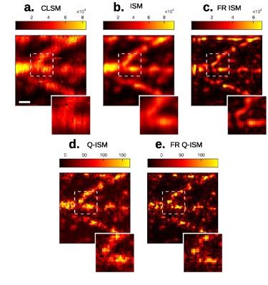
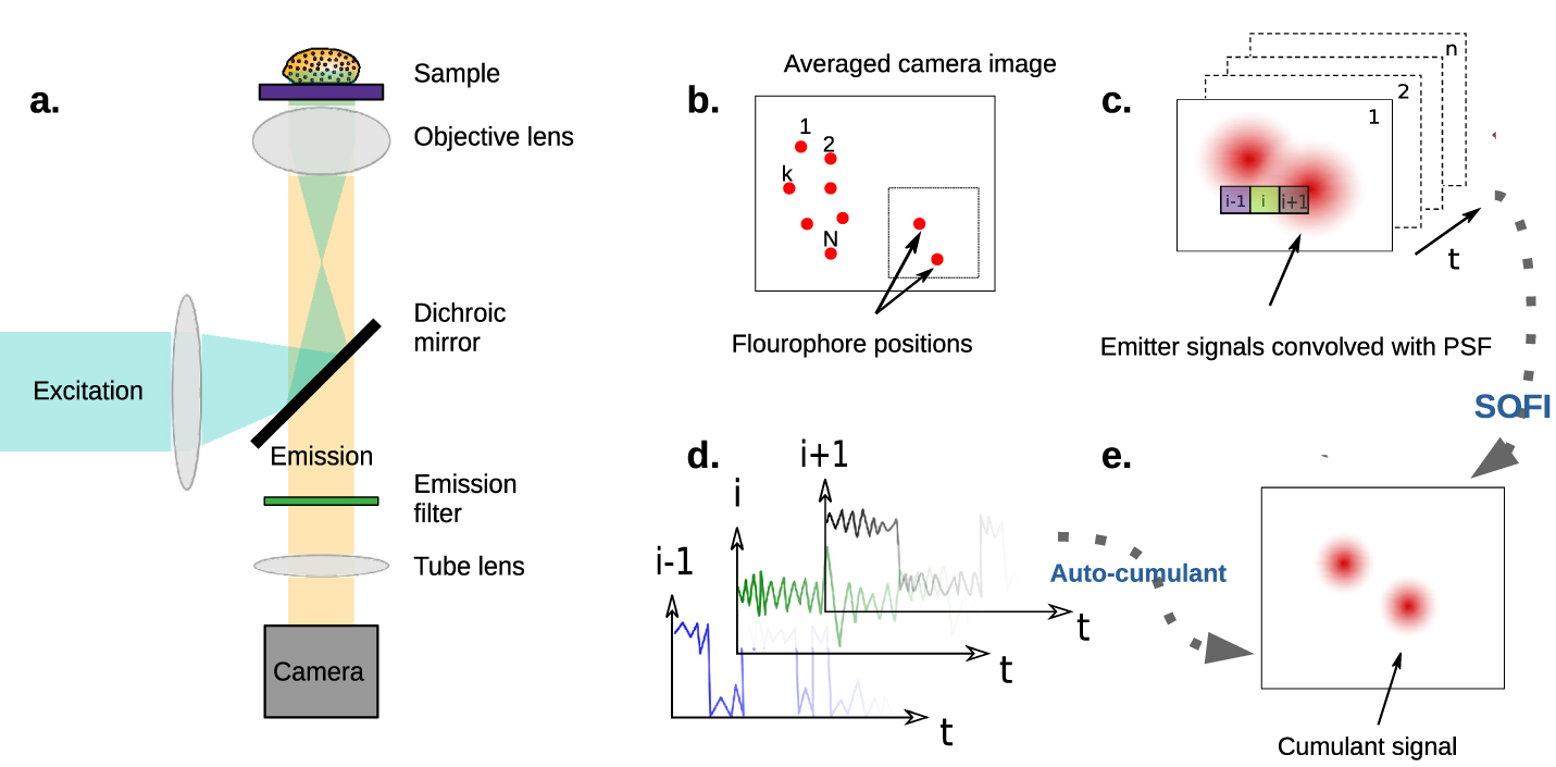
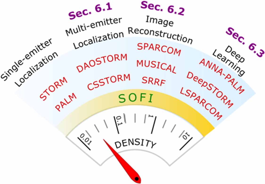
Figure 11. Quantum image scanning microscopy (Q-ISM) of microtubule cell samples labeled with quantum dots: (a) confocal laser scanning microscopy (CLSM) image, (b) image scanning microscopy (ISM) image, (c) Fourier re-weighted (FR) ISM image, (d) Q-ISM image, and (e) FR Q-ISM image. All images were analyzed from a confocal scan (50 nm steps, 100 ms pixel dwell time) of a 3 µm × 3 µm section of microtubules in a fixed 3T3 cell labeled with fluorescent quantum dots (QDot 625, Thermo Fisher). Scale bar: 0.5 µm. Figure and caption adapted from [25].
Download figure:
Standard image High-resolution image
It can be observed in figure 11 that Q-ISM features higher resolution than ISM. Unfortunately, because of losses and non-unity QEs of fluorescence emission and detection, the detected number of missing photon pairs is substantially smaller than that of overall photons. As a result, Q-ISM suffers from a smaller SNR compared to ISM. One should keep in mind that the Q-ISM signal is recorded together with the ISM signal and therefore it seems natural to combine the information present in the two signals. This can be achieved algorithmically, for example by using joint sparse recovery methods as demonstrated in [147].
First demonstrations of antibunching microscopy relied on avalanche photodiodes for confocal modality and EMCCD cameras for wide-field modality. EMCCD cameras offer a high number of pixels and an excellent QE, but are slow (see section 3.2.1). In [171] an ultrafast 'camera' was built using a fiber bundle, multiple SPADs, and a time-tagging unit. Each pixel in this camera was capable of timing detection at sub-nanosecond resolution, but the number of pixels was quite limited. The emerging technology of SPAD arrays offers a promising avenue for antibunching microscopy in confocal [86] and wide-field modalities (see section 3.2.2). Antibunching microscopy can be considered to be a quantum analog of SOFI and as a result can be described by an analogous theory leading to the same PSF functions as standard SOFI. Nevertheless, the physical phenomena underlying the correlations are entirely different. In the case of standard SOFI the correlations result from emitter blinking, whereas antibunching, a genuinely quantum phenomenon which marks the reduction of fluctuations (sub-Poissonian statistics) is the source of correlations in quantum SOFI (see figure 10). This fundamental difference between the two techniques bears practical implications that we will describe in the following section.
7.3. Blinking and antibunching: differences and their consequences
Blinking statistics and dynamics depend heavily on the chemical micro-environment and the excitation power (see section 4) and as a consequence the contrast of SOFI microscopy carries additional information about these factors, but at the same time it is prone to artifacts. In contrast to blinking, antibunching is independent of the above mentioned factors and used as a microscopy contrast is less prone to artifacts. Many fluctuations can result in positive correlations which will generate an artificial contrast e.g. laser power fluctuations or stage position oscillations, but it is much less common to generate false negative correlations through technical imperfections.
The time scales of blinking and antibunching are different. Antibunching is governed by the fluorescence lifetime which lies in the nanosecond range, whereas blinking typically occurs at the timescale of microseconds up to seconds. For continuous excitation, the requirement for antibunching microscopy is to resolve detections at a resolution below the fluorescence lifetime, which is technically challenging. This issue can be circumvented with the use of pulsed excitation, as long the pulse duration is much shorter than the fluorescence lifetime [3, 25]. While there are exceptions, typically photon counting detectors (Geiger mode), are used in quantum correlation SOFI [86], whereas the implementation of classical SOFI is simpler since it can be conveniently measured with slower detectors such as standard cameras.
7.4. Emitter counting by quantum correlations
Measurements of quantum correlations can be also used to count emitters within a diffraction-limited spot of a confocal laser scanning fluorescence microscope [172–176]. This is analogous to bSOFI (described in section 5.3) which can extract the information about emitter properties from a combination of different correlation orders [136]. It is quite intuitive that the antibunching contrast carries information about the number of emitters within the observed spot. If the normalized second order correlation function,  , is close to zero, we infer that we are observing a single emitter, for a high number of emitters
  approaches 1. Generally,

where M is the number of active emitters within the observed spot with an equal intensity of emission. As can be seen from expression (8), emitter counting using the value of  can work reliably for a small number of emitters. Recording multi-photon statistics (higher order correlations) enables inferring the emitter number with precision of a few percent even for tens of emitters [172]. Studies performed in the Herten group demonstrated the feasibility of emitter counting based on photon statistics for various fluorescent dyes [173]. A systematic comparison of performance of dyes in this technique is given in [176]. In [177] molecule counting by photon statistics has been implemented within a confocal microscope. This enabled the authors to obtain maps containing the number of molecules contained in sub-diffraction regions.
Emitter counting by photon statistics can be used to enhance super-resolution microscopy. It has been combined with STED microscopy [177] and used to speed up data acquisition in a proof-of-concept localization microscopy measurement [171]. Israel et al have demonstrated that  measurements can be used to aid fast localization microscopy [171]. The speed of localization microscopy is typically limited by the requirement for emitters not to overlap spatially within any frame (see section 6). The information about the number of active emitters within the diffraction limited spot obtained from
  measurements allowed Israel et al to filter-out the unwanted frames with multiple active emitters.
8. Selected biological implementations
8.1. Live-cell imaging
Although SOFI for bioimaging was first demonstrated more than 10 years ago [22], it remains significantly less popular than SMLM, most likely because of the modest resolution improvement it typically offers. However, the need to reduce acquisition time and illumination intensity in live-cell imaging makes it challenging to use SMLM. SOFI performs better than SMLM at low SNRs and is applicable over a wider range of labeling densities and blinking rates [46]. The latter also means that it can be used without the specialized buffers used to control fluorescent dyes blinking rates that are usually incompatible with live-cell imaging.
Fluctuation-based imaging is well-suited to time-lapse microscopy in live cells, where a long measurement, lasting minutes or even hours, is performed to obtain a movie with frames that are seconds or tens of seconds apart. For instance, Sirianni and co-workers used SOFI for two-color imaging of mitochondrial fission [178]. A TIRF microscope was used to acquire 100 frames in each of the two channels every 30 s for several minutes. A second-order SOFI image was generated from each 100 frames, forming a two-color super-resolved time-lapse movie.
Even when no time-lapse recording is taken, live-cell imaging, while more technically demanding, is sometimes preferred. Cell fixation can alter its structure, meaning that the tissue might look different than in vivo. In this case it might be required to perform live-cell imaging to verify that the sample preparation itself does not change the morphology of the sample. For example, Scholefield and coworkers [179] used fourth-order SOFI to verify that the lattices formed by the NEMO protein observed using STORM in fixed cells also appear in living cells.
8.2. Quantitative fluorescence microscopy
Apart from increasing the image resolution without the disadvantage of non-linear dynamic range expansion, bSOFI [136] allows to extract quantitative maps of parameters such as molecular state lifetimes, concentration and brightness distributions within the samples. As such, it can be used for quantitative fluorescence microscopy, for instance in situ protein counting, offering reasonably good temporal resolution of the order of 10 s and lower phototoxicity than some other methods used in this field [180]. bSOFI was used to measure the density of the protein paxilin in focal adhesions of mouse embryonic cells [181, 182] and was used to study the nanoscale distribution and clustering of another protein, CD4 mutants, in the plasma membrane of T cells [181].
8.3. Sensing with SOFI
The examples described above use fluorescence blinking as a means for obtaining a super-resolved image. However, blinking itself can be used to characterize properties of the sample. Outside life sciences, this has been applied to imaging of inhomogeneities in perovskites, resulting in different dynamics of photoluminescence blinking [183]. Since SOFI is based on calculating correlations of the signal fluctuations, it could be used to establish the size and to some extent the number of separate emitting regions in the investigated areas of the crystal. By comparing this to results of scanning electron microscopy, the authors proposed a model for how inhomogeneities of different sizes influence photoluminescence quenching and blinking, which in turn influences the performance of perovskite films in solar cells and light-emitting devices.
Optical fluctuations imaging has been used to develop a new class of fluorescent biosensors, FLINC [26]. Many existing biosensors are based on the idea that a change of distance between two molecules, such as binding or cleavage of a bond, can be detected by attaching fluorophores to both of them. The most common way to detect the change is to detect energy transfer between the two fluorophores (Förster or fluorescence resonance energy transfer, FRET) by measuring the fluorescence spectra or lifetime. The mechanism used in FLINC is somewhat different. Here, the proximity of two FPs changes the fluorescence fluctuation behavior of the readout protein. It can be seen as an extension of the work of Cho and co-workers [184] where blinking induced by a FRET process was used to increase the image resolution. In the work of Mo and co-workers, the two interacting FPs, Dronpa and Tag-RFP-T, are fused to two different ends of a proximity-dependent reporter or to two different target molecules. In both cases, the biosensor activation or target molecules fusion brings the two FPs together. The proximity of Dronpa dramatically increases the fluorescence fluctuations of Tag-RFP-T. FLINC-based biosensors are fast and reversible and since they are analyzed by computing SOFI contrast, they offer intrinsically increased resolution.
9. Concluding remarks
More than a decade since the first introduction of SOFI, fluctuation-based super-resolution imaging has grown into a diverse family of methods. These techniques build upon the extra information carried by the almost-unavoidable fluctuations in the fluorescence of standard labels. The strengths of the original demonstration, a simple and cost-effective microscope system, relaxed requirements from labels, 3D resolution enhancement and background suppression, were gradually expanded over the past decade. Such expansions include achieving super-resolution with most common labels and labeling techniques (section 4), enhancing Z-sectioning with structured illumination (section 3.1) and improved analysis schemes that tackle artifacts such as dynamic range expansion (section 5). Researchers from different fields of biology broadened the use of SOFI from samples often used for classical demonstrations (e.g. micro-tubules), to more diverse biological systems (section 8).
Additional exciting developments in super-resolution microscopy were heavily inspired by the SOFI concept of 'embracing uncertainty'—harnessing fluctuations and correlations as a feature rather than a bug. A spectrum of algorithmic methods emerged from localization microscopy with the aim of approaching the concept and performance of SOFI for high density frames (section 6). Their ultimate goal is achieving super-resolution in live cell imaging. Even a quantum analog of SOFI has emerged, observing a reduction in fluctuations, a purely-quantum effect, in light emitted from a biological sample (section 7).
However, fluctuation contrast microscopy still entails many challenges for potential users. Fast imaging of second-order images struggles with SNR while achieving high-order images is a task that requires long acquisitions and is prone to artifacts. Additionally, the spectrum of successful demonstrations in various biological systems and label types is still limited as compared to SMLM.
Looking forward, we expect that progress in three complementary channels will fulfil the significant potential of fluctuation-based super-resolution microscopy. The first channel is the development in image sensor technology. While low-noise sCMOS cameras are still improving and becoming more affordable, the next generation of SPAD arrays is already in our doorstep (section 3.2). This technology offers a six order-of-magnitude improvement in temporal resolution which holds great potential for fluctuation-based methods.
A second channel is the improvement of image reconstruction algorithms from the complex data of fluorescence fluctuations. In the last five years, we have witnessed the demonstration of new methods relying on progress in computational power (section 6). With the recent entrance of deep learning algorithms to this playing field, we expect that this trend will continue (section 6.3).
Finally, a third channel entails the implementation of these methods within the demanding conditions of exploratory biological microscopy. Apart form progress in label synthesis, photo-physics of markers and their optimal adjustment for fluctuation contrast, we look forward to see more biological implementations that test the methods described in this review in 'field conditions' while critically examining the performance and pitfalls.
The confluence of these three channels may not break the resolution records set by methods such as SMLM and STED, but it can add a much needed tool to the arsenal of super-resolution microscopy. Namely, the capability of moderate resolution enhancement in super-resolution microscopy with short exposure times, high throughput and relaxed requirements for labeling. Such a development is nothing to scoff at; it can be of immense importance for super-resolution in live-cell imaging and even medical diagnostics.
Acknowledgments
We thank our collaborators and colleagues, in particular D Oron, U Rossman, G Lubin, A Środa, A Krupiński-Ptaszek, X Yi and P Dedecker for valuable insights and discussions that broadened our understanding of the field. This work was supported by the Foundation for Polish Science under the FIRST TEAM project 'Spatiotemporal photon correlation measurements for quantum metrology and super-resolution microscopy' co-financed by the European Union under the European Regional Development Fund (POIR.04.04.00-00-3004/17-00). RT thanks the Minerva foundation for financial support.
Data availability statement
No new data were created or analyzed in this study.