


A publishing partnership
Cosmogenic Isotopes as Proxies for Solar Energetic Particles
Published December 2019
•
Copyright © IOP Publishing Ltd 2020
Pages 4-1 to 4-59
You need an eReader or compatible software to experience the benefits of the ePub3 file format.
Download complete PDF book, the ePub book or the Kindle book
Permissions
Abstract
Since the statistic of solar events based on direct observational data is not sufficient to assess extreme events (see Chapter 2), indirect proxy data needs to be used. The principles and details of the use of cosmogenic isotopes as a proxy for solar energetic particles are presented in this chapter.
Because the statistic of solar events based on direct observational data is not sufficient to assess extreme events (see Chapter 2), indirect proxy data need to be used.
As presented in this chapter, cosmogenic radionuclides, viz. 10Be, 14C, and 36Cl, measured in independently datable natural archives such as tree rings or ice cores, provide the only presently known quantitative method to study extreme solar energetic particle (SEP) events beyond the spacecraft and neutron monitor era. We describe in Section 4.1 the present status of the determination of extreme SEP events using cosmogenic isotopes.
Details of the cosmogenic isotope production by energetic particles in the atmosphere, including the state-of-the art numerical models, are reviewed in Section 4.2.
Cosmogenic isotopes are formed mostly in the stratosphere by energetic particles, as described in detail in Section 4.2. After production, they are transported by a complicated system of advective and turbulent motions to the troposphere, either attached to sulfate aerosol (10Be) or in a gas (14CO2). The stratosphere-to-troposphere transport is dominated by eddy transport across the tropopause over the middle latitudes, while advective transport over high latitudes is less important. These processes are addressed in Section 4.3.
In the troposphere, the isotopes are deposited by wet (for soluble species) and dry depositions. For soluble species, wet deposition strongly dominates over dry deposition and sedimentation. 10Be and 36Cl signals can be perturbed by several phenomena such as stratospheric volcanic eruptions or "system" effects, but comparison with other proxies such as sulfate or sodium can help in understanding the ice-core records, and it is often possible to apply corrections to remove contributions that are not related to the production of cosmogenic isotopes. Available models are able to reproduce the main features of the 10Be response to decadal and centennial solar variability and extreme solar events; however, accurate simulation of the transport timing, including mechanisms of possible influence of volcanic eruptions on transport and deposition of the isotopes, is still a challenge. Details of isotope archiving in ice cores are given in Section 4.4.
Owing to the cosmogenic data in terrestrial archives, we are aware that the Sun can be
significantly more extreme than what we have been experiencing in the last decades. During
the past three millennia, Earth was hit at least three times by extreme SEP events (or a
series of events) with fluence
 .
.
In addition to terrestrial cosmogenic isotopes, there is an important source of information on SEP spectra, related to cosmogenic isotopes measured in shallow layers of lunar samples, not protected by the atmosphere or magnetic fields. Although it has no temporal resolution and thus no ability to resolve individual events, such data sets make it possible to estimate the energy spectrum of SEPs at the timescales of the isotope's lifetime, as presented in Section 4.5. It is shown that the mean SEP spectrum at the timescale of a million of years is consistent with that during the last 50 years.
4.1. What Can We Learn about SEPs in the Past?
Florian Mekhaldi and Raimund Muscheler
4.1.1. Introduction
The first documented observation of a solar storm was the sighting in 1859 CE by Richard C. Carrington of "two patches of intensely bright and white light" emanating from a large group of sunspots that he was studying (see Section 6.3.2 and Figure 6.7). It is believed that no event of a similar magnitude has hit Earth since then, although our planet was nearly hit by an extreme coronal mass ejection (CME) in 2012 July believed to rival the magnitude of the Carrington event (Section 2.2, Baker et al. 2013). The 2012 July event took place on the side opposite from Earth and was detected by the STEREO-A spacecraft, which monitors and observes solar flares and CMEs from different vantage points. Such systematic monitoring of the Sun using spacecraft only dates back to a few decades. Before the advent of satellites, we had to rely on the data from ground-based neutron monitors, which can detect ground-level enhancements (GLEs) as a very energetic class of SEP events (see Section 2.2). These measurements has allowed us to gain insights into SEP events since about the 1950s. Prior to the 1950s, magnetometers recorded changes in the external geomagnetic field. There, disturbances in the magnetic field would be indicative of a geomagnetic storm caused by CMEs or fast solar-wind streams. Unlike GLEs and spacecraft measurements though, these observations are not directly related to SEP events. Moreover, these different types of events are not directly related to each other as caused by different processes. Therefore, we have a reliable and continuous record of the occurrence of SEP events for only about 70 years. Such a limited perspective on these events is not enough to constrain the occurrence rate as well as the upper limit of the strength of SEP events.
We can take very strong volcanic eruptions here as an analogy. The largest volcanic eruption in the past 70 years was the Pinatubo eruption in 1991, with a volcanic explosivity index of 6. However, owing to the study of geological archives, we know that more explosive eruptions have occurred in the past, the so-called "supervolcanoes," and could occur again. As a result, we can ask ourselves whether the possibility of extreme and rare solar events exists for which we would miss data. To answer this question, we can fortunately rely on different means.
The best-suited method thus far has been the use of cosmogenic radionuclides (e.g., 10Be, 14C, and 36Cl) in ice cores and tree rings that give us the opportunity to investigate and extend our temporal perspective on solar activity as a whole (e.g., Bard et al. 2000; Beer et al. 1990; Muscheler et al. 2016). Studying solar activity in the past, including SEP events, is immensely valuable to our ever-modernizing society because it helps us better identify the risk that they represent to us in order to be better prepared.
4.1.2. Earlier Views on Radionuclides and SEP Events
The hypothesis that SEPs may produce radionuclides in the atmosphere was first put forward by Simpson (1960), some 60 years ago. This was shortly followed by a prediction by Lal & Peters (1962) that the SEP event of 1956 February 23 could have induced a significant increase in 10Be atmospheric production. This prediction was later revisited (e.g., Masarik & Beer 1999; Usoskin et al. 2006; Webber et al. 2007) with the improvement of radionuclide cross sections and in computer power, allowing us to simulate the nuclear cascade that is triggered when (solar) cosmic rays penetrate the atmosphere. In fact, Webber et al. (2007) calculated the amount of additional 10Be and 36Cl nuclides that major SEP events from a period ranging between 1956 and 2005 would have produced both for the polar regions and globally. Based on their estimates, a strong SEP event with a hard spectrum, such as that on 1956 February 23, would cause an increase in the global annual atmospheric 10Be production rate of about 12% (cf. Usoskin et al. 2006). This is based on the yield-function approach detailed in Section 4.2 and with the assumption that complete atmospheric mixing occurs before deposition of 10Be. This assumption is acceptable for quick estimates given that production of 10Be by SEPs occurs mostly in the stratosphere (Poluianov et al. 2016), which ensures a nearly global mixing of the production enhancement signal due to its longer residence time in comparison to the troposphere (Heikkilä et al. 2009). On the other hand, full modeling of the isotope's transport is required for a detailed analysis of SEP events (e.g., Sukhodolov et al. 2017).
Unfortunately, testing of nuclear weapons performed in the 1950–1960s caused an enormous injection of 14C, 36Cl, and 3H into the atmosphere, resulting in a very large "bomb peak." This rendered isotopes following these decades unsuitable proxies for SEP events. However, the first high-resolution and continuous 10Be measurements from Greenland were obtained in the 1980–1990s from the Dye-3 ice core (South-East Greenland; Beer et al. 1990) and the NGRIP ice core in the early 2000s (North-central Greenland; Berggren et al. 2009). Both records offer annual resolution and provide insights into short-term variations of the cosmic-ray influx, mainly of galactic origin but potentially also of solar origin. They show a significant influence of solar modulation variations, for instance through the 11 year solar cycle. Yet, no obvious rapid increase due to known SEP events has been reported in either Greenland ice cores, including around the event of 1956 February 23 (which still holds the record for the largest GLE in neutron monitor records) and around the Carrington event of 1859 CE. The lack of SEP-induced peaks in modern times is illustrated in Figure 4.1, which shows the 10Be concentration from both the Dye-3 and the NGRIP ice cores for the period 1950–1995 CE and where the five largest GLEs from this period are indicated. It can be seen that no significant rapid increase follows any of these five major events for either ice cores.

Figure 4.1. Panel A: 10Be concentration from the Dye-3 ice core in red (South Greenland—Beer et al. 1990) and from the NGRIP ice core in blue (North-central Greenland—Berggren et al. 2009) for the period 1950–1995 CE. The vertical dashed lines indicate the occurrence years of the five largest GLEs during this period. Note that no peaks in 10Be concentration follow these large events. Both 10Be concentration time series are normalized to their mean. Panel B: the peaks in 10Be concentration (Sigl et al. 2015) caused by the 774/775 CE extreme SEP event(s) from three Greenland ice cores (NEEM in red, NGRIP in blue, and TUNU in orange) and from one Antarctic ice core (WAIS in magenta). Panel C: The peaks in 10Be concentration (Mekhaldi et al. 2015; Sigl et al. 2015) caused by the 993/994 CE event(s) from the NEEM and NGRIP ice cores, respectively, in red and blue. Panel D: the peaks in 10Be concentration (O'Hare et al. 2019) caused by the 660 BCE event(s) from the GRIP and NGRIP ice cores, respectively, in red and blue. All time series from panels B–D have been normalized to their mean, excluding the peaks, and consider a longer time period than shown in the plots. All data have a measurement uncertainty on the order of 7%.
Download figure:
Standard image High-resolution imageMeanwhile, another method for detecting past SPEs from ice cores was proposed,
suggesting that spikes in nitrate
( ) content, measured in polar ice cotes, can
be linked to the occurrence of SEP events. However, as discussed in Section 6.1, it has been proven that
the nitrate method is not applicable for detecting SEP events from the past.
) content, measured in polar ice cotes, can
be linked to the occurrence of SEP events. However, as discussed in Section 6.1, it has been proven that
the nitrate method is not applicable for detecting SEP events from the past.
With cosmogenic radionuclides as the only potential markers of past SEP events,
further attention has been given to ice-core and tree-ring records. For instance,
Usoskin & Kovaltsov (2012) reinvestigated a number of
 records from tree rings, in addition to
several 10Be concentration data from ice cores (including the
aforementioned Dye-3 and NGRIP records) with the aim of finding coinciding peaks that
can be connected to past SEP events. Despite the framework of several records that are
highly resolved with periods ranging from centuries to the whole of the Holocene
(circa 11,600 yr), no candidates could clearly be put forward, with the exception of
the 774/775 CE (called 780 CE in Usoskin & Kovaltsov 2012) event. This highlights how
challenging detecting past events within environmental archives is and how crucial
obtaining high-quality and high-resolution data is. Nevertheless, authors could
establish an observational upper limit on the strength of SPEs on the order of
records from tree rings, in addition to
several 10Be concentration data from ice cores (including the
aforementioned Dye-3 and NGRIP records) with the aim of finding coinciding peaks that
can be connected to past SEP events. Despite the framework of several records that are
highly resolved with periods ranging from centuries to the whole of the Holocene
(circa 11,600 yr), no candidates could clearly be put forward, with the exception of
the 774/775 CE (called 780 CE in Usoskin & Kovaltsov 2012) event. This highlights how
challenging detecting past events within environmental archives is and how crucial
obtaining high-quality and high-resolution data is. Nevertheless, authors could
establish an observational upper limit on the strength of SPEs on the order of
 for the Holocene epoch. Another approach to
establish an empirical link between increased radionuclide production and SEPs is to
target known events from the recent past. This was done by Pedro et al. (2009), who measured
10Be concentrations at monthly resolution in samples from a snow pit from
Law Dome Summit in Antarctica following the SEP events of 2003 October 29 and 2005
January 20 for which Webber et al. (2007) offered model calculations of the
expected annual 10Be atmospheric production. For the larger of the two
events (2005 January 20), the authors argued that it may have caused a sharp peak in
10Be concentration that they observe as being dated a month following the
event, although they also showed evidence that short-term variation in 10Be
concentration is highly impacted by meteorological influences, which highlights
another challenge in the study of past SPEs from ice cores. In addition, it was later
reported by the same group of authors (Simon et al. 2013) that the samples used for this study
were contaminated with too much boron-10 (10B), which is an isobar of
10Be and can thus lead to biased measurements.
for the Holocene epoch. Another approach to
establish an empirical link between increased radionuclide production and SEPs is to
target known events from the recent past. This was done by Pedro et al. (2009), who measured
10Be concentrations at monthly resolution in samples from a snow pit from
Law Dome Summit in Antarctica following the SEP events of 2003 October 29 and 2005
January 20 for which Webber et al. (2007) offered model calculations of the
expected annual 10Be atmospheric production. For the larger of the two
events (2005 January 20), the authors argued that it may have caused a sharp peak in
10Be concentration that they observe as being dated a month following the
event, although they also showed evidence that short-term variation in 10Be
concentration is highly impacted by meteorological influences, which highlights
another challenge in the study of past SPEs from ice cores. In addition, it was later
reported by the same group of authors (Simon et al. 2013) that the samples used for this study
were contaminated with too much boron-10 (10B), which is an isobar of
10Be and can thus lead to biased measurements.
In summary, we know that SEPs can effectively increase the atmospheric production of
radionuclides, owing to pioneering work in the 1960s by Simpson (1960) and Lal & Peters (1962). However, obtaining
conclusive empirical evidence from environmental archives has proven to be
particularly challenging, due in part to the noise inherent to these data and to the
small expected signal. In fact, no SEPs from the space era have robustly been
identified in ice-core 10Be. This emphasizes that it would take a
particularly remarkable event to leave its imprint in the concentration of
10Be in ice cores and in
 data from tree rings. This was eventually
shown recently following the discovery of the 774/775 CE event (Miyake et al. 2012), which serves as the
cornerstone of this book.
data from tree rings. This was eventually
shown recently following the discovery of the 774/775 CE event (Miyake et al. 2012), which serves as the
cornerstone of this book.
4.1.3. Redefining How Extreme SEP Events Can Be
Upon the publication of the discovery of the 774/775 CE event in
 data from Japanese cedar trees (Miyake et
al. 2012), a variety
of studies have attempted to pinpoint its cause. This led to a vast number of
measurements in both tree rings (Büntgen et al. 2018; Güttler et al. 2015; Jull et al. 2014; Usoskin et al. 2013) and ice cores (Mekhaldi et al. 2015; Miyake et al. 2015; Sigl et al. 2015), which gives us the
opportunity to study this particular event in detail. The additional information that
ice-core 10Be and 36Cl data provided ruled out all other
suggested sources and thereby confirmed a solar cause for the 774/775 CE event
(Mekhaldi et al. 2015).
More specifically, according to the model by Webber et al. (2007), extreme SEP events are expected to
leave their footprints in the production rate of cosmogenic radionuclides (see Section
6.2).
data from Japanese cedar trees (Miyake et
al. 2012), a variety
of studies have attempted to pinpoint its cause. This led to a vast number of
measurements in both tree rings (Büntgen et al. 2018; Güttler et al. 2015; Jull et al. 2014; Usoskin et al. 2013) and ice cores (Mekhaldi et al. 2015; Miyake et al. 2015; Sigl et al. 2015), which gives us the
opportunity to study this particular event in detail. The additional information that
ice-core 10Be and 36Cl data provided ruled out all other
suggested sources and thereby confirmed a solar cause for the 774/775 CE event
(Mekhaldi et al. 2015).
More specifically, according to the model by Webber et al. (2007), extreme SEP events are expected to
leave their footprints in the production rate of cosmogenic radionuclides (see Section
6.2).
As mentioned above, the strongest SEP event of the space era is considered to be that
of 1956 February 23, which was characterized by a particularly hard energy spectrum
and led to the largest GLE peak recorded in neutron monitors (Meyer et al. 1956). Its
F30 was
 (Webber et al. 2007; Raukunen et al. 2018), although this
figure is somewhat uncertain as it is based on measurements that do not meet today's
standards of accuracy. In any case, this F30 value was
considered as the upper limit for the strength of SEP events with a hard spectrum
(although soft-spectrum events can reach
(Webber et al. 2007; Raukunen et al. 2018), although this
figure is somewhat uncertain as it is based on measurements that do not meet today's
standards of accuracy. In any case, this F30 value was
considered as the upper limit for the strength of SEP events with a hard spectrum
(although soft-spectrum events can reach
 , as for the event of 1972 August 4) until
the discovery of the 774/775 CE event. As for the Carrington event of 1859 CE
(considered as the "worst-case" scenario thus far), it is still unknown whether the
solar flare that Carrington witnessed was accompanied by an SEP event at Earth.
Anyway, it is considered to be characterized by a soft spectrum, and an estimate of
its potential F30 reaches as high as 1010
protons/cm2 (Cliver & Dietrich 2013). We note that some earlier estimates
were based on the unreliable ice-core nitrate method (see above), which we do not
consider here. Studying environmental archives and in particular the 774/775 CE event
thus taught us that the Sun can be significantly more hostile than what we have
witnessed since the advent of physical observations. Figure 4.1(B) shows the rapid and large increase in
10Be concentration from four different ice cores (NEEM, NGRIP, and TUNU
from Greenland and WAIS from W. Antarctica; Sigl et al. 2015) that the 774/775 CE event
caused.
, as for the event of 1972 August 4) until
the discovery of the 774/775 CE event. As for the Carrington event of 1859 CE
(considered as the "worst-case" scenario thus far), it is still unknown whether the
solar flare that Carrington witnessed was accompanied by an SEP event at Earth.
Anyway, it is considered to be characterized by a soft spectrum, and an estimate of
its potential F30 reaches as high as 1010
protons/cm2 (Cliver & Dietrich 2013). We note that some earlier estimates
were based on the unreliable ice-core nitrate method (see above), which we do not
consider here. Studying environmental archives and in particular the 774/775 CE event
thus taught us that the Sun can be significantly more hostile than what we have
witnessed since the advent of physical observations. Figure 4.1(B) shows the rapid and large increase in
10Be concentration from four different ice cores (NEEM, NGRIP, and TUNU
from Greenland and WAIS from W. Antarctica; Sigl et al. 2015) that the 774/775 CE event
caused.
Based on the amount of 10Be, but also 14C and 36Cl
nuclides produced by the event in 774/775 CE, it is estimated (see Section 6.2) that the associated SPE
had an F30 in the range of (2.4–2.8)
 (Mekhaldi et al. 2015). This means that the 774/775 CE event
was about a factor of 3 stronger than the largest SEP event of the space era and at
least twice stronger than the very uncertain Carrington event. Pushing the upper limit
of the strength of SPEs has obvious implications for our spacecraft-dependent society
as well as for air-travel safety (see Section 8.2), and better constraining the occurrence rate, and
therefore risk, of such events has become paramount. As a result, increasing effort to
provide high-quality resolution
(Mekhaldi et al. 2015). This means that the 774/775 CE event
was about a factor of 3 stronger than the largest SEP event of the space era and at
least twice stronger than the very uncertain Carrington event. Pushing the upper limit
of the strength of SPEs has obvious implications for our spacecraft-dependent society
as well as for air-travel safety (see Section 8.2), and better constraining the occurrence rate, and
therefore risk, of such events has become paramount. As a result, increasing effort to
provide high-quality resolution
 data from tree rings has allowed us to
discover more event candidates, as detailed in Section 6.1. We can mention that two additional
extreme SEP events have been confirmed for 993/994 CE (Mekhaldi et al. 2015; Miyake et al. 2013) as well as at ∼660
BCE (O'Hare et al. 2019; Park et al. 2017). Both of these events were also larger than that of the 1956 February
23 event and the Carrington event albeit somewhat weaker than the 774/775 CE event as
evidenced by their imprint on the 10Be concentration from Greenland ice
cores shown in Figures 4.1(C) and (D). There exist many 14C records and ice-core records
of radionuclide concentration spanning the past 3000 yr, and it is therefore tempting
to note an occurrence rate of one in a thousand (three events in the past 3000 years).
However, we emphasize here that the statistics concerning past extreme events are
still relatively poor and that further sustained efforts in providing high-quality
radionuclide data are therefore needed.
data from tree rings has allowed us to
discover more event candidates, as detailed in Section 6.1. We can mention that two additional
extreme SEP events have been confirmed for 993/994 CE (Mekhaldi et al. 2015; Miyake et al. 2013) as well as at ∼660
BCE (O'Hare et al. 2019; Park et al. 2017). Both of these events were also larger than that of the 1956 February
23 event and the Carrington event albeit somewhat weaker than the 774/775 CE event as
evidenced by their imprint on the 10Be concentration from Greenland ice
cores shown in Figures 4.1(C) and (D). There exist many 14C records and ice-core records
of radionuclide concentration spanning the past 3000 yr, and it is therefore tempting
to note an occurrence rate of one in a thousand (three events in the past 3000 years).
However, we emphasize here that the statistics concerning past extreme events are
still relatively poor and that further sustained efforts in providing high-quality
radionuclide data are therefore needed.
4.1.4. Implications
In addition to solar physics, space engineering, and solar–terrestrial science, extreme SEP events from the past also have relevance in the field of paleoclimatology and more particularly in the field of geochronology. The peaks in annual radionuclide production that they cause are so distinct and outstanding that they can be utilized as robust time markers, like volcanic horizons which are found in ice cores from both hemispheres. In contrast to volcanic eruptions, however, SEP-induced peaks in radionuclide concentration can be systematically retrieved throughout the globe and at both poles. For instance, tree-ring chronologies are considered to be very robust for the Holocene epoch, in comparison to ice-core records. As a consequence, it is possible to ascertain ice-core chronologies by synchronizing 10Be peaks from ice cores to 14C peaks in tree rings. In doing so for the 774/775 CE event, Sigl et al. (2015) showed that the Greenland Ice Core Chronology (GICC05; Rasmussen et al. 2006) was offset by seven years, with the corresponding 10Be peaks measured from around 768 CE in the Greenland ice cores NGRIP, NEEM, and Tunu. Correcting for this offset, they were able to synchronize GICC05 to tree-ring chronologies and investigate with higher accuracy how volcanic eruptions (as marked by peaks in sulfate content in ice cores) have impacted the global temperature (as implied from the width of tree rings) in the past 2500 years.
In summary, cosmogenic radionuclides measured in tree rings and ice cores are a
valuable tool for us to extend our temporal perspective on SEP events beyond the
spacecraft and neutron monitor era as detailed in Table 4.1. Owing to such data, we are now aware that
the Sun can be significantly more extreme than what we have assumed before, based on
observations made since the onset of systematic monitoring of our star. During the
past three millennia, Earth was hit at least three times by extreme SEP events (or a
series of events) with fluence
 . In the following sections, we will review
how cosmogenic radionuclides are produced in the atmosphere by solar and galactic
cosmic rays, how they are subsequently transported within the climate system, and
finally, how they are archived.
. In the following sections, we will review
how cosmogenic radionuclides are produced in the atmosphere by solar and galactic
cosmic rays, how they are subsequently transported within the climate system, and
finally, how they are archived.
Table 4.1. Summary of Different Methods to Detect the Occurrence of Solar Proton Events, at Present and in the Past
| Method | Main Asset | Limits | New Insight | Time Range |
|---|---|---|---|---|
| Spacecrafts | Direct SEP measurements | Only for the last decades | — | Since 1970s |
| Neutron monitors | Indirect SEP measurements | Only for the last 70 years | — | Since 1950s |
| Low-latitude auroral sightings | – Strong geomagnetic storms– Potential event candidates |
|
— | Last millennia, sporadic |
Tree-ring

|
|
|
Initial discovery of three extreme events | Holocene ∼10,000 years |
| Ice-core 10Be/36Cl |
|
|
Confirmation of the events and constraining the cause to SPEs | ∼10,000 years |
Note. The main advantages and limits as well as the applicable timescale of each method are listed.
4.2. Production of Cosmogenic Isotopes in the Atmosphere
Stepan Poluianov, Gennady Kovaltsov, and Ilya Usoskin
Cosmogenic isotopes are produced in nuclear reactions caused by cosmic rays in Earth's
atmosphere (or in other bodies). The most useful cosmogenic isotopes to study extreme
SEP events are 10Be (half-life
 years), 14C (5730 years), and
36Cl
(
years), 14C (5730 years), and
36Cl
( years). Energetic primary particles (energy
above several hundreds MeV/nuc) can initiate a cascade (Figure 2.12) with a shower of
secondary particles, and the cosmogenic isotopes are mostly produced in the middle
atmosphere by these secondaries. If the energy of the incident particle is not high
enough to initiate the cascade, it can still produce cosmogenic isotopes directly in the
upper layers of the atmosphere.
years). Energetic primary particles (energy
above several hundreds MeV/nuc) can initiate a cascade (Figure 2.12) with a shower of
secondary particles, and the cosmogenic isotopes are mostly produced in the middle
atmosphere by these secondaries. If the energy of the incident particle is not high
enough to initiate the cascade, it can still produce cosmogenic isotopes directly in the
upper layers of the atmosphere.
In order to study the variability of the primary cosmic rays (of galactic or solar origin) using the measured concentration/depositional flux of cosmogenic isotopes in natural archives, such as tree rings, ice cores, or sediments, one needs a quantitative model of the production of isotopes in the atmosphere and their consecutive transport and deposition. Here we focus on the production model, while transport and deposition are discussed later in this book (Section 4.3).
4.2.1. Isotope Production Reactions
The production rate of cosmogenic isotope Q(E, d) (typically expressed in atoms per second per gram of air) at the atmospheric depth d by a primary cosmic-ray particle with kinetic energy E can be calculated as

where
Nk
and
![${\mathit{\unicode[Book Antiqua]{x76}}}_{k}$](https://content.cld.iop.org/books/10__1088_2514-3433_ab404a/revision2/bk978-0-7503-2232-4ch4ieqn26.gif) are the concentration (in [MeV
cm3]−1) and velocity (in cm s−1) of secondary (or
primary) particles of type k with energy
are the concentration (in [MeV
cm3]−1) and velocity (in cm s−1) of secondary (or
primary) particles of type k with energy
 at the atmospheric depth level
d. The summation is over the type of particles k.
For this kind of modeling, it is convenient to express the vertical location not in
height h above sea level, but in atmospheric depth
d, which is the thickness of the atmosphere (in g cm−2)
above the given location. The atmospheric depth is proportional to the static
barometric pressure. The standard sea level corresponds to 1033 g cm−2.
at the atmospheric depth level
d. The summation is over the type of particles k.
For this kind of modeling, it is convenient to express the vertical location not in
height h above sea level, but in atmospheric depth
d, which is the thickness of the atmosphere (in g cm−2)
above the given location. The atmospheric depth is proportional to the static
barometric pressure. The standard sea level corresponds to 1033 g cm−2.
The term η is a product of the cross sections
 of the corresponding reactions of the
production of the isotope by particles of type k on a target nucleus
j and content
of the corresponding reactions of the
production of the isotope by particles of type k on a target nucleus
j and content
 of the target nuclei in one gram of
air:
of the target nuclei in one gram of
air:

An example of the
η function for the production of 10Be and
36Cl by protons and neutrons in air is shown in Figure 4.2. The main target nuclei in air are
nitrogen
( ), oxygen
(
), oxygen
( ), and argon
(
), and argon
( ), and the corresponding reactions are p +
O, p + N, p + Ar, n + O, n + N, and n + Ar. Production of the isotopes by secondary
pions can be ignored because of the very short lifetimes of those particles. Muons can
be ignored, too, because of the small cross sections.
), and the corresponding reactions are p +
O, p + N, p + Ar, n + O, n + N, and n + Ar. Production of the isotopes by secondary
pions can be ignored because of the very short lifetimes of those particles. Muons can
be ignored, too, because of the small cross sections.
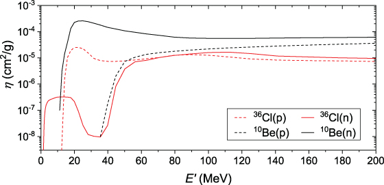
Figure 4.2. Function
 (see Equation (4.2)) for the
production of 10Be (black curves) and 36Cl (red) in air by
protons (dotted curves) and neutrons (solid) with energy
(see Equation (4.2)) for the
production of 10Be (black curves) and 36Cl (red) in air by
protons (dotted curves) and neutrons (solid) with energy
 . The cross sections of the
corresponding reactions were taken from Webber & Higbie (2003) and Beer et al. (2012).
. The cross sections of the
corresponding reactions were taken from Webber & Higbie (2003) and Beer et al. (2012).
Download figure:
Standard image High-resolution imageIn earlier years,
 was typically calculated using analytical
approximations or semiempirical approaches to model the nucleonic cascade in the
atmosphere (see, e.g., Lal & Peters 1962; Lingenfelter 1963; O'Brien 1979). With the fast growth of
computational power in recent decades, a more precise and physical Monte Carlo
approach was developed to compute the cascade details. This method requires massive
computations (it may take up to 108 simulated incident particles per one
energy point), but offers high precision and full physical understanding including all
known effects. For that purpose, many sophisticated codes have been developed, which
can be used to simulate the cosmic-ray-induced atmospheric cascade. The most widely
used codes are CORSIKA (COsmic Ray SImulations for KAscade), which was designed
specifically for the simulation of air showers from high-energy galactic cosmic rays
(Heck et al. 1998);
MCNP (Monte Carlo N-Particle Transport) with an emphasis on accurate simulation of
neutron transport (Werner et al. 2017); general-purpose FLUKA (Ferrari et
al. 2005; Böhlen et al.
2014) and GEANT4
(GEometry ANd Tracking, v. 4; Agostinelli et al. 2003; Allison et al. 2006); and some others.
was typically calculated using analytical
approximations or semiempirical approaches to model the nucleonic cascade in the
atmosphere (see, e.g., Lal & Peters 1962; Lingenfelter 1963; O'Brien 1979). With the fast growth of
computational power in recent decades, a more precise and physical Monte Carlo
approach was developed to compute the cascade details. This method requires massive
computations (it may take up to 108 simulated incident particles per one
energy point), but offers high precision and full physical understanding including all
known effects. For that purpose, many sophisticated codes have been developed, which
can be used to simulate the cosmic-ray-induced atmospheric cascade. The most widely
used codes are CORSIKA (COsmic Ray SImulations for KAscade), which was designed
specifically for the simulation of air showers from high-energy galactic cosmic rays
(Heck et al. 1998);
MCNP (Monte Carlo N-Particle Transport) with an emphasis on accurate simulation of
neutron transport (Werner et al. 2017); general-purpose FLUKA (Ferrari et
al. 2005; Böhlen et al.
2014) and GEANT4
(GEometry ANd Tracking, v. 4; Agostinelli et al. 2003; Allison et al. 2006); and some others.
During the last decades, several Monte Carlo models have been developed to compute the production of different cosmogenic isotopes. Masarik & Beer (1999, 2009) based their model on the GEANT+MCNP code; Webber & Higbie (2003) and Webber et al. (2007) used FLUKA; Usoskin & Kovaltsov (2008), Kovaltsov & Usoskin (2010), and Leppänen et al. (2012) used the CORSIKA and FLUKA codes; Kovaltsov et al. (2012) used the PLANETOCOSMICS tool (Desorgher et al. 2005) based on GEANT4; and Matthiä et al. (2013), Pavlov et al. (2017), and Poluianov et al. (2016) used GEANT4. The results of the different simulations may be slightly different because of different physical models of particle interactions (e.g., Kang et al. 2013; Pavlov et al. 2017). Here we show, as illustration, the results for the model (Poluianov et al. 2016), unless stated otherwise.
Beryllium isotopes are produced in the atmosphere as a result of the spallation of nitrogen and oxygen, with the energy threshold of several tens of megaelectronvolts. The lowest value of the threshold (12 MeV) is for the reaction 14N(n,αp)10Be, which has the maximum at the neutron energy around 20–30 MeV (see Figure 4.2).
Chlorine-36 is produced mostly as a product of spallation of the most abundant argon
isotope 40Ar, which is 99.6% of all atmospheric argon. The reaction
40Ar(p,αn)36Cl has a lower threshold
( 9 MeV) and a maximum at 20–30 MeV. However,
the much less abundant isotope 36Ar can also significantly contribute to
the production of 36Cl because of the reaction
36Ar(n,p)36Cl, which has no threshold and a high cross section
at low energies. Because of the low abundance of argon versus oxygen and nitrogen in
the atmosphere, the production rate of 36Cl is roughly an order of
magnitude lower than that of 10Be.
9 MeV) and a maximum at 20–30 MeV. However,
the much less abundant isotope 36Ar can also significantly contribute to
the production of 36Cl because of the reaction
36Ar(n,p)36Cl, which has no threshold and a high cross section
at low energies. Because of the low abundance of argon versus oxygen and nitrogen in
the atmosphere, the production rate of 36Cl is roughly an order of
magnitude lower than that of 10Be.
Radiocarbon 14C is produced in another type of reaction. By far the most
important channel of 14C production is the exothermic reaction
14N(n,p)14C, sometimes called neutron capture. The other
channel, spallation reaction 16O(p,3p)14C, has a high energy
threshold and low cross section; thus, its contribution to the total atmospheric
production is negligible. The cross section of the main reaction inversely depends on
the energy of neutrons,
 (
( ), so that the lower the neutron's energy
is, the more effectively it is captured by nitrogen. Because of that, energetic
neutrons get thermalized in elastic scattering with nuclei of atmospheric gases before
being captured. This process leads to the diffusion of neutrons in the atmosphere
which should be taken into account in computations of the altitudinal profile of
14C production in the atmosphere. Because this process is relatively
fast, the decay of neutrons and their leakage from the atmosphere can be typically
ignored.
), so that the lower the neutron's energy
is, the more effectively it is captured by nitrogen. Because of that, energetic
neutrons get thermalized in elastic scattering with nuclei of atmospheric gases before
being captured. This process leads to the diffusion of neutrons in the atmosphere
which should be taken into account in computations of the altitudinal profile of
14C production in the atmosphere. Because this process is relatively
fast, the decay of neutrons and their leakage from the atmosphere can be typically
ignored.
4.2.2. Production Function
In earlier years, it was usual to compute the cosmogenic isotopes production using Equation (4.1) directly for a prescribed spectrum of primary cosmic rays (e.g., Masarik & Beer 1999). However, this ties the result to the fixed spectral shape and does not make it possible to model the isotope production for other spectral shapes, for example, for SEPs. For computations of the isotope production in the atmosphere, it is much more practical to use the so-called production function S(E, d) (in units of atoms g−1 cm2), which gives the production of the cosmogenic isotope (number of atoms) at a given atmospheric level d per primary particle impinging on the top of the atmosphere with initial energy E (e.g., Webber et al. 2007; Poluianov et al. 2016). The production function is typically computed for the isotropic angular distribution of the primary particles on the top of the atmosphere, which is a valid assumption for GCR and less so for SEP sources. The full model of the function S for the production of 10Be, 14C, 36Cl, and other cosmogenic isotopes by primary protons and α-particles (the latter effectively includes heavier species) was presented by Poluianov et al. (2016; see also the supporting information therein).
Examples of the altitude profile of the production function
S(E, d) are shown in Figure 4.3. One can see that for
low-energy incident particles (panel A), the profile of 10Be and
36Cl is mostly defined by direct reactions of the primaries in the upper
layers (small d) in the atmosphere, while the secondaries are less
effective, which is observed as a second "step" in the distribution at depths
 . For higher energy primary particles (panel
B), the atmospheric cascade (Figure 2.12) is fully developed, defining the
profile of the production, which has a maximum at the depth of a few tens of g
cm−2 with an exponential decay to deeper layers. Although proton cross
sections are greater than neutron ones (see the 36Cl curves in Figure 4.2), production is mostly
defined by secondary neutrons, as protons are quickly stopped in the atmosphere by
Coulomb losses, having a smaller chance to initiate a reaction. Altitude profiles of
14C production are totally defined by the secondary neutron production
and thermalization, and has a typical pattern with a maximum at ∼100 g cm−2
depth (the so-called Pfotzer–Regener maximum of the greatest intensity of secondary
nucleons of the atmospheric cascade).
. For higher energy primary particles (panel
B), the atmospheric cascade (Figure 2.12) is fully developed, defining the
profile of the production, which has a maximum at the depth of a few tens of g
cm−2 with an exponential decay to deeper layers. Although proton cross
sections are greater than neutron ones (see the 36Cl curves in Figure 4.2), production is mostly
defined by secondary neutrons, as protons are quickly stopped in the atmosphere by
Coulomb losses, having a smaller chance to initiate a reaction. Altitude profiles of
14C production are totally defined by the secondary neutron production
and thermalization, and has a typical pattern with a maximum at ∼100 g cm−2
depth (the so-called Pfotzer–Regener maximum of the greatest intensity of secondary
nucleons of the atmospheric cascade).
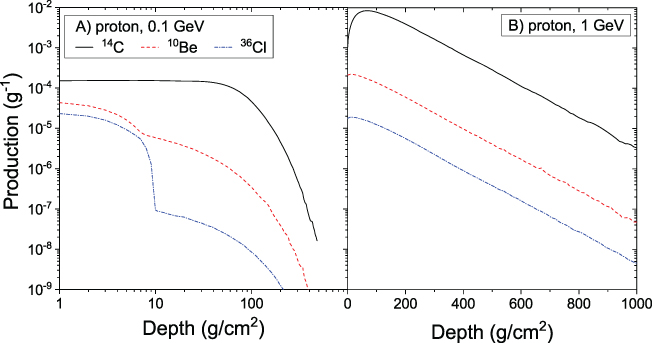
Figure 4.3. Altitude profile of the production function S(E, d) for isotopes 10Be, 14C, and 36Cl by primary protons with energies 0.1 GeV (panel A) and 1 GeV (panel B), for the computations by Poluianov et al. (2016). Note the logarithmic and linear scales for the depth axes in panels A and B, respectively.
Download figure:
Standard image High-resolution imageBy integrating the production function over depth, one can obtain the columnar production (viz. integrated within the entire atmospheric column) of the cosmogenic isotope (e.g., Webber et al. 2007; Kovaltsov et al. 2012):

where D = 1033 g cm−2 is the atmospheric depth at the mean sea level. The columnar production gives the total number of isotope atoms per primary particle in the entire atmosphere. Columnar productions of the isotopes 10Be, 14C and 36Cl for primary protons are shown in Figure 4.4 (panel A) in comparison with the yield function (see below) of a standard sea-level neutron monitor.
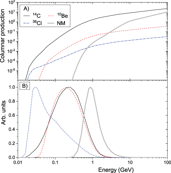
Figure 4.4. (A) Columnar production SC(E) (in atoms cm2 g−1) for 10Be, 14C, and 36Cl as a function of the energy of primary protons (Poluianov et al. 2016). NM denotes the yield function of a standard sea-level neutron monitor (Mishev et al. 2013, in arbitrary units). (B) Differential response functions of cosmogenic isotopes for the hard-spectrum SEP event on 1956 February 23. The response of a polar sea-level neutron monitor (NM in the legend) is shown for comparison. The functions are normalized to their maxima.
Download figure:
Standard image High-resolution imageThe production function is computed for one incident primary particle, but cosmic
rays are usually quantified via the intensity in units of particles (cm2 s
sr)−1. Therefore, instead of the production function S,
the yield function Y is used, which is defined as the production (the
number of atoms per gram of air) of the isotope, at the given atmospheric depth
d by primary particles of type i with units of
intensity. The units of Y are (atoms g−1 cm2
sr). For the isotropic angular distribution of primary cosmic rays near Earth, the
yield function is related to the production function as
 .
.
The production rate Q of cosmogenic isotope can be defined as an
integral of the product of the yield function and the differential energy spectrum of
cosmic rays  (in particles (cm2 s
sr)−1) above the energy Ec corresponding to
the local geomagnetic cutoff rigidity Pc:
(in particles (cm2 s
sr)−1) above the energy Ec corresponding to
the local geomagnetic cutoff rigidity Pc:

where the summation is
over different types of primary cosmic-ray particles (protons,
α-particles, etc.). The relation between
 and the local geomagnetic rigidity cutoff
Pc (defined independently) is
and the local geomagnetic rigidity cutoff
Pc (defined independently) is

where Zi and Ai are the charge and mass numbers of particles of type i, respectively; Er = 0.938 GeV is the rest mass of a proton.
While all types of primary cosmic-ray particles (protons and heavier nuclei) should
be considered for GCR, because
 particles can contribute up to half of the
production, only protons are usually taken for SEP events.
particles can contribute up to half of the
production, only protons are usually taken for SEP events.
The global production rate QG of an isotope can be computed as the spatial average over the global columnar production rate, defined as

where Q is given by Equation (4.4), and integration is over the entire atmospheric column (as in the columnar production) and over Earth's surface (longitude and latitude) Ω.
Cosmogenic Isotope Production by SEPs
Figure 4.5 (panel A) depicts the distribution of the global production rate of 10Be over different latitudinal bands for a hard-spectrum SEP event and for moderately modulated GCR. Panel B of the same figure depicts the fraction of tropospheric production in 10° latitudinal bands to the total production in the same bands. One can see that 10Be is mostly produced by SEP at high latitudes (60°–80°), and the tropospheric production is small. On the other hand, GCR produce the isotope more evenly over the latitude, and a significant fraction is produced in the troposphere. This pattern is also typical for other isotopes.
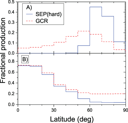
Figure 4.5. (A) Fraction of the columnar 10Be production in latitudinal bands (10° wide) to the global production for two scenarios: a hard-spectrum SEP event (1956 February 23) and moderately modulated (ϕ = 600 MV) GCR. (B) Fraction of the tropospheric production of 10Be to the total columnar production in different latitudinal bands, for the same scenarios. Computations were done according to the model (Poluianov et al. 2016).
Download figure:
Standard image High-resolution imageTable 4.2 collects the quantities of the global isotope production in the atmosphere for the event of 775 CE assuming hard (similar to that of the GLE on 1956 February 23) and soft (similar to that of the GLE on 1972 August 4) SEP spectra.
Figure 4.4(B) depicts the so-called "differential response function" for the cosmogenic isotope production, which is a product of the production function SC(E) and the hard SEP energy spectrum Jp(E). Because isotope production by SEPs takes place mostly at high latitudes with no or low geomagnetic rigidity cutoff, this differential response function allows one to evaluate the most effective energy ranges for the production of different isotopes. One can see from the figure that 10Be and 14C have very close effective energy ranges for SEP events (a few hundred megaelectronvolts to about 1 GeV) owing to their similarly shaped columnar production functions (panel A). In contrast, 36Cl is most effectively produced by SEPs with a significantly lower energy of tens of megaelectronvolts, owing to the low-energy production channel with the reaction 36Ar(n,p)36Cl. This feature makes it possible to estimate, using simultaneous measurements of different isotopes produced by an extreme SEP event, the SEP spectrum in the energy range between tens and hundreds of megaelectronvolts (see Section 6.2).
Table 4.2. Cosmogenic Isotope Production (Following the Model of Poluianov et al. 2016) by an Extreme SEP Event (Corresponding to the Event of 775 CE for Hard and Soft Energy Spectra) and GCR (Solar Minimum and Maximum Conditions)
| SEP Event | GCR | |||
|---|---|---|---|---|
| Hard | Soft | ϕ = 400 MV | ϕ = 1000 MV | |
| Globally averaged production | ||||
| 14C† |

|

|

|

|
| Tropospheric fraction in the total global production | ||||
| Rtrop(14C) | 0.073 | 0.007 | 0.32 | 0.36 |
| Rtrop(10Be) | 0.049 | 0.003 | 0.30 | 0.34 |
| Rtrop(36Cl) | 0.033 | 0.0003 | 0.30 | 0.35 |
| Total atmospheric production ratios | ||||
| 14C/10Be | 46 | 45 | 55 | 56 |
| 14C/36Cl | 340 | 62 | 631 | 645 |
Notes. The parameters are the globally averaged production (in cm−2) of 14C for the 775 CE event (Güttler et al. 2015) (left block) and the annual production by GCR (right block), the tropospheric fraction Rtrop (with a realistic tropopause profile) in the total global production for the three isotopes, and the ratio of the total atmospheric production of two isotope pairs.
In Figure 4.6, we show the ratio of the modeled production of different cosmogenic isotopes as a function of the softness (quantified via the ratio of the integral fluences F30/F200—see Section 2.2 for definitions) of the SEP spectrum for all GLE events recorded after 1956 (Raukunen et al. 2018). One can see that the ratio for 14C/10Be is nearly independent of the spectral softness, varying within less than a factor of 2 over two orders of its magnitude. Accordingly, the ratio of these two isotopes does not provide direct information on the particle spectrum. On the other hand, the ratio of 36Cl/10Be is tightly linked to the softness index, varying by nearly an order of magnitude between soft- and hard-spectrum events. This allows the SEP spectrum to be estimated directly from the measured isotope ratio (see Section 6.2).
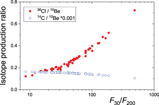
Figure 4.6. Ratio of modeled productions of cosmogenic isotopes (as denoted in the legend) as a function of the integral fluences F30/F200 (Section 2.2) for the observed GLE events of 1956–2012 (Raukunen et al. 2018). For 14C, global production is considered, while for 10Be and 36Cl, it is the polar deposition calculated using the atmospheric transport/deposition according to Heikkilä et al. (2009).
Download figure:
Standard image High-resolution imageCosmogenic isotopes in natural archives are often called "a natural neutron
monitor" (e.g., Beer 2000). This is correct in the sense that cosmogenic isotopes are also an
integral detector, with the columnar production of cosmogenic isotopes similar to
the yield function of a polar neutron monitor (Figure 4.4(A)). However, they are not identical,
because the effective energy ranges of the isotopes and NMs are different (see
Figure 4.4(B)),
particularly for SEP events. Cosmogenic isotopes, especially 36Cl, are
more sensitive to lower energies than a standard sea-level NM is. While the
effective energy for SEP/GLE Eeff is
 for 14C and 10Be
(Kovaltsov et al. 2012), it is much higher for a sea-level polar NM, being
for 14C and 10Be
(Kovaltsov et al. 2012), it is much higher for a sea-level polar NM, being
 (Koldobskiy et al. 2018).
4.2.3. Production of Cosmogenic Isotopes by γ-radiation
It is not only energetic ions of GCR and SEP but also γ-radiation from nearby supernovae (SN) or gamma-ray bursts (GRBs) that can potentially lead to the production of cosmogenic isotopes (Menjo et al. 2005; Hambaryan & Neuhäuser 2013). Details of the cosmogenic production of long-living isotopes by primary γ-radiation are provided by, e.g., Pavlov et al. (2013a, 2013b).
Figure 4.7 shows the production functions for 14C, 10Be, and 36Cl in Earth's atmosphere by primary γ-radiation, according to a recent model (Pavlov et al. 2013a). Photonuclear reactions of photons with energy above 10 MeV lead to generation of secondary neutrons and protons, which further produce cosmogenic isotopes in a way similar to that descried above for incident ions. The maximum of the γ-ray production function for 14C corresponds to the giant dipole resonance of photonuclear reactions on the target nuclei of nitrogen and oxygen. In this energy range, photons produce secondary neutrons and protons with energy of several megaelectronvolts, which is below the spallation threshold of 10Be production on nitrogen and oxygen. Production of 10Be becomes significant when the photon's energy reaches 50 MeV or more and goes in both direct photodisintegration reactions and spallation reactions by secondary nucleons. Because typical spectra of γ-quanta for SN and RGB sources are steep, this leads to a much smaller production ratio 10Be/14C than the one for GCR or SEP. Detailed simulations (Pavlov et al. 2013b, 2014) yield the expected ratio of 14C/10Be of 400–800 versus ∼50 for energetic particles (see Table 4.2). Production of 36Cl on 40Ar by photons is similarly suppressed, leading to an even greater ratio of 14C/36Cl of 800–1600 (Pavlov et al. 2013b, 2014). As in the case of SEPs, the production of cosmogenic isotopes by γ-quanta takes place dominantly in the stratosphere. On the other hand, because photons are not deflected by the geomagnetic field, the production is limited not to the polar regions but to the spot on Earth irradiated by photons.
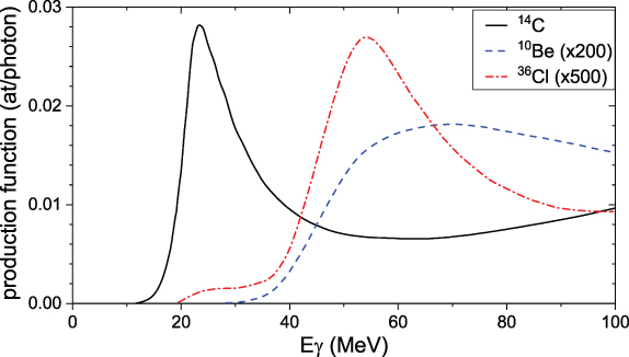
Figure 4.7. Cosmogenic isotope production functions by primary γ-quanta in Earth's atmosphere, using yield functions from Pavlov et al. (2013a). For better visibility, curves for 10Be and 36Cl are scaled up by factors of 200 and 500, respectively.
Download figure:
Standard image High-resolution imageThus, the ratio of nuclides produced in the atmosphere may clearly distinguish cases related to energetic particles and γ-radiation. In the latter case, no measurable signal by γ-radiation is expected in 10Be or 36Cl even for such a pronounced 14C spike as for the 775 CE event. Both beryllium and chlorine spikes were measured for the events discussed here. This fact ultimately rejects the proposed earlier hypothesis (Hambaryan & Neuhäuser 2013; Miyake et al. 2012; Pavlov et al. 2013a) that they were caused by SN/GRBs.
4.3. Isotope Transport
Eugene Rozanov, Aryeh Feinberg, and Timofei Sukhodolov
All isotopes considered here are produced mostly by galactic cosmic rays in the lower extratropical stratosphere and are transported by atmospheric air motions to natural archives such as ice sheets and tree rings, where they can be detected and measured.
4.3.1. Atmospheric Air Advection Pathways
Atmospheric circulation is air motion driven by many forces acting in the rotating atmosphere of Earth. The most important driving forces are the inhomogeneity of the solar radiative heating, Coriolis force, and forcing from atmospheric waves (e.g., Holton 2004). The joint action of these forces is responsible for large-scale circulation features, which are relatively persistent on long-term timescales. The zonal mean structure of the main atmospheric advective transport pathways is shown in Figure 4.8.
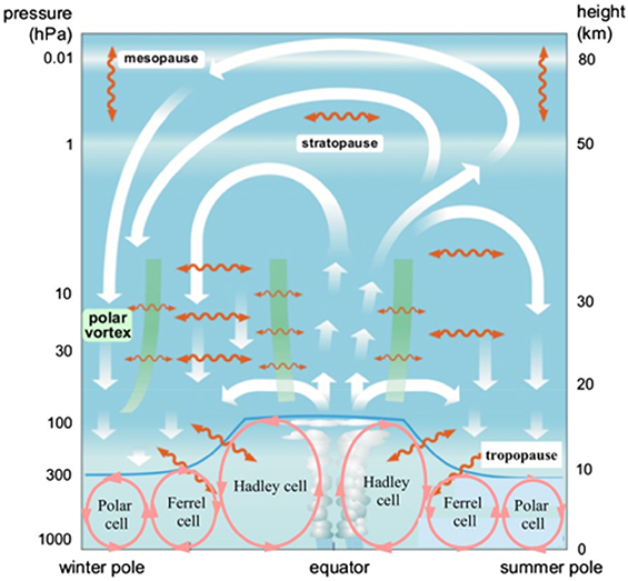
Figure 4.8. The atmospheric circulation cells. Adapted from Boenisch et al. (2011) and Proedrou & Hocke (2016) CC BY 3.0. White arrows illustrate the two stratospheric circulation branches. Tropospheric circulation cells are shown with red circles. Macroturbulent mixing is shown by the wavy orange lines. Green bands illustrate the transport barriers.
Download figure:
Standard image High-resolution imageIn the stratosphere, advective mass transfer, known as the Brewer–Dobson circulation
(BDC hereafter), is carried out by two circulation cells. They both start from the
tropical upwelling driven mostly by tropospheric convection. The poleward and
descending motions are driven by the forcing from the breaking of vertically
propagating planetary, synoptic-scale, and gravity waves (Plumb 2002). The seasonal behavior of the BDC
branches is driven by solar radiative heating directly in the stratosphere as well as
indirectly from the changing wave forcing, due to solar irradiance absorption lower in
the troposphere. Seasonality is expressed as atmospheric polar night (geographical
latitude  ) and extratropical jet variability. Polar
night jets appear on the edges of the polar night area and therefore the upper BDC
branch provides more intensive downward transport in the winter hemisphere. The
seasonal behavior of the extratropical jets is not very pronounced, leading to a weak
seasonal cycle of shallow BDC branch intensity. Advective transport is constrained by
transport barriers, where the absence of wave forcing does not provide the necessary
conditions for the poleward/downward advective mass transport. In the troposphere, the
zonal mean mass transport follows three circulation cells (Polar, Ferrel, and Hadley)
covering the entire troposphere. These cells provide rather fast (up to six months
between equator and high latitudes) hemispheric transport of the material that entered
the troposphere. The interhemispheric transport timescale in the troposphere is
longer, reaching a timescale of around one to two years.
) and extratropical jet variability. Polar
night jets appear on the edges of the polar night area and therefore the upper BDC
branch provides more intensive downward transport in the winter hemisphere. The
seasonal behavior of the extratropical jets is not very pronounced, leading to a weak
seasonal cycle of shallow BDC branch intensity. Advective transport is constrained by
transport barriers, where the absence of wave forcing does not provide the necessary
conditions for the poleward/downward advective mass transport. In the troposphere, the
zonal mean mass transport follows three circulation cells (Polar, Ferrel, and Hadley)
covering the entire troposphere. These cells provide rather fast (up to six months
between equator and high latitudes) hemispheric transport of the material that entered
the troposphere. The interhemispheric transport timescale in the troposphere is
longer, reaching a timescale of around one to two years.
4.3.2. Atmospheric Diffusion/Mixing
The isotopes are also involved in different diffusion processes driven by turbulent mixing caused by air flow fluctuations and the formation of different vortices or eddies. These vortices can absorb the air parcel and move it for some distance until destruction and final mixing with ambient air. This process is called turbulent or eddy diffusion and usually works in the direction perpendicular to the air flow or in the case when strong horizontal/vertical gradients of the gas or aerosol mixing ratios appears. In the stratosphere, eddy transport is driven by breaking waves, which form eddies (Plumb 2002). The turbulent mixing pathways are shown by the wavy orange lines in Figure 4.8. This mechanism is especially important for the transport of species across their production area boundaries. For example, enhanced vertical ozone diffusion across the tropopause occurs in the summer season, when the ozone mixing ratio in the stratosphere exceeds its tropospheric values (e.g., Škerlak et al. 2014). The intensity of the eddy transport also depends on atmospheric properties and substantially varies in space and time. Irregularities of the air flows in the planetary boundary layer produce very intensive turbulent mixing during the day time, while in more quiet night-time conditions, the mixing intensity is greatly reduced. The representation of mixing processes in the numerical isotope transport models depends on the model complexity. In a simplified box, 1D and 2D models of the description of mixing are based on the application of empirical turbulent diffusion coefficients acquired from observation analysis (e.g., Talpos & Cuculeanu 1997). In the case of general circulation models, some part of the eddy transport related to the resolved waves is treated by the dynamical core and transport module, while the other mixing processes need to be parameterized (Heikkilä et al. 2013). The isotopes can also be transported by small-scale convection in the troposphere. Convective motions are generated in unstable tropospheric layers, when the vertical temperature gradient is larger than either the dry or the wet adiabatic lapse rates. In this case, the air parcel being moved up tends to remain in this direction because it stays warmer than ambient air. In the dry convection case, the air is distributed fast and uniformly in the air column (e.g., Jacob & Prather 1990). This process is active mostly during the day time in the planetary boundary layer from the surface to approximately 1–2 km altitude. The treatment of this process in models is based on the analysis of the temperature gradient to define regions with unstable stratification. Moist convection can generate vertically extended or convective clouds and substantially contributes to the intensity of vertical mixing in the troposphere, accelerating surface-to-tropopause exchange from weeks to hours (e.g., Tost et al. 2010). Overall, convective mixing is less important for cosmogenic isotopes because they are produced mostly in the stratosphere; however, it can accelerate their downward propagation after they cross the tropopause.
4.3.3. Transport from the Stratosphere to the Lower Troposphere
The most important component of isotope transport is the transport across the tropopause, i.e., from the stratosphere to the lower troposphere, which is also known as the stratosphere–troposphere transport (STT). The main mechanisms are related to advective downward air motion as part of the BDC, mixing across the tropopause and the presence of stratospheric air intrusions through tropopause discontinuities. Figure 4.9 illustrates the main pathways of stratospheric air propagation to the lower troposphere: quasi-horizontal eddy transport through the middle-latitude tropopause (wavy orange arrows) and advective downward propagation across the polar tropopause as part of the large-scale BDC (blue arrows). According to Liang et al. (2009), the stratospheric air penetrating through the tropopause can reach the surface in approximately three months. This transport time agrees reasonably well with the results from Stohl (2006), who estimated that the mean time of the air transport from the tropopause to the lower troposphere is about 100 days; however, it was also mentioned that the transport to the Arctic and tropical lower troposphere could take longer. During this process, stratospheric air is also involved in intensive mixing between the middle and high latitudes caused by large-scale advection (see Figure 4.8), as well as by mixing via tropospheric eddies and vortices (cyclones and anticyclones), which lead to approximately one month for the mixing of the middle latitudes and the polar air masses. It was also found out (Liang et al. 2009) that 67%–81% of the stratospheric air in the NH troposphere arrived via stratosphere–troposphere transport (STT) over the midlatitudes.

Figure 4.9. A schematic diagram of stratospheric air transport to the lower troposphere (Holton et al. 1995; Liang et al. 2009; CC BY 3.0.). Quasi-horizontal eddy transport over middle latitudes is shown by the wavy arrows. Slow advective downward transport through the polar tropopause is marked by blue arrows. The transport inside the troposphere is shown by orange and blue arrows. The values in percent illustrate the stratospheric contribution from STT over the middle (red) and high (blue) latitudes.
Download figure:
Standard image High-resolution image4.3.4. Carbon Cycle
Radiocarbon 14C produced by cosmic rays becomes gaseous CO2 through CO. After the atmospheric transport described above, 14C concentrations in the troposphere become nearly uniform. Trees, the main archive sample of 14C, absorb CO2 by photosynthesis. Therefore, the 14C concentrations of tree rings reflect tropospheric conditions.
Carbon transport occurs not only in the atmosphere but also in various types of reservoirs such as oceans and biotas, and such transport is known as the global carbon cycle. Reservoirs define spaces on the globe for the movement and storage of matter. Each reservoir can be considered uniform to a certain extent with respect to general properties, such as composition, pressure, and temperature, and is separated by discontinuous surfaces. Reservoirs are mainly divided into the atmosphere, oceans, and biosphere. The carbon exchange between the atmosphere and seawater is caused by changes in CO2gas and CO2aq, and that between the atmosphere and biosphere is caused by photosynthesis and the respiration of plants and decomposition of organic matter by microbes. These aforementioned reservoirs of the atmosphere, oceans, and biosphere can also be classified according to their characteristics: e.g., the atmosphere is often divided into two subreservoirs—the stratosphere and troposphere. The state in which the inflow and outflow of matter in each reservoir are balanced is called the steady state. In this state, carbon fluxes of the inflow and outflow in each reservoir, often expressed as GtC (gigaton carbon) per year, are equal, i.e., a reservoir size (total carbon amount of each reservoir) is constant. Such a concept of carbon transfer between reservoirs is known as a box model. The sizes of reservoirs and carbon fluxes between reservoirs are determined using present-day observations or at the bomb peak (see Section 7.1). Figure 4.10 shows a recent box model by Büntgen et al. (2018). This box model details the main reservoirs, reservoir sizes, and fluxes between them.

Figure 4.10. 22 box carbon-cycle model for the preindustrial era. Each hemisphere has 11 reservoirs (boxes). The number in each box indicates the total carbon mass (GtC). The arrows indicate the carbon fluxes between boxes (GtC/year). Reproduced from Büntgen et al. (2018), CC BY 4.0.
Download figure:
Standard image High-resolution imageTree-ring 14C data (in particular, with a resolution worse than one year) show nearly uniform tropospheric values, so that the 14C difference between tree-ring regions is small. Therefore, previous researches have estimated that cosmic-ray-induced 14C production rates via 14C concentrations of tree rings mainly using this type of box model. Calculations made using such a box model often only required the 14C production rate input into the atmospheric reservoir (used as a variable parameter). However, regional differences in 14C concentrations exist. The most remarkable regional difference is known as an interhemispheric offset, i.e., 14C concentrations in the southern hemisphere show lower values than those in the northern hemisphere (Hogg et al. 2013). This is explained by the higher fraction of oceanic area comprising the southern hemisphere (because 14C is mainly produced in the atmosphere, the atmospheric reservoir has a higher 14C concentration than the marine reservoir). As described above, because the stratosphere–troposphere exchange occurs at mid to high latitudes, it is considered that the 14C concentration at these latitudes is higher than at the equator (Hua & Barbetti 2014).
Recent 14C measurements with improved temporal and spatial resolution have emphasized such regional 14C differences and seasonal 14C variations (Büntgen et al. 2018; Uusitalo et al. 2018). Although the differences between the northern and southern hemispheres were explained in the detailed box model (Figure 4.10), it is quite difficult to explain 14C data which possess higher spatial resolution by using box models. In addition, changes in the carbon cycle caused by climate change cannot be dealt with by the box model, which assumes steady state. Recently, 14C production rates were reconstructed using Bern3D-LPJ (Figure 4.11), which is a dynamic model of a realistic three-dimensional time-dependent transport and distribution of radiocarbon (Roth & Joos 2013). In the future, an interpretation using such 3D carbon-cycle models will be important, particularly with the available high-precision (both spatial and temporal resolution) 14C data.

Figure 4.11. Schematic presentation of the Bern3D-LPJ carbon-cycle–climate model. Gray arrows
denote externally applied forcings resulting from variations in greenhouse gas
concentrations and aerosol loading, orbital parameters, ice-sheet extent, and
sea-level and atmospheric CO2 and
 14C. The atmospheric energy
and moisture balance model (blue box and arrows) communicate interactively the
calculated temperature, precipitation, and irradiance to the carbon-cycle model
(light brown box). The production and exchange fluxes of radiocarbon (red) and
carbon (green) within the carbon-cycle model are sketched by arrows, where the
width of the arrows indicates the magnitude of the corresponding fluxes in a
preindustrial steady state. The two maps show the depth-integrated inventories of
the preindustrial 14C content in the ocean and land modules in units of
103 mol 14C
m−2/14
Rstd. Reproduced from
Roth & Joos (2013), CC BY 3.0.
14C. The atmospheric energy
and moisture balance model (blue box and arrows) communicate interactively the
calculated temperature, precipitation, and irradiance to the carbon-cycle model
(light brown box). The production and exchange fluxes of radiocarbon (red) and
carbon (green) within the carbon-cycle model are sketched by arrows, where the
width of the arrows indicates the magnitude of the corresponding fluxes in a
preindustrial steady state. The two maps show the depth-integrated inventories of
the preindustrial 14C content in the ocean and land modules in units of
103 mol 14C
m−2/14
Rstd. Reproduced from
Roth & Joos (2013), CC BY 3.0.
Download figure:
Standard image High-resolution image4.3.5. Gravitational Sedimentation
Some of the isotopes (e.g., 14C) form gases, and their transport in the atmosphere depends on the above-mentioned processes. Other isotopes form ion clusters or primary particles, which can be captured by different aerosols (Junge 1963; Lal & Peters 1967). In this case, the transport can be enhanced or suppressed by gravitational sedimentation. Figure 4.12 shows the gravitational settling speed for the spherical sulfate aerosol particles in the lower stratosphere (Pierce et al. 2010).
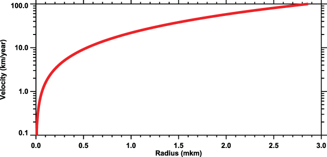
Figure 4.12. Gravitational settling velocity of sulfate aerosols at 25 km altitude as a function of their size as based on the relation from Seinfeld & Pandis (2006).
Download figure:
Standard image High-resolution imageThe sulfate aerosol particle radius is usually less than
 (Figure 2 in Pierce et al. 2010), with a modal value
at
(Figure 2 in Pierce et al. 2010), with a modal value
at  . For these particles, the gravitational
sedimentation velocity ranges between 200 m yr−1 and 1 km yr−1
and does not play an important role in the lower stratosphere, where it is much
smaller than the vertical wind speed (e.g., Weisenstein et al. 2015; Zhou et al. 2006). After a strong volcanic eruption,
the size distribution is shifted to larger values. Stratospheric aerosol particles
after Pinatubo had mean radii around 0.6 and
. For these particles, the gravitational
sedimentation velocity ranges between 200 m yr−1 and 1 km yr−1
and does not play an important role in the lower stratosphere, where it is much
smaller than the vertical wind speed (e.g., Weisenstein et al. 2015; Zhou et al. 2006). After a strong volcanic eruption,
the size distribution is shifted to larger values. Stratospheric aerosol particles
after Pinatubo had mean radii around 0.6 and
 (Figure 3 in Pierce et al. 2010) in the tropical and
lower middle-latitude stratosphere, respectively, which sediment at around 10 and 6 km
yr−1. These values are comparable to advective upward motions speed in
the tropical BDC branch (Weisenstein et al. 2015), preventing aerosol (with embedded
isotopes) from being transported to the middle stratosphere. Over the middle
latitudes, the annual mean downward wind speed is around 10 km yr−1 (e.g.,
Zhou et al. 2006), but
can reach higher values during the dynamically active winter season. In this case, the
downward advective transport of the volcanic aerosol across the tropopause can be
substantially enhanced by sedimentation. Some evidences of this enhancement have been
identified (Baroni et al. 2011, 2019),
in the form of a simultaneous increase in cosmogenic 10Be and sulfate
deposition in polar ice cores after powerful stratospheric volcanic eruptions. This
fact contradicts earlier statements (e.g., Lal & Peters 1967) about the marginal importance of
gravitational settling and identical transport of isotopes in gas and aerosol forms.
Gravitational sedimentation can also be important in the middle/upper stratosphere
even for background aerosol because of gravitational sedimentation speed increasing
with altitude. It was estimated (Figure 1(a) in Weisenstein et al. 2015) that in the tropical
stratosphere, the sedimentation speed of an aerosol particle with
(Figure 3 in Pierce et al. 2010) in the tropical and
lower middle-latitude stratosphere, respectively, which sediment at around 10 and 6 km
yr−1. These values are comparable to advective upward motions speed in
the tropical BDC branch (Weisenstein et al. 2015), preventing aerosol (with embedded
isotopes) from being transported to the middle stratosphere. Over the middle
latitudes, the annual mean downward wind speed is around 10 km yr−1 (e.g.,
Zhou et al. 2006), but
can reach higher values during the dynamically active winter season. In this case, the
downward advective transport of the volcanic aerosol across the tropopause can be
substantially enhanced by sedimentation. Some evidences of this enhancement have been
identified (Baroni et al. 2011, 2019),
in the form of a simultaneous increase in cosmogenic 10Be and sulfate
deposition in polar ice cores after powerful stratospheric volcanic eruptions. This
fact contradicts earlier statements (e.g., Lal & Peters 1967) about the marginal importance of
gravitational settling and identical transport of isotopes in gas and aerosol forms.
Gravitational sedimentation can also be important in the middle/upper stratosphere
even for background aerosol because of gravitational sedimentation speed increasing
with altitude. It was estimated (Figure 1(a) in Weisenstein et al. 2015) that in the tropical
stratosphere, the sedimentation speed of an aerosol particle with
 radius increases from 1 km yr−1
at 20 km to almost 100 km yr−1 at 50 km. The role of gravitational
sedimentation was evaluated by Delaygue et al. (2015) using numerical experiments with a 2D
model, which includes detailed sulfate aerosol microphysics. An experiment with
gravitational sedimentation switched off was compared with a reference model run with
all processes switched on. The ratio of 10Be concentrations simulated
without and with sedimentation of particles is presented in Figure 4.13. The main effects are
confined to the middle/upper stratosphere, where 10Be accumulates when
gravitational sedimentation is turned off. It is interesting to note that
gravitational sedimentation does not contribute to the 10Be distribution
around the tropopause in nonvolcanic conditions.
radius increases from 1 km yr−1
at 20 km to almost 100 km yr−1 at 50 km. The role of gravitational
sedimentation was evaluated by Delaygue et al. (2015) using numerical experiments with a 2D
model, which includes detailed sulfate aerosol microphysics. An experiment with
gravitational sedimentation switched off was compared with a reference model run with
all processes switched on. The ratio of 10Be concentrations simulated
without and with sedimentation of particles is presented in Figure 4.13. The main effects are
confined to the middle/upper stratosphere, where 10Be accumulates when
gravitational sedimentation is turned off. It is interesting to note that
gravitational sedimentation does not contribute to the 10Be distribution
around the tropopause in nonvolcanic conditions.

Figure 4.13. Ratio of 10Be concentrations simulated without sedimentation of particles to those with the sedimentation process taken into account. The thick line represents the model tropopause. Reproduced from Delaygue et al. (2015), CC BY 4.0.
Download figure:
Standard image High-resolution imageThe gravitational settling in this model also leads to an almost doubling of the stratospheric 10Be burden (Delaygue et al. 2015, Table 1), but has no effects on the 7Be burden. Unfortunately, the applied model does not have a good treatment of the tropospheric processes and does not allow the estimation of gravitational settling on isotope surface deposition.
4.3.6. Dry and Wet Deposition
Aerosols, with embedded cosmogenic isotopes, are ultimately removed by dry and wet
deposition. Dry deposition of aerosols occurs when particles become attached to
surfaces under dry conditions. This process depends on several environmental
parameters, including the radius and density of particles, atmospheric turbulence, and
Earth surface type (Seinfeld & Pandis 2006). The dry deposition flux is usually
calculated by models with a dry deposition velocity, assuming first-order loss. Models
parameterize dry deposition velocities with a resistance-based approach, which
considers the individual steps of dry deposition: transport of the species to the air
layer directly above the surface, transport across the quasi-laminar sublayer, and
finally uptake at the surface (Khan & Perlinger 2017; Kerkweg et al. 2006). Larger particles
( in diameter) are removed efficiently at the
surface by impaction and interception, whereas ultrafine particles
(
in diameter) are removed efficiently at the
surface by impaction and interception, whereas ultrafine particles
( ) are removed, due to their fast Brownian
motion. Dry deposition velocities are slowest for particles between 0.1 and
) are removed, due to their fast Brownian
motion. Dry deposition velocities are slowest for particles between 0.1 and
 in diameter, which includes the range of
sulfate aerosol sizes (Seinfeld & Pandis 2006). Wet deposition encompasses removal
through in-cloud or below-cloud processes. In-cloud scavenging occurs when particles
act as cloud condensation nuclei and form new cloud droplets, or when particles
collide with existing cloud droplets. Nucleation of new cloud droplets is a sink for
aerosol particles with diameters ⩾0.1 μm (Tost et al. 2006).
in diameter, which includes the range of
sulfate aerosol sizes (Seinfeld & Pandis 2006). Wet deposition encompasses removal
through in-cloud or below-cloud processes. In-cloud scavenging occurs when particles
act as cloud condensation nuclei and form new cloud droplets, or when particles
collide with existing cloud droplets. Nucleation of new cloud droplets is a sink for
aerosol particles with diameters ⩾0.1 μm (Tost et al. 2006).
Below-cloud scavenging is the result of falling rain and snow colliding with aerosol particles. The number of scavenged particles can be calculated by multiplying the collection volume of the droplets (dependent on the rain-drop size and falling velocity, i.e., rainfall rate) and the collision efficiency. The collision efficiency between rain drops and aerosols is usually much smaller than 1, as particles are deflected away from the falling droplet by turbulent air flow around the droplet (Lohmann et al. 2016). Collision efficiencies are enhanced for ultrafine particles (<0.2 μm), due to their rapid Brownian motion, and for larger particles (>1 μm), due to inertial impaction. As with dry deposition, wet scavenging of particles with diameters between 0.1 and 1 μm is the least efficient, leading to longer atmospheric lifetimes compared to other particle sizes (Seinfeld & Pandis 2006). Wet deposition is the dominant sink of sulfate aerosol particles, accounting for around 65% of the total sulfate deposition (e.g., Sheng et al. 2015; Kravitz et al. 2009). Estimates from 7Be models (Heikkilä et al. 2008; Koch et al. 1996) suggest that wet deposition is even more dominant for cosmogenic isotopes (>90% of total deposition), as they appear in the troposphere from above and, only a small fraction reaches the surface without attaching to water droplets. Figure 4.14 shows the ratio of wet to dry 10Be deposition calculated in Heikkilä et al. (2013) using the ECHAM5-HAM model. The obtained results confirm the dramatic dominance of wet removal in many regions except for some areas with low cloud water content over the subtropical latitudes.
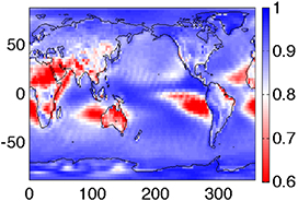
Figure 4.14. Map of the global distribution (in geographical coordinates) of the fraction (color scale is on the right) of wet to total deposition of 10Be, modeled with the ECHAM5-HAM general circulation model. Reproduced from Heikkilä et al. (2013), CC BY 3.0.
Download figure:
Standard image High-resolution imageHowever, over the Greenland and Antarctica ice sheets, dry deposition could play an important role. It was demonstrated (Figure 1 in Field et al. 2006) that at least from some areas, 10Be surface flux due to dry deposition can substantially exceed the contribution from wet deposition. For most regions, it is logical that dry deposition of cosmogenic isotopes is a minor sink, because the isotopes are produced in the middle atmosphere rather than at the surface. Due to the importance of wet deposition, sulfate deposition patterns correlate with precipitation: higher deposition is observed in the midlatitude storm tracks and tropical regions, and very low deposition fluxes are observed over the Sahara Desert and polar regions (Tost et al. 2007; Vet et al. 2014). Sulfate deposition maps are affected mainly by tropospheric transport rather than stratospheric transport, due to the large surface emissions of short-lived species. A better analogy for cosmogenic isotope deposition would be modeling studies that investigated deposition changes after stratospheric injections of SO2, in cases of geoengineering (Visioni et al. 2018; Kravitz et al. 2009) or volcanic eruptions (Marshall et al. 2018). The deposition response from stratospheric inputs of SO2 is largest in the midlatitudes of both hemispheres (Figure 4.15).
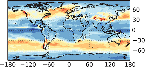
Figure 4.15. Zonal mean sulfate (kg SO4 km−2) deposited during the five years after the Tambora volcanic eruption in 1815 April. The results of the CESM1(WACCM) model are shown. Reproduced from Marshall et al. (2018), CC BY 4.0.
Download figure:
Standard image High-resolution imageTrajectory studies have determined that the highest mass fluxes of stratospheric air to the troposphere are located in the midlatitude storm tracks, especially in the northern hemisphere (Škerlak et al. 2014). Stratospheric aerosols likely enter the troposphere in the midlatitudes (Section 4.3.3), and therefore are likely deposited in the midlatitudes while only a small part can be transported and deposited over the polar areas. The same conclusions are valid for isotopes in soluble particulate forms. The isotopes in gas form (e.g., 14CO), however, will be mostly removed by dry deposition because of lower solubility.
4.3.7. Isotope Distribution in the Atmosphere
The atmospheric transport of isotopes was investigated using different models ranging from box, 1D and 2D models, to the most sophisticated 3D global coupled atmosphere–ocean general circulation models (GCM). The zonal and annual mean climatological distribution of 10Be and 7Be was calculated (Heikkilä 2007) using the ECHAM-HAM GCM (Figure 4.16). The ECHAM-HAM GCM treats all relevant processes of isotope transport including advective transport, turbulent mixing, and dry and wet deposition. The simulated isotopes are considered primary particles attached to sulfate aerosols, which means that gravitational sedimentation and solubility are taken into account.
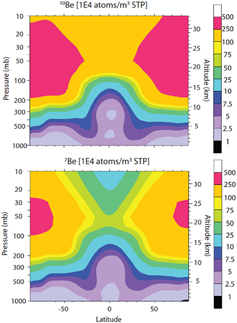
Figure 4.16. Altitude–latitude cross sections of zonal mean 10Be and 7Be number density at standard temperature and pressure (STP). © 2007 ETH-Zürich, reproduced from Heikkilä (2007) with permission of ETH-Zürich.
Download figure:
Standard image High-resolution imageThe altitude–latitude distributions of both isotopes are rather similar despite the substantial difference in decay time. The maximum is observed in the polar lower stratosphere where production by cosmic rays is maximized. The horizontal mixing of 7Be with about 50 days of decay time is less effective because the typical timescale of horizontal exchange in the stratosphere is about several years. Therefore, the horizontal gradient of the 7Be concentration in the stratosphere is larger than for 10Be, which is extremely passive in the stratosphere. In the troposphere, the concentrations of the considered isotopes are rather small and almost identical. This fact can be explained by the very fast removal of isotopes by wet deposition. The low abundance of these isotopes in the tropical upper troposphere is explained by intensive convective mixing, which moves up the air from planetary boundary layer with very low 7Be and 10Be concentrations. The stratosphere to troposphere transport is most pronounced over the middle latitudes, where the mixing is enhanced due to meteorological events in the troposphere (see Section 4.3.3). As mentioned in Section 4.3.5, the contribution of dry deposition is not important on a global scale and can be significant only in some specific arid regions, such as Greenland and Antarctica. Because long-lived isotopes (like 10Be) trapped in the ice cores are of great interest for the reconstruction of past solar activity, their transport to the ice-covered land regions and subsequent deposition there are more important than pure stratospheric transport. Figure 4.17 shows the distribution of 10Be and 7Be in the surface air simulated with ECHAM-HAM GCM (Heikkilä 2007).
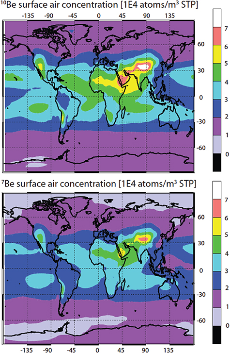
Figure 4.17. The 10Be (above) and 7Be (below) concentrations in the near-surface air. The color bars show the surface air concentration (104 atoms/m3) for the standard condition of temperature and pressure (STP). © 2007 ETH-Zürich, reproduced from Heikkilä (2007) with permission of ETH-Zürich.
Download figure:
Standard image High-resolution imageThe main features of the 10Be and 7Be geographical distribution are virtually the same; however, the absolute values of 7Be concentration are smaller, probably due to stronger decay during the stratosphere to troposphere transport. The maximum values of near-surface concentrations for the both isotopes appear over the middle latitudes, where the stratospheric air masses enter the troposphere. The minimum values are observed over areas with strong precipitation (e.g., Western Pacific) because of enhanced wet deposition and over high latitudes, where the isotopes are lost by decay during rather slow transport from the middle latitudes. Local peaks over North Africa, Saudi Arabia, and Tibet are mostly explained by weak precipitation and intensive transport form the stratosphere; however, the increase of tropospheric isotope production with height can also play some role (some localized spikes appear over the Rocky Mountains and Andes). The surface mixing ratio does not provide information about the origin of the isotope, which is important to properly attribute the observed variability. This information can be extracted from model runs especially designed to elucidate the location where the isotope in the surface air was produced. Such simulations were carried out (Heikkilä et al. 2009) using the ECHAM-HAM GCM, and the obtained results are shown in Figure 4.18.

Figure 4.18. Correspondence between the 10Be production and deposition regions. For example: 64% of the 10Be produced in the latitude band 60°–90°N is deposited over the 30°–60°N area. Reproduced from Heikkilä et al. (2009), CC BY 3.0.
Download figure:
Standard image High-resolution imageThis figure demonstrates very localized downward propagation of 10Be, when about 60% of the produced isotope is deposited in the same latitudinal band. The obtained interhemispheric exchange is also very slow compared to the deposition lifetime: only about 20% of the 10Be produced in the northern hemisphere propagates to the southern tropical latitudes. The obtained results also show that most of the 10Be produced in the stratosphere (90%) is deposited outside the polar caps, which are the most interesting locations for studies of the historical variability of solar activity. However, Heikkilä et al. (2009) also stated that the stratospheric source is responsible for about 65% of the total deposition in the polar areas.
4.3.8. Solar Influence on the Isotope Distribution
Because the stratosphere is the dominant source region for 10Be in polar surface air, the solar influence on 10Be production will be imprinted onto polar surface archives. The connection between solar activity and 10Be deposition in ice can be confirmed using both observations (e.g., Beer et al. 1990; Bard et al. 1997) and models (e.g., Heikkilä et al. 2008), which showed that some of the atmospheric transport variability do not play a dramatic role. Features of atmospheric transport can be illustrated using the simulated response of 10Be deposition to short-term explosive events on the solar surface. The consequences of one such extreme event in 775 CE was simulated with the chemistry-climate model SOCOL (Sukhodolov et al. 2017). The simulated and measured 10Be deposition fluxes are depicted in Figure 4.19.
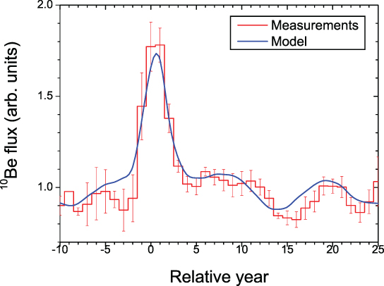
Figure 4.19. Annual depositional fluxes of 10Be (10−2 atoms/cm2/s) for the period around 775 CE. Red lines with error bars depict the mean of the measured data for four considered sites, while blue lines depict the ensemble mean of the simulation results. Figure is provided by T. Sukhodolov. More details are available from Sukhodolov et al. (2017).
Download figure:
Standard image High-resolution imageThe simulations were performed using a simplified treatment of wet and dry deposition. In addition, the produced 10Be was transported without attachment to the sulfur aerosol. The simulated 11 year variability and timing of the 10Be spike after the event are in good agreement with observations,which confirmed earlier conclusions about the small influence of gravitational sedimentation on the isotope deposition flux (Junge 1963; Lal & Peters 1967), at least in the absence of powerful volcanic eruptions. The mean time for the transport from the stratosphere was estimated as 1–2 years, which is in general agreement with the typical transport time discussed earlier. More accurate estimates of the time for the transport from the stratosphere are difficult because of the uncertainties in the observational data and the many processes involved in the transport and deposition of 10Be. This problem can be illustrated by comparing the transport time of sulfate aerosol after powerful volcanic eruptions simulated with different models to the measured deposition of the sulfate to ice. The comparison is relevant because of the close connection between 10Be and sulfate aerosol distribution, transport, and deposition.
Figure 4.20 illustrates the comparison of the observed sulfate deposition over Antarctica and Greenland after the Tambora eruption in 1815 April with four different model results (Marshall et al. 2018). The first traces of enhanced sulfate appear in the observations about six to seven months after the eruption in both locations, which is rather fast considering the distance from the tropics, where the eruption took place. The maximum values of the deposited sulfate are reached after about 1 year in both hemispheres if the second spike after 20 months is not considered. In the MAECHAM5-HAM, model the arrival of enhanced sulfate to the polar regions is even faster (around three to five months), especially for Antarctica. The SOCOL-AER simulation of the sulfate arrival time is similar to the observations, but the shape of the spikes is smoother. Two other models demonstrate rather different behaviors, showing smaller deposition magnitudes and a shift in the time response.

Figure 4.20. Simulated area-mean volcanic sulfate deposition (kg SO4 km−2 month−1) to the (a) Antarctic ice sheet and (b) Greenland ice sheet for each model (colors). Each ice-sheet mean is defined by taking an area-weighted mean of the grid boxes in the appropriate regions once a land–sea mask has been applied. Solid lines mark the ensemble mean, and shading is 1 standard deviation. (c) Deposition fluxes from two monthly resolved ice cores (DIV2010 from Antarctica and D4 from Greenland). The scale is reduced in (c). The gray triangles mark the start of the eruption (1815 April 1). Reproduced from Marshall et al. (2018), CC BY 4.0.
Download figure:
Standard image High-resolution imageThis example illustrates that model uncertainties in the stratosphere-to-troposphere transport of aerosols remain a challenge. Accurate simulations of the 10Be atmospheric transport and deposition require further improvements to all relevant model components.
4.3.9. Isotope Response to Climate Change and Volcanic Eruptions
Another problem related to the application of isotopes for the estimation of past solar activity is the influence of atmospheric circulation and deposition parameters. It is well known that greenhouse gases affect the atmospheric temperature and circulation, with implications for the water cycle, convection, and cloud properties. For the recent past, the magnitude of this impact is suggested to be small, in part because the climate changes during the preindustrial period were not too strong. For the distant past and future, the isotope deposition response to climate changes can be estimated only using state-of-the-art models, because of the lack of reliable observations. The Maunder minimum of solar activity and a warmer climate in the future are two interesting cases to consider. The deposition of 10Be during the Maunder minimum was simulated by Heikkilä et al. (2008) using the ECHAM-HAM model. They introduce a 32% 10Be production increase for this period and compared the deposition flux increase with this value. For the global mean deposition flux, 8% (1/4 of the production increase) was attributed to a colder climate, weaker stratospheric transport, and a different hydrological cycle. However, Figure 4.21 shows that over Antarctica and Greenland (not shown), the relative increase of 10Be deposition can exceed 100%, which means that the influence of climate can dominate in case of strong changes in different climate states.
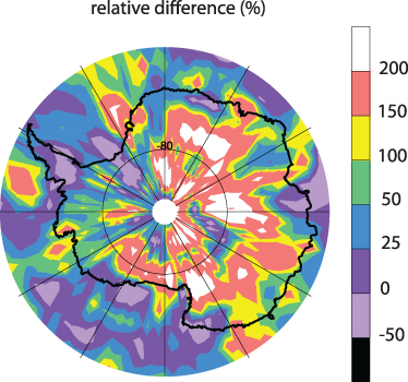
Figure 4.21. Difference between modeled 10Be depositions during the Maunder Minimum and the present day in Antarctica in relative (%) units. Reproduced from Heikkilä et al. (2008), CC BY 3.0.
Download figure:
Standard image High-resolution imageBecause the deposition flux over ice sheets is important for the study of past solar activity, the assumption about the negligible influence of climate change on isotope composition needs to be further investigated. If the emission of greenhouse gases continue above preindustrial levels, the future climate will be warmer and characterized by a stronger meridional circulation (e.g., Li et al. 2008). The response of the 10Be concentration in snow to climate regime switches was evaluated by Field et al. (2006) using the GISS GCM. They compared present-day simulations with simulations of a warmer climate caused by CO2 doubling, as well as a simulation with a colder climate during the Younger Dryas. Figure 4.22 illustrates the influence of climate warming on the 10Be concentration in snow in the polar areas. Intensification of meridional circulation in the stratosphere leads to the faster removal of 10Be from the production area in the lower stratosphere. Potentially, it could result in tropospheric 10Be enhancement, but as stated in Field et al. (2006), the intensification of hydrological cycles removes more 10Be, compensating for the influence of circulation changes. This effect leads to a decrease of 10Be in snow and more intensive snow accumulation over Antarctica and Greenland by up to 50%. It was concluded in Field et al. (2006) that 10Be changes due to warmer climate are driven by global-scale changes of the hydrological cycle and not by the changes in local deposition.

Figure 4.22. Percent change in 10Be snow concentration for the 2xCO2 simulation relative to the control run over (a) Greenland and (b) Antarctica. Results (courtesy of G. Schmidt) are based on the model (Field et al. 2006; Veeder 2009). Copyright (2009) by Columbia University Press. Reproduced with permission of Columbia University Press via Copyright Clearance Center.
Download figure:
Standard image High-resolution imageAnother interesting aspect of the problem is the influence of volcanic eruptions on the isotope concentration in ice. They can be connected due to the modulation of sulfate aerosol loading by powerful volcanic eruptions leading to changes in the vertical and horizontal transport of isotopes attached to sulfate aerosol particles. These changes could be important because the increased size of aerosol particles after volcanic eruption can substantially intensify downward transport, and their radiative effects can suppress the hydrological cycle (e.g., Grinsted et al. 2007). The correlation between 10Be and sulfate deposition in the observations was discussed in Baroni et al. (2011, 2019). They found a simultaneous increase of sulfate and 10Be in cores from two Antarctic sites, Vostok and Concordia, after the powerful volcanic eruptions from Agung and Pinatubo. High-resolution ice-core records from several sites in Antarctica have now been extended back to 887 CE, and among 26 volcanic eruptions studied, 14 have been confirmed to have an increase in 10Be concentration related to stratospheric volcanic eruptions (Baroni et al. 2019). A detailed explanation of the obtained correlation is difficult to obtain from pure observational data because many processes are involved in the primary signal transformation. The study of the 10Be deposition response to volcanic eruptions was carried out in Field et al. (2006) using the GISS GCM. In their model, only the influence of the colder climate was considered, because the model was not able to treat gravitational sedimentation and the potential effect of volcanic eruption on 10Be scavenging. The obtained results showed a small (about 6%) influence of volcanic eruptions on stratosphere–troposphere exchange and the tropospheric concentration of 10Be. Figure 4.23 illustrates the changes of 10Be in snow for Antarctica. For this region, the suppressed hydrological cycle leads to lower accumulation rates and reduced wet deposition with almost no changes in dry deposition, resulting in an up to 20% increase of the 10Be concentration in snow.
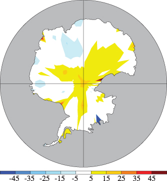
Figure 4.23. Percent change in 10Be snow concentration for the peak years of the volcanic simulation relative to the 100 year mean. Results (courtesy of G. Schmidt) are based on the model (Field et al. 2006; Veeder 2009). Copyright (2009) by Columbia University Press. Reproduced with permission of Columbia University Press via Copyright Clearance Center.
Download figure:
Standard image High-resolution imageHowever, a change in accumulation rates would also affect the concentration of other proxies recorded in the snow (e.g., sodium, magnesium which are proxies of marine sources) and no obvious change is observed after volcanic eruptions. The study of 14 volcanic periods from Antarctic ice cores covering the last millennium shows that the increase in 10Be concentration varies from 14% to 112%. This large range depends upon the volcanic source parameters (amount of SO2 emitted, altitude reached in the stratosphere, location of the volcano, etc.) and the preservation of the signal in the ice. These results agree with the analysis of observational data by Baroni et al. (2011); however, the description of the involved mechanisms differs. Baroni et al. (2011, 2019) suggested that the large amount of sulfate aerosols formed in the stratosphere on a short timescale after a volcanic eruption would accelerate their sedimentation, dragging 10Be atoms along in their path. The difference with Field et al. (2006), who claimed that hydrological processes in the troposphere are more important, can be related to the simplified treatment of volcanic aerosol by Field et al. (2006) and needs to be addressed in the future with proper models.
4.4. Isotope Archiving in Ice Cores
Mélanie Baroni
4.4.1. Archiving of 10Be
Impact of Stratospheric Volcanic Eruptions
Stratospheric volcanic eruptions can increase the concentration of 10Be in ice cores by up to 112% (Baroni et al. 2019) over one to three years. On average, the increase in the 10Be concentration is 56% ± 30% (Baroni et al. 2019), calculated from 14 volcanic periods recorded in different ice cores of the High Antarctic Plateau over the last millennium. For comparison, the 994 CE and the 775 CE SEP events induced, respectively, a 50% and 80%–150% increases in the 10Be concentration in ice cores from Antarctica and Greenland (Mekhaldi et al. 2015; Miyake et al. 2019, 2015; Sigl et al. 2015). A stratospheric volcanic eruption can therefore reproduce a 10Be signal mimicking an SEP event. Thus, it is necessary to compare the concentrations of 10Be and of sulfate, a proxy for volcanic eruptions, in the same ice core, to verify the solar or volcanic origin of a 10Be peak (see Figure 4.24). Another verification consists in looking at 14C tree-ring data that are not, a priori, affected by volcanic eruptions. Indeed, the amount of CO2 emitted by volcanoes is negligible compared to the atmospheric reservoir. It is possible to apply a correction for the volcanic disturbance using the slope of the linear regression between the 10Be and sulfate concentrations if they were determined from the same samples (red line, Figure 4.24; Baroni et al. 2011).
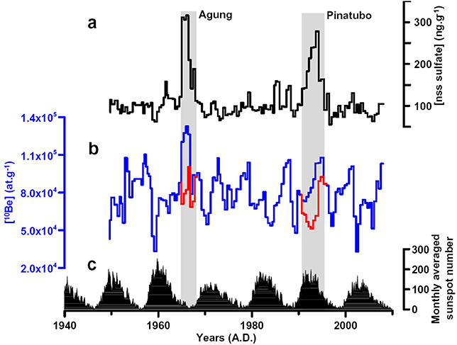
Figure 4.24. Variability of the non-sea-salt sulfate concentration (nss sulfate) in the Vostok Antarctic ice core (panel a), raw 10Be concentration in the same ice core (panel b, blue curve), and the 10Be concentration corrected for the volcanic contribution (panel b, red curve) for the Agung and Pinatubo eruptions using the relationship between the concentrations of 10Be and volcanic nss sulfate, and the monthly averaged sunspot number (panel c). Reprinted from Baroni et al. (2011), copyright (2011), with permission from Elsevier.
Download figure:
Standard image High-resolution imageThe mechanism responsible for the impact of stratospheric volcanic eruption on 10Be deposition involves the microphysics of aerosols. Volcanic eruptions generate large amounts of sulfate aerosols on a short timescale, accelerating their gravitational sedimentation because of a higher collision rate, making larger aerosols than in nonvolcanic conditions (e.g., Pinto et al. 1989; Timmreck 2012). It would also increase the sedimentation of 10Be atoms as they attach to aerosols to settle at Earth's surface (Baroni et al. 2011, 2019). However, this is only part of the story—the volcanic imprint is so visible in 10Be ice-core records because the 10Be is mostly produced in the polar stratosphere, between 10 km and 15 km altitude (Delaygue et al. 2015; Poluianov et al. 2016) and because the 10Be snow signal is controlled by stratospheric intrusions even in nonvolcanic conditions, at least on the High Antarctic Plateau. For example, the 10Be snow/ice signal at Dome C and the South Pole, both located on the High Antarctic Plateau, is controlled by 2%–5% of stratospheric intrusions (Baroni et al. 2019; Hill-Falkenthal et al. 2013; Raisbeck et al. 1981). Any change in the aerosol load in the stratosphere would be seen in 10Be time series.
Climatic or System Effects
Several studies report "climatic" or "system" effects to explain part of the 10Be ice-core signal which is not related to modulation of its production in the atmosphere (e.g., Baroni et al. 2011; Beer et al. 1992; Miyake et al. 2019; Pedro et al. 2006, 2011; Winkler et al. 2013).
For example, comparisons are made with the water δ18O values, which is an indicator of the local temperature that can be related to a change in moisture sources and finally on dry versus wet deposition (see Section 5.3). The cross-correlation coefficient between 10Be and δ18O is 0.57 at a high-accumulation-rate site such as Law Dome (Antarctica; Pedro et al. 2006) and 0.32 at a low-accumulation-rate site such as Vostok (Winkler et al. 2013), where dry deposition dominates. This can affect the 10Be concentration.
A relationship between the concentrations of sodium (Na+) and 10Be has also been observed at several sites in Antarctica, Dome C, Dome Fuji, and Law Dome (Baroni et al. 2011; Miyake et al. 2019; Pedro et al. 2011). Sodium is a sea salt, found as an aerosol particle, originating from the ocean and transported inland in the troposphere. The cross-correlation between the concentrations of 10Be and Na+ over the last 60 years, at Vostok, is 0.51 (Baroni et al. 2011), and a similar value is found at Dome Fuji at the time of the 994 CE event (Figure 4.25; Miyake et al. 2019). The mechanism explaining the relationship between the concentrations of 10Be and Na+ is not yet identified, but at Vostok, both vary according to a cyclicity of a 3–7 year interannual variability. This cyclicity is found in different modes of atmospheric circulation, such as the Antarctic Oscillation, the Antarctic Circumpolar Wave, or the Southern Annular Mode (Baroni et al. 2011). The modulation of atmospheric circulation in the troposphere might explain this relationship, but more investigations are needed in the future.
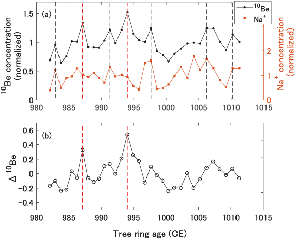
Figure 4.25. Panel a: comparison between 10Be and Na+ data around 994 CE. Panel b: Δ10Be values (see Equation (4.7)). Adopted from Miyake et al. 2019.
Download figure:
Standard image High-resolution imageHowever, whatever the mechanism is, it is possible to apply a correction to the 10Be signal to remove part of the "system effect" (Miyake et al. 2019). Using the linear regression between the normalized concentrations of 10Be and Na+, the relative production variability of 10Be, called Δ10Be (Figure 4.25), can be calculated:

where 10Be(t) is the normalized 10Be concentration at time t, Na(t) is the "normalized Na+ concentration," and C(t) is the regression line between the normalized 10Be and Na+ concentrations. This "system effect" correction allowed the strength of the 994 CE event recorded at Dome Fuji (Miyake et al. 2019) to be better emphasized.
4.4.2. Archiving of 36Cl
Anthropogenic 36Cl from Nuclear Bomb Tests
In natural conditions, 36Cl is produced in the atmosphere through cosmic-ray-induced spallation of 40Ar nuclei (Poluianov et al. 2016). Aside from its natural source, anthropogenic 36Cl has also been produced through capture by 35Cl from the sea salt (sodium chloride NaCl) of thermal neutrons emitted during the marine nuclear bomb tests (Bentley et al. 1982; Elmore et al. 1982; Heikkilä et al. 2009) from the 1950s to the 1970s. Other nuclides such as cesium-137 (137Cs) or tritium (3H) were mainly produced during atmospheric and ground nuclear tests.
The intensity of these marine nuclear tests made 36Cl reach the stratosphere, mainly in the gaseous form H36Cl (Zerle et al. 1997), then be distributed across the globe, and finally transferred to the troposphere. Consequently, the 36Cl bomb pulse can be observed at all latitudes including Greenland and Antarctica (Figure 4.26; Delmas et al. 2004; Elmore et al. 1982; Heikkilä et al. 2009; Synal et al. 1990).

Figure 4.26. The measured (upper panel) and modeled (middle panel) peaks of 36Cl deposition fluxes at eight ice-core sites. The vertical lines in the lower panel show the bomb test input of 36Cl. Reproduced from Heikkilä et al. (2009), CC BY 3.0.
Download figure:
Standard image High-resolution imageApproximately 80 kg of 36Cl were injected into the stratosphere between 1952 and 1971 (Heikkilä et al. 2009; Synal et al. 1990), resulting in a 36Cl flux at low-latitude glaciers of Greenland and Antarctica, 100–1000 times higher than the natural prebomb 36Cl fluxes (Figure 4.26). As a result, SEP events occurring during that time period, such as the hard-spectrum one of 1956 February 23, would be hardly possible to detect. Since the end of the marine nuclear bomb tests, prebomb 36Cl levels have nearly recovered in ice cores, in the 1980s (Elmore et al. 1982; Heikkilä et al. 2009), opening prospects for using36Cl to detect SEPs in the future.
Mobility of 36Cl in the Snowpack
Prebomb 36Cl level has still not recovered in 1998, at Vostok, in Antarctica (Figure 4.27; Delmas et al. 2004). This was explained by the mobility of 36Cl in its gaseous form (H36Cl), in firn, at this low-accumulation site, which was evidenced when comparing 36Cl with 137Cs measured in the same snow pit (see Figure 4.27). Even though 137Cs was produced during atmospheric nuclear tests and 36Cl was produced during the marine ones, they can be compared because the tests were performed during the same period. Anthropogenic 36Cl peaks should be in phase with those of 137Cs identified in 1955 and 1965, but at Vostok, the anthropogenic 36Cl migrates toward the surface. The mobility of 36Cl is not observed at the Dye-3 and NGRIP sites in Greenland and is limited at Berkner Island in Antarctica, where 36Cl deposited as gaseous H36Cl and particulate Na36Cl are both well preserved (see Figure 4.26). This could be explained by the higher accumulation rates for these sites compared to Vostok (Delmas et al. 2004; Heikkilä et al. 2009).
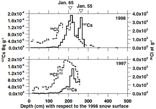
Figure 4.27. Fallout of 137Cs (solid lines, left scale) and 36Cl (dashed lines, right scale) at the Vostok site as a function of depth (1997 and 1998 snow pits are shown on the bottom and top panels, respectively). The depth of the 1997 samples has been shifted by −7 cm to take into account the 1 yr time lag between the two sampling dates. Reproduced from Delmas et al. (2004), CC BY 4.0.
Download figure:
Standard image High-resolution imageLow-accumulation sites
( water equivalent/year) are also affected
by a significant loss of chlorine during interglacial periods. The loss can be up to
60% or 80% at Dome C and Vostok (Antarctica), respectively (Röthlisberger et al.
2003; Wagnon et
al. 1999). This
would impact the 36Cl/10Be ratio used to constrain the energy
spectra of SEPs. These peculiarities have to be taken into account for a better
interpretation of 36Cl ice-core data.
water equivalent/year) are also affected
by a significant loss of chlorine during interglacial periods. The loss can be up to
60% or 80% at Dome C and Vostok (Antarctica), respectively (Röthlisberger et al.
2003; Wagnon et
al. 1999). This
would impact the 36Cl/10Be ratio used to constrain the energy
spectra of SEPs. These peculiarities have to be taken into account for a better
interpretation of 36Cl ice-core data.
4.5. Lunar Archives
A. J. Timothy Jull And Stepan Poluianov
4.5.1. Cosmogenic Radionuclides on the Moon
The Moon has no magnetic field, and therefore its surface is bombarded with the full
flux of GCRs and SEPs, as well as solar wind. While more energetic cosmic rays can
produce cosmogenic isotopes inside the upper layer of the lunar soil/rock, ions of
solar wind can be implanted on the surface. A considerable number of radionuclides
have been used to estimate GCR fluxes on the Moon. Radioisotopes in lunar samples that
have been measured and that can be used to study SEP fluxes in the past include
22Na (T1/2 = 2.6 yr; Fruchter et al. 1976), 39Ar
(T1/2 = 269 yr; Fireman et al. 1970; Stoenner et al. 1970), 14C
(T1/2 = 5730 yr; Begemann et al. 1972; Boeckl 1972; Jull et al. 1995, 1998), 59Ni
(T1/2 = 76,000 yr; Lanzerotti et al. 1973), 41Ca
(T1/2 = 0.1 Myr; Nishiizumi et al. 1997; Fink et al. 1998), 81Kr
(T1/2 = 0.2 Myr; Reedy & Marti 1991), 36Cl
(t1/2 = 0.3 Myr; Nishiizumi et al. 1984, 1989), 26Al
(T1/2 = 0.710 Myr; Fruchter et al. 1976; Kohl et al. 1978; Nishiizumi et al. 1984, 2009), 10Be
(T1/2 = 1.38 Myr; Nishiizumi et al. 1984, 2009), and 53Mn
(T1/2 = 3.7 Myr; Kohl et al. 1978; Nishiizumi et al. 1983; Russ & Emerson
1980). On the Moon,
most of these radionuclides such as 14C and 10Be are primarily
produced in rocks by high-energy spallation reactions on different target elements.
SEPs are less energetic, with energies of tens to hundreds of megaelectronvolts, which
is still sufficient to induce spallation reactions. They have a variable flux,
typically around 100 particles cm−2 s−1
( ). Studies of depth profiles in the near
surface (<1–2 cm) have been successfully used to derive SEP fluxes in cases where
production rates are well known, such as on the lunar surface (Finkel et al. 1971; Fruchter et al. 1976; Fink et al. 1998; Jull et al. 1998; Nishiizumi et al.
2009). Constraints
on the temporal variability of the SEP flux have also been determined by comparison of
radionuclides with different half-lives (e.g., Nishiizumi et al. 1984; Reedy 1998; Eugster et al. 2006; Nishiizumi et al. 2009; Reedy 2012a).
). Studies of depth profiles in the near
surface (<1–2 cm) have been successfully used to derive SEP fluxes in cases where
production rates are well known, such as on the lunar surface (Finkel et al. 1971; Fruchter et al. 1976; Fink et al. 1998; Jull et al. 1998; Nishiizumi et al.
2009). Constraints
on the temporal variability of the SEP flux have also been determined by comparison of
radionuclides with different half-lives (e.g., Nishiizumi et al. 1984; Reedy 1998; Eugster et al. 2006; Nishiizumi et al. 2009; Reedy 2012a).
SEP effects are important in lunar samples, but because SEP effects are rarely observed in meteorites (Nishiizumi et al. 1990, 2014), the cosmogenic nuclide record in lunar samples is unique because they provide a continuous record of GCR and SEP intensities. Lunar cores are very useful in studies of the production of nuclides by GCR particles in planetary surfaces. Lunar samples also contain good records of SEP effects and variations of SEP fluxes in the past (Reedy 1980, 1998; Reedy & Marti 1991).
Cosmogenic isotopes can also be used to identify solar-wind implanted components in lunar rocks, as shown in the case of 14C (Jull et al. 1995, 2000) and to some extent, 10Be (Nishiizumi & Caffee 2001).
Generally, lunar rocks and soil-core samples are considered to be excellent recorders of GCR and SEP effects (Reedy et al. 1983; Reedy 1998). Their long residence times on a stable surface integrate the past irradiation of the rocks and core samples. Spallation-produced 14C, 10Be and other radionuclides are important for determining solar (SEP) and galactic cosmic-ray production rates. We can do this by comparing flux estimates derived from radioisotopes, which have different half-lives, spanning several orders of magnitude in time (Jull et al. 1998; Fink et al. 1998; Table 4.3).
Table 4.3. Solar-proton Spectral Shape (Exponent in Rigidity, R0) and Omnidirectional Fluences (in cm−2 s−1) above Given Energies (10, 30, 60, and 100 MeV, Denoted F10, F30, F60, and F100, Respectively) Determined from Lunar Sample Data Using Different Isotopes
| Time Range | Nuclide | References | R0 (MV) | F10 | F30 | F60 | F100 |
|---|---|---|---|---|---|---|---|
| 1954–2013 | Direct | Table 2.2 | 60–100 | ∼127 | 31 | ∼10 | — |
| 1954–1964 | 22Na, 55Fe | (Reedy 1977, 1998; Sisterson et al. 1996) | 100 | 227 | ∼82 | ∼35 | ∼26 |
| 104 yr | 14C | (Jull et al. 1998) | 113 | 103 | 42 | 17 | 7 |
| 105 yr | 41Ca | (Klein et al. 1990) | 70 | 120 | 28 | 7 | 1.5 |
| (Fink et al. 1998) | 80 | 200 | 56 | 16 | 4 | ||
| 3 × 10⁵ yr | 81Kr | (Reedy & Marti 1991) | ∼85 | — | — | 14 | 4 |
| 5 × 10⁵ yr | 36Cl | (Nishiizumi et al. 2009) | ∼75 | 100 | 26 | 7 | 2 |
| (Nishiizumi et al. 2009) | 70 | 196 | 46 | 11 | — | ||
| 106 yr | 26Al | (Kohl et al. 1978) | 100 | 70 | 25 | 9 | 3 |
| (Nishiizumi et al. 1988) | 70 | 150 | 35 | 8 | — | ||
| 2 × 10⁶ yr | 10Be, 26Al | (Nishiizumi et al. 2009) | 75 | 100 | 26 | 7 | 2 |
| (Michel et al. 1996) | 125 | 55 | 24 | 11 | 5 | ||
| (Fink et al. 1998) | 100 | 89 | 32 | 12 | 4 | ||
| (Nishiizumi et al. 2009) | 90 | 73 | 24 | 8 | ∼2 | ||
| 5 × 10⁷ yr | 53Mn | (Kohl et al. 1978) | 100 | 70 | 25 | 9 | 3 |
| ∼2 × 10⁶ yr | 21Ne, 22Ne, 38Ar | (Rao et al. 1994) | 80–90 | 58–87 | ∼22 | ∼7 | ∼2 |
Note. Values on the top row represent data from direct spaceborne measurements (Section 2.2).
4.5.2. Near-surface Components of Cosmogenic and Radiogenic Nuclides
Without a shielding atmosphere and magnetic field, all charged particles can reach the lunar surface. In addition to galactic and solar energetic particles, discussed in Section 2.2, there is also a population of less energetic (and not always fully ionized) solar wind particles. The solar wind consists of ions entrained in the solar magnetic field, with a flux of protons of 1.6–2 × 10⁸ p cm−2 s−1 (Geiss et al. 1970). Because the solar wind impinges on the lunar surface most of the time, except when the Moon is in the terrestrial magnetic field (Winglee & Harnett 2007), we expect that these ions should be implanted into lunar surface materials. Such effects have been studied by many researchers for radionuclides such as 14C (Fireman et al. 1977; Fireman 1978; Jull et al. 1995, 2000), 10Be (Nishiizumi & Caffee 2001), and noble gases (Wieler 1998). There is also evidence for directly implanted solar 14C in lunar soil, from either solar wind or solar flares (Fireman et al. 1977; Fireman 1978; Jull et al. 1995, 2000; Lal et al. 2007). The effect of continuous solar-wind implantation and sputtering on the lunar surface also causes the erosion and remobilization of material (Killen & Ip 1999; Wurz et al. 2007). A number of studies have shown that sputtering effects on the lunar surface (e.g., Jull et al. 1980; Kitts et al. 2003) cause compositional changes.
The SEP flux were estimated from recent spacecraft measurements (see Section 2.2.3) and summarized in
Table 2.2. As terrestrial
cosmogenic data suggest, there have been no SEP events with the fluence
 over the last 11,000 years see Usoskin et
al. (2006) and Usoskin
& Kovaltsov (2012).
over the last 11,000 years see Usoskin et
al. (2006) and Usoskin
& Kovaltsov (2012).
4.5.3. Lunar Archives Relevant for Solar and Galactic Cosmic-ray Records
The first lunar landing occurred on 1969 July 20. The Apollo 11 mission returned some bulk soil samples and rocks. Subsequent Apollo missions between 1969 and 1972 returned about 382 kg of lunar samples in total, including 265.6 kg of rocks (>1 cm; Heiken et al. 1991). Six of the seven missions landed and returned samples from the Moon. One mission, Apollo 13, had to be aborted due to a technical problem. The later missions (Apollo 14–17) were increasingly oriented to the geology of the Moon, and Apollo 17 included a geologist as one of the astronauts (Harrison Schmitt). These are well documented, and there is extensive literature available at https://curator.jsc.nasa.gov/lunar/, which gives detailed information and access to a compendium of information on all lunar samples. Detailed records of astronaut observations and discussions on the lunar surface (Figure 4.28) and sample collection are also available at the Apollo lunar journal site, https://www.hq.nasa.gov/alsj/main.html. There are also some much smaller samples collected as part of the Soviet automatic landers Luna 16, 20, and 24, which collected a total of 321 g of material in three small cores. There was also a fourth lander (Luna 23), but it failed on landing. Detailed information is also available at the NASA lunar sample compendium site, https://curator.jsc.nasa.gov/lunar/lsc/.

Figure 4.28. Photograph from the Apollo 17 mission, showing astronaut Harrison Schmitt standing next to a large split boulder (NASA photo AS17-140-21496). Courtesy of NASA.
Download figure:
Standard image High-resolution image4.5.4. Past Lunar Investigations into SEP and GCR Production
Lunar Cores
Of the 25 cores of lunar soil taken during the Apollo missions, 16 have so far been studied for cosmogenic nuclides. Many of the cores studied show surface disturbance either during sampling or transport. Two types of cores were collected. In all missions, short drive tubes of up to ∼30 cm length were collected, and "double-drive cores" were used for the Apollo 15, 16, and 17 missions (Meyer 2007d), consisting of tubes ∼34 cm long, which coupled together collected up to 68 cm of core (see Figure 4.29). For Apollo 15–17, longer "deep drive cores" were also collected, which were about 242, 224, and 300 cm in length, respectively (Meyer 2007a, 2007b, 2007c). The best core appears to be the Apollo 15 deep-drill core, 15008/7 (Fruchter et al. 1976; Nishiizumi et al. 1984, 1997; Jull et al. 1998), which preserves the best record of solar cosmic-ray signal at the surface. According to Allton & Waltz (1980, p. 1475) "the Apollo 15 drill core was completely filled and its scale is straightforward and accurately represents in situ lunar conditions." Figure 4.29 shows the rather difficult process of setting up the deep-drill core.

Figure 4.29. Photograph of the Apollo 15 commander setting up the deep-drill core during Apollo 15 (NASA photo AS15-87-11847). Courtesy of NASA.
Download figure:
Standard image High-resolution imageA summary of all lunar cores with references is given in Table 4.4.
Table 4.4. Lunar Core Samples Recovered During Apollo Missions
| Core | Length (cm) | Weight (g) | References and Notes | |
|---|---|---|---|---|
| 10004 | Single | 13.5 | 44.8 | Allton & Waltz (1980) |
| 10005 | Single | 10 | 53.4 | |
| 12026 | Single | 19.3 | 101.4 | |
| 12027 | Single | 17.4 | 80 | |
| 12025/12028 | A12 deep drill | 41 | 246.7 | |
| 12023/12024 | A12 core | 37 (from trench) | Not in core summary | |
| 14210/14211 | Double-drive core | 40 | 209.2 | 14210—full, 14211—not full, only 39.5 g |
| 14220 | Single core | 16.5 | 80.7 | |
| 14230 | Single core | 12.5 | 76.7 | |
| 15007/15008 | Double-drive core | 56.6 | 1278.4 | Many studies |
| 15009 | Single core | 30 | 622 | |
| 15010/15011 | Double-drive core | 55 | 1401.1 | Meyer (2007d) shows the complete core |
| 60009/60010 | Double-drive tube | 65.4 | 1395.1 | Fruchter et al. (1976), Meyer (2007d) |
| 64001/64002 | Double | 65.6 | 1336.4 | Top 20 cm disturbed (Meyer 2007d) |
| 68001/68002 | Double | 62.3 | 1424.2 | Binnie et al. (2019) |
| 69001 | Single | 27 | 558.4 | Unopened (Lofgren 2011) |
| 60001/60007 | Deep drill | 224 (195 recovered) | 1007.6 recovered | Fruchter et al. (1976) (top) 60005 has missing section. |
| 15006/15001 | Deep drill | 237.2 | 1333 | Fruchter et al. (1976), Meyer (2007c) |
| 76001 | Single | 34.5 | 711.6 | Jull et al. (1998) |
| 79001/79002 | Double drive | 51.3 | 1152.8 | |
| 70001/70009 | Deep drill | 300 | 1368.5 | (top) Fruchter et al. (1976), Meyer (2007c) |
| 70012 | Single | 28 | 485 | Found already open in LRL (Meyer 2009) |
| 73001/73002 | Double | 56 | 1239 | Unopened (Lofgren 2011) |
| 74001/74002 | Double | 68.2 | 1979.2 |
Note. Apollo Sample Catalogs Index, https://curator.jsc.nasa.gov/lunar/catalogs/index.cfm, Fruchter et al. (1976). LRL denotes Lunar Receiving Laboratory.
The shorter Apollo 15 core 15008/7 (Reedy & Nishiizumi 1998; Jull et al. 1998) as well as the deep-drill core preserve a good record of the SEP component. This can be seen in Figures 4.30 and 4.31. Figure 4.30 shows the deeper profile from the galactic component (GCR) for the 2 m core. A smooth curve of the SEP component in the top 5 g cm−2 can be seen in Figure 4.31, which shows the top 20 cm of the cores. However, Fruchter et al. (1976) noted that the deep-drill stem (15006) showed disturbance in the top 20 cm for 26Al.
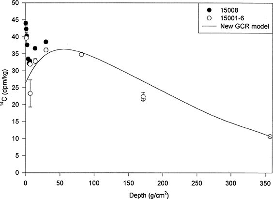
Figure 4.30. Detail of 14C in the top portion of the lunar core 15008 and the Apollo 15 deep-drill core (15001/6). Reprinted from Jull et al. (1998), copyright (1998), with permission from Elsevier.
Download figure:
Standard image High-resolution image
Figure 4.31.
14C concentration (dpm kg−1) in the top portion of lunar
cores 15008 (solid circles) and 15006 (open circles). The best-fit calculations
for the combined effect of SEP and GCR, using the SEP production for a rigidity
parameter R0 of 110 MV with flux
 of 108 p cm−2
s−1. The calculated GCR curve is also plotted as the dashed line.
Reprinted from Jull et al. (1998), copyright (1998), with
permission from Elsevier.
of 108 p cm−2
s−1. The calculated GCR curve is also plotted as the dashed line.
Reprinted from Jull et al. (1998), copyright (1998), with
permission from Elsevier.
Download figure:
Standard image High-resolution imageApart from the very surface of the Apollo 15 core, Russ et al. (1972) and Pepin et al. (1974) showed that cosmic-ray-produced spallation nuclides are all smooth functions of depth. This indicates that the depositional history of the drill core is coherent and relatively simple. Bogard et al. (1973) and Bogard & Hirsch (1975) found that noble-gas solar-wind components can be documented throughout the length of the core. Bogard et al. (1973) showed that 4He and 4He/3He were relatively constant. These authors concluded that the Apollo 15 core represents the best sampling of a deep core on the Moon to date.
Disturbed Cores
However, other cores show different disturbances. In addition to the Apollo 15 deep-drill core, one of the most studied cores from the Moon is the Apollo 16 double-drive tube core (∼60 cm) 60009/60010, which has one of the best records of SEP and GCR effects, as well as track and other studies (e.g., Nishiizumi et al. 1979). Fruchter et al. (1976, 1982) and Nishiizumi et al. (1979) measured the SEP- and GCR-produced activity of 22Na, 26Al, and 53Mn. There is some disturbance at the top of the core, from lunar gardening, although (Fruchter et al. 1976) noted that the 22Na profile appeared undisturbed. Evans et al. (1980) used this data to calculate a regolith accumulation rate of 1–2 cm Myr−1 in the downslope environment of this core. They also estimate that this must be in the last ∼10 Myr to affect the 53Mn signal. The Apollo 16 double-drive tube shows SEP 22Na and 26Al, but 26Al flattens at the top. 22Na indicates a loss of 1 cm. 26Al indicates centimeter-scale mixing over the mean life of 26Al. Fireman et al. (1973) reported data for the isotopic composition of 39Ar. Wieler et al. (1986) carefully studied the isotopic composition of noble gases in plagioclase separates and determined that the ratio of the Ne component from solar flares and the solar wind was distinctly different for the bottom of the Apollo 16 deep-drill core.
In contrast to the Apollo 15 deep-drill core and the Apollo 16 double-drive tube, the 224 cm long Apollo 16 deep-drill core (60001/7) shows several disturbances (Meyer & McCallister 1977; Meyer 2009). Some other cores show disturbances either due to transport, or to the core not being intact inside the core sleeve, with various explanations. In a more recent study of cores 68001/68002 (drive tube), Binnie et al. (2019) also found disturbance in the first few centimeters of the core, perhaps due to regolith mixing or upwarping of the material in the tube.
Lunar Rocks Used for Detailed SEP Studies
A number of lunar rocks have been studied in detail for cosmogenic nuclide records. These samples probably offer the best records of SEP effects, as they are only subjected to low levels of erosion, and the turnover effects evident in cores can be avoided.
Early studies were conducted on rock 12002 from the Apollo 12 site (Finkel et al. 1971), which included short-lived nuclides. In this study, the rock was carefully sliced and external surfaces ground off using a dental tool. The short-lived nuclides suggested high flux rates than longer-lived nuclides. Similar studies were also done in Wahlen et al. (1972) for the large ∼9 kg rock 14321 (known as "Big Bertha"), a clast-rich crystalline matrix breccia. Other measurements have been performed on rock 10017 (Shedlovsky et al. 1970), 14320 (Wahlen et al. 1972) and also rocks 74275, 68815, and 64455. Perhaps the most detailed studies were for rock 64455, a glass-coated impact melt rock that was used for detailed studies of solar cosmic-ray effects (Ryder & Norman 1980; Nishiizumi et al. 2009). The solar-facing surface, which showed micrometeorite impact pits, was used for this study. Detailed studies that refined the flux were conducted for rock 64455 (Nishiizumi et al. 2009). In this study, the rock was ground off with a dental tool in finer fractions than for 12002. The approach used for rock 68815 was to slice different sections (Meyer 2009) at the Johnson Space Center curatorial facility. The most comprehensive series of these studies are those on 68815 (Nishiizumi et al. 1988; Kohl et al. 1978; Rao et al. 1994; Jull et al. 1998). Detailed studies on 68815 show a good record of SEP components of 14C, 10Be, 26Al, 36Cl, and 53Mn (Figure 4.32). No SEP 10Be was observed in 68815, and it was argued (Nishiizumi et al. 1988) that this sets upper limits on SEP, using 10Be as an indicator of the energy range of the SEP flux. Similar studies have been done for rock 74275 (Fink et al. 1998; Jull et al. 2001), which generally followed the idea of the original 12002 studies (Finkel et al. 1971).
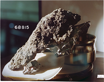
Figure 4.32. South face of lunar rock 68815 (NASA photo S72-41425), taken from the top of the rock shown in the field; see Figure 4.33. Courtesy of NASA.
Download figure:
Standard image High-resolution imageFor rock 64455, Nishiizumi et al. (2009) reported values of flux for
 of J = 24 p
cm−2 s−1
(
of J = 24 p
cm−2 s−1
( MV) for 26Al, but a higher
value of J = 46 p cm−2 s−1 (with a lower
R0 of 70 MV) for 36Cl. Their values appear
to be consistent with other records (shown in the table for this and other rocks)
that indicate that the SEP flux is on average higher during the last 0.5–1 Myr,
based on results from 14C (68815; Jull et al. 1998), 36Cl (64455 and 68815;
Nishiizumi et al. 1998, 2009), and 41Ca (74275; Fink et al. 1998). Nishiizumi et al. (2009) argue that the
last 0.5 Myr are higher and that there is some effect on 26Al. Fluxes for
MV) for 26Al, but a higher
value of J = 46 p cm−2 s−1 (with a lower
R0 of 70 MV) for 36Cl. Their values appear
to be consistent with other records (shown in the table for this and other rocks)
that indicate that the SEP flux is on average higher during the last 0.5–1 Myr,
based on results from 14C (68815; Jull et al. 1998), 36Cl (64455 and 68815;
Nishiizumi et al. 1998, 2009), and 41Ca (74275; Fink et al. 1998). Nishiizumi et al. (2009) argue that the
last 0.5 Myr are higher and that there is some effect on 26Al. Fluxes for
 appear to average approximately 24 p
cm−2 s−1 (at least for ∼2 Myr) compared to a higher value of
42–46 p cm−2 s−1 (Fink et al. 1998; Jull et al. 1998; Nishiizumi et al. 1988, 2009). Rao et al. (1994), also on rock
68815, reached similar conclusions. Because the exposure age of ∼2 Myr for this rock
is well established, that study integrates the last 2 Myr. Yaniv & Marti (1981) also measured
stopped SEP helium ions in the top millimeter of the lunar rock 68815 (Figure 4.33). Similar studies
were also made for rock 74275, but the surface of this rock is angled so that the
production rate is reduced by ∼7%–10% (Fink et al. 1998; Jull et al. 2001). The results for this rock have
been corrected for geometrical effects that reduce the apparent flux and are in
general agreement with earlier studies. A full summary of these estimates from
different observations and estimates is given in Table 4.3.
appear to average approximately 24 p
cm−2 s−1 (at least for ∼2 Myr) compared to a higher value of
42–46 p cm−2 s−1 (Fink et al. 1998; Jull et al. 1998; Nishiizumi et al. 1988, 2009). Rao et al. (1994), also on rock
68815, reached similar conclusions. Because the exposure age of ∼2 Myr for this rock
is well established, that study integrates the last 2 Myr. Yaniv & Marti (1981) also measured
stopped SEP helium ions in the top millimeter of the lunar rock 68815 (Figure 4.33). Similar studies
were also made for rock 74275, but the surface of this rock is angled so that the
production rate is reduced by ∼7%–10% (Fink et al. 1998; Jull et al. 2001). The results for this rock have
been corrected for geometrical effects that reduce the apparent flux and are in
general agreement with earlier studies. A full summary of these estimates from
different observations and estimates is given in Table 4.3.

Figure 4.33. The top part of this rock was taken as sample 68815 (Figure 4.32) in the same orientation (NASA photo AS16-108-17699). Picture shows the south-facing side. Courtesy of NASA.
Download figure:
Standard image High-resolution imageStable Nuclides—Noble Gases: Evidence of Exposure Times
In addition to radionuclide studies, there is considerable literature on the study of cosmogenic noble-gas nuclides (e.g., 21Ne, 38Ar, as well as Kr and Xe isotopes). These studies mainly in core samples allow one to deduce the integral GCR flux. Bogard & Johnson (1983) did detailed studies on the Apollo 16 core. Many of these investigations have been summarized in Wieler (1998) and Wieler & Heber (2003).
4.5.5. SEP Spectra from Lunar Samples
Production of isotopes like 14C, 26Al, or 36Cl in
lunar rocks at shallow depths less than several g cm−2 is mostly defined by
SEPs, while deeper layers are sensitive to GCRs. A typical depth dependence of the
radiocarbon content in a lunar sample is shown in Figures 4.30 and 4.31. For relatively shallow depths
( ), the concentration of 14C is
defined mostly by the flux and spectrum of SEPs, while GCR start dominating the
production at larger depths. Thus, measurements of the depth profile of isotope
concentrations makes it possible to assess, using appropriate models of the isotope
production, the average flux of SEP on the timescale defined by the isotope's
lifetime. Earlier estimates of the average SEP flux, based on different isotopes, is
shown in Table 4.3,
assuming the exponential over rigidity spectral shape of SEPs:
), the concentration of 14C is
defined mostly by the flux and spectrum of SEPs, while GCR start dominating the
production at larger depths. Thus, measurements of the depth profile of isotope
concentrations makes it possible to assess, using appropriate models of the isotope
production, the average flux of SEP on the timescale defined by the isotope's
lifetime. Earlier estimates of the average SEP flux, based on different isotopes, is
shown in Table 4.3,
assuming the exponential over rigidity spectral shape of SEPs:

The estimates were done by finding the values of the spectral parameters J0 and R0, which fit best the measured depth profile of the isotope concentration. However, this approach requires an implicit assumption of the spectral shape, the validity of which is not known a priori. As a result, the "effective" energy/rigidity range remains uncertain, and uncertainties of the reconstruction can be hard to define.
Figure 4.34 shows the functions η of the cosmogenic isotope production in lunar samples (see Equation (4.2)). One can see that measurements of cosmogenic isotopes in lunar samples can provide information on SEP only above ∼15 MeV for 26Al, 30 MeV for 36Cl, 40 MeV for 14C, and 70 MeV for 10Be. The upper boundary of the SEP spectrum definable from lunar samples is 100–200 MeV. This effective energy range is defined by the ionization losses of protons in the matter and the growing contribution of GCR at depths deeper than ∼5 g cm−2. Thus, SEP spectra can be reconstructed in a relatively narrow energy band.

Figure 4.34. Function  (see Equation (4.2)) for the
production of cosmogenic isotopes (see legend) by protons in the lunar sample
64455, calculated in Poluianov et al. (2018), reproduced with permission ©
ESO.
(see Equation (4.2)) for the
production of cosmogenic isotopes (see legend) by protons in the lunar sample
64455, calculated in Poluianov et al. (2018), reproduced with permission ©
ESO.
Download figure:
Standard image High-resolution imageThis kind of analysis opens up the possibility to an alternative nonparametric approach, free of a priori assumptions, to reconstruct SEP spectrum from lunar samples, as developed recently by Poluianov et al. (2018). One can see from Figure 4.34 that the most suitable isotope to study SEPs in lunar samples is 26Al, which has the smallest threshold and the highest function η.
The production function of 26Al by protons in a lunar sample is shown in Figure 4.35 for different depths between 0.1 and 3 g cm−2. One can see that the threshold of isotope production increases with depth. The production grows fast right at the threshold and then gradually declines with energy, staying at nearly the same level. This makes the energy dependence of the production function at a given depth close to that of an ideal integral spectrometer. The ideal integral particle spectrometer is a detector with response directly proportional to the integral flux of primary particles with energy above a threshold Eth, with the response-function being steplike, i.e., zero for energy below Eth, and a constant value above Eth.
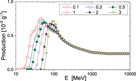
Figure 4.35. Energy dependence of proton production function for 26Al at different depths, as denoted in the legend in units of g cm−2, in the lunar sample 64455, calculated in Poluianov et al. (2018), reproduced with permission © ESO.
Download figure:
Standard image High-resolution imageDirect modeling (Poluianov et al. 2018) yields that for each depth below ∼5 g cm−2, there is an effective energy Eeff defined such that the production of 26Al at this depth is directly proportional (with a high accuracy) to the integral flux of protons with energy above Eeff for every reasonable spectral shape of SEP. This makes it possible to reconstruct, from the point-by-point measured depth profile of the isotope concentration in a lunar sample, the integral SEP spectrum, without any a priori assumptions on the spectral shape. Some examples of such reconstruction by Poluianov et al. (2018) are shown in Figure 4.36. Different colored symbols denote (as specified in the legend) SEP reconstructions based on different lunar samples and bounding assumptions on the not precisely known erosion rate. The full uncertainty range is shown as the gray-hatched stripe. One can see that the reconstruction is very robust for the energy range between 20 and 50 MeV, becoming less certain at higher energies and reaching a factor of ∼3 uncertainty at 80 MeV. We also note that most of earlier parametric estimates of the SEP spectrum from lunar samples agree with the direct reconstruction presented here, within the full range uncertainties of the latter (see details in Poluianov et al. 2018).

Figure 4.36. Integral omnidirectional fluxes
 of SEPs reconstructed (Poluianov et al.
2018, reproduced
with permission © ESO) for the past million of years based on 26Al
measured in lunar samples. The red and blue dots depict reconstructions for the
lunar samples 64455 and 74275, respectively. Open and solid symbols correspond to
different assumptions on the erosion rates, as denoted in the legend. The thick
line and the hatched area depict the average and full range of uncertainties of
the reconstructed fluxes for the two samples. The green stars with error bars
(variability between individual cycles) depict the mean values of
F30 and F60 for the last
solar cycles 1954–2008 (Reedy 2012).
of SEPs reconstructed (Poluianov et al.
2018, reproduced
with permission © ESO) for the past million of years based on 26Al
measured in lunar samples. The red and blue dots depict reconstructions for the
lunar samples 64455 and 74275, respectively. Open and solid symbols correspond to
different assumptions on the erosion rates, as denoted in the legend. The thick
line and the hatched area depict the average and full range of uncertainties of
the reconstructed fluxes for the two samples. The green stars with error bars
(variability between individual cycles) depict the mean values of
F30 and F60 for the last
solar cycles 1954–2008 (Reedy 2012).
Download figure:
Standard image High-resolution image
The mean SEP spectrum for the space era (Reedy 2012) is shown in Figure 4.36 as green stars with errors bars (representing the cycle-to-cycle variability). It is interesting to note that the SEP flux during the last solar cycles is totally consistent with the mean flux for the last million years (the green stars are within the gray-hatched area), even though the last 50 year period was characterized by enhanced solar activity (Solanki et al. 2004; Poluianov et al. 2018).
Of course, while lunar samples allow one to assess the spectra of SEP, the time resolution is lost completely, and no individual events can be identified. On the other hand, an integral probability density function (IPDF) can be evaluated within reasonable assumptions, such as the constancy of the IPDF on different timescales, from centennial to millions of years. This was done by Poluianov et al. (2018), who estimated for the Weibull distribution (Weibull 1951) and by combining different data sets (space-era data, cosmogenic isotopes in terrestrial archives, and in lunar samples) the IPDF of the SEP event occurrence on timescales from years to millions of years (Figure 2.16). One can see that different independent data sets, including lunar samples, are consistent with each other.
4.5.6. Other Data Sets
Unopened Lunar Samples
Some lunar core samples remain in sealed containers (Lofgren 2011; Shearer & Neal 2011). These have promise as excellent recorders of the lunar-volatile record that may have been partially lost in most lunar samples that have been exposed to the terrestrial atmosphere.
Lofgren (2011) noted that cores 69001, which appears to be of the top 27 cm of the lunar surface, and core 73001, which may be longer, would be of considerable interest. Recently, NASA began a new program (ANGSA) which may involve opening some of these sealed cores and other samples stored under vacuum or frozen.
Lunar Meteorites
Since 1982, at least 340 stones have been recovered and identified as ∼143 discrete meteorite falls recognized as having lunar composition. The total mass of 279 kg of documented meteorites, not counting a number of undocumented ones, is larger than the mass of rocks (not total material) recovered by the astronauts on the Moon (http://meteorites.wustl.edu/lunar/moon_meteorites_list_alumina.htm). The first documented lunar meteorite was Allan Hills 81005, which was recovered during an Antarctic expedition (Bogard & Johnson 1983). These are potential sources of SEP records if the material was removed close to the surface of the Moon, or was irradiated in space for a long-enough time. Most lunar meteorites are ejected from the Moon and land on Earth in a relatively short transit time (Eugster et al. 2006; Herzog & Caffee 2014). However, very few meteorites have SEP records as SEPs only affect the first few centimeters of the rock and in general, a few centimeters of the meteorite are ablated during entry into Earth's atmosphere. A number of lunar meteorites, however, show some effects. These include possible SEP 26Al in Calcalong Creek (Nishiizumi et al. 1992), QUE 93069 and 94269 (Nishiizumi et al. 1996). One lunar meteorite, Oued Alwitis 001, was shown in Wittmann et al. (2019) to have excess 14C and 26Al, which can only be explained due to SEP production. This sample appears to be saturated in both of these radionuclides.
Some Martian meteorites appear to contain SEP-produced nuclides including ALH 77005, LEW 88516, EET79001, Zagami, and Shergotty. Only a few other meteorites have been demonstrated to clearly have SEP effects (Salem, Evans et al. 1987; Nishiizumi et al. 1990), Madhipura and St. Severin (Michel et al. 1982), and Sutters Mill (Nishiizumi et al. 2014). In most cases, the ablation of the outer surface is a problem.
References
- Agostinelli S., Allison J. and Amako K. et al 2003 NIMPA 506 250
- Allison J., Amako K. and Apostolakis J. et al 2006 ITNS 53 270
- Allton J. H. and Waltz S. R. 1980 LPSC 11 1463
- Baker D. N., Li X. and Pulkkinen A. et al 2013 SpWea 11 585
- Bard E., Raisbeck G., Yiou F. and Jouzel J. 2000 TellB 52 985
- Bard E., Raisbeck G. M., Yiou F. and Jouzel J. 1997 E&PSL 150 453
- Baroni M., Bard E., Petit J.-R. and Viseur S. 2019 JGRD 124 7082
- Baroni M., Bard E., Petit J.-R., Magand O. and Bourlès D. 2011 GeCoA 75 7132
- Beer J. 2000 SSRv 93 107
- Beer J., Blinov A., Bonani G., Hofmann H. J. and Finkel R. C. 1990 Natur 347 164
- Beer J., Johnsen S. and Bonani G. 1992 in The Last Deglaciation: Absolute and Radiocarbon Chronologies Vol. 2 , ed E. Bard and W. S. Broecker et al (Berlin: Springer) 344
- Beer J., McCracken K. and von Steiger R. 2012 Cosmogenic Radionuclides Theory and Applications in the Terrestrial and Space Environments (Berlin: Springer)
- Begemann F., Born W., Palme H., Vilcsek E. and Wänke H. 1972 LPSC 3 1693
- Bentley H. W., Phillips F. M. and Davis S. N. et al 1982 Natur 300 737
- Berggren A.-M., Beer J. and Possnert G. et al 2009 GeoRL 36 L11801
- Binnie S. A., Nishiizumi K., Welten K. C., Caffee M. W. and Hoffmeister D. 2019 GeCoA 244 336
- Boeckl R. S. 1972 E&PSL 16 269
- Boenisch H., Engel A., Birner T., Hoor P., Tarasick D. W. and Ray E. A. 2011 ACP 11 3937
- Bogard D. D. and Hirsch W. C. 1975 LSPC 6 2057
- Bogard D. D. and Johnson P. 1983 Sci 221 651
- Bogard D. D., Nyquist L. E., Hirsch W. C. and Moore D. R. 1973 LSPC 4 79
- Böhlen T. T., Cerutti F. and Chin M. P. W. et al 2014 NDS 120 211
- Büntgen U., Wacker L. and Galván J. D. et al 2018 NatCo 9 5399
- Cliver E. W. and Dietrich W. F. 2013 JSWSC 3 A31
- Delaygue G., Bekki S. and Bard E. 2015 TellB 67 28582
- Delmas R. J., Beer J. and Synal H.-A. et al 2004 TellB 56B 492
- Desorgher L., Flückiger E. O., Gurtner M., Moser M. R. and Bütikofer R. 2005 IJMPA 20 6802
- Elmore D., Tubbs L. E. and Newman D. et al 1982 Natur 300 735
- Eugster O., Herzog G. F., Marti K. and Caffee M. W. 2006 Irradiation Records, Cosmic-Ray Exposure Ages, and Transfer Times of Meteorites (Tucson, AZ: Univ. of Arizona Press) 829
- Evans J. C., Fruchter J. S., Reeves J. H., Rancitelli L. A. and Perkins R. W. 1980 LPSC 11 1497
- Evans J. C., Reeves J. H. and Reedy R. C. 1987 LPSC 18 271
- Ferrari A., Sala P. R., Fasso A. and Ranft J. 2005 FLUKA: A Multi-particle Transport Code (Program Version 2005), CERN Yellow Reports: Monographs, CERN, Geneva, CERN-2005-010; INFN-TC-2005-11; SLAC-R-773
- Field C. V., Schmidt G. A., Koch D. and Salyk C. 2006 JGR 111 D15107
- Fink D., Klein J. and Middleton R. et al 1998 GeCoA 62 2389
- Finkel R. C., Arnold J. R. and Imamura M. et al 1971 LPSC 2 1773
- Fireman E. L. 1978 LPSC 2 1647
- Fireman E. L., D'Amico J. and Defelice J. 1973 LPSC 4 248
- Fireman E. L., D'Amico J. C. and Defelice J. C. 1970 Sci 167 566
- Fireman E. L., Defelice J. and Damico J. 1977 LPSC 8 3749
- Fruchter J. S., Rancitelli L. A. and Perkins R. W. 1976 LPSC 7 27
- Fruchter J. S., Reeves J. H., Evans J. C. and Perkins R. W. 1982 LPSC 12 567
- Geiss J., Eberhardt P., Bühler F., Meister J. and Signer P. 1970 JGR 75 5972
- Grinsted A., Moore J. C. and Jevrejeva S. 2007 PNAS 104 19730
- Güttler D., Adolphi F. and Beer J. et al 2015 E&PSL 411 290
- Hambaryan V. V. and Neuhäuser R. 2013 MNRAS 430 32
- Heck D., Knapp J., Capdevielle J. N., Schatz G. and Thouw T. 1998 CORSIKA: a Monte Carlo Code to Simulate Extensive Air Showers (Karlsruhe: Forschungszentrum Karlsruhe)
- Heiken G. H., Vaniman D. T. and French B. M. 1991 Lunar Sourcebook—A User's Guide to the Moon (Cambridge: Cambridge Univ. Press)
- Heikkilä U. 2007 PhD thesis
- Heikkilä U., Beer J. and Feichter J. 2008 ACP 8 2797
- Heikkilä U., Beer J. and Feichter J. 2009 ACP 9 515
- Heikkilä U., Beer J. and Feichter J. et al 2009 ACP 9 4145
- Heikkilä U., Phipps S. J. and Smith A. M. 2013 CliPa 9 2641
- Herzog G. F. and Caffee M. W. 2014 Cosmic-Ray Exposure Ages of Meteorites (Amsterdam: Elsevier) 419
- Hill-Falkenthal J., Priyadarshi A., Savarino J. and Thiemens M. 2013 JGRD 118 9444
- Hogg A. G., Hua Q. and Blackwell P. G. et al 2013 Radiocarbon 55 1889
- Holton J. R. 2004 An Introduction to Dynamic Meteorology Int. Geophysics Series 4th edn (Burlington, MA: Elsevier)
- Holton J. R., Haynes P. H. and McIntyre M. E. et al 1995 RvGeo 33 403
- Hua Q. and Barbetti M. 2014 Radiocarbon 46 1273
- Jacob D. J. and Prather M. J. 1990 TellB 42 118
- Jull A. J. T., Lal D. and Donahue D. J. 1995 E&PSL 136 693
- Jull A. J. T., Lal D., McHargue L. R., Burr G. S. and Donahue D. J. 2000 NIMPB 172 867
- Jull A. J. T., McHargue L. R. and Klandrud S. E. 2001 LPSC 32 1459
- Jull A. J. T., Panyushkina I. P. and Lange T. E. et al 2014 GeoRL 41 3004
- Jull A. J. T., Wilson G. C., Long J. V. P., Reed S. J. B. and Pillinger C. T. 1980 NucIM 168
- Jull A. J. T., Cloudt S. and Donahue D. J. et al 1998 GeCoA 62 3025
- Junge C. E. 1963 Air Chemistry and Radioactivity (International Geophysics Series) (New York: Academic)
- Kang J., Kim Y. and Son J. B. et al 2013 JKPS 63 1228
- Kerkweg A., Buchholz J. and Ganzeveld L. et al 2006 ACP 6 4617
- Khan T. R. and Perlinger J. A. 2017 GMD 10 3861
- Killen R. M. and Ip W.-H. 1999 RvGeo 37 361
- Kitts B. K., Podosek F. A. and Nichols R. H. et al 2003 GeCoA 67 4881
- Klein J., Fink D. and Middleton R. et al 1990 LPSC 21 635
- Koch D. M., Jacob D. J. and Graustein W. C. 1996 JGR 101 18651
- Kohl C. P., Murrell M. T., Russ G. P. and Arnold J. R. 1978 LPSC 9 2299
- Koldobskiy S. A., Kovaltsov G. A. and Usoskin I. G. 2018 SoPh 293 110
- Kovaltsov G. A. and Usoskin I. G. 2010 E&PSL 291 182
- Kovaltsov G. A., Mishev A. and Usoskin I. G. 2012 E&PSL 337 114
- Kravitz B., Robock A., Oman L., Stenchikov G. and Marquardt A. B. 2009 JGR 114
- Lal D., Jull A. J. T. and McHargue L. R. et al 2007 M&PSA 42 5086
- Lal D. and Peters B. 1962 in Progress in Elementary Particle and Cosmic Ray Physics Vol. 6 , ed J. G. Wilson and S. A. Wouthuysen (Amsterdam: North Holland) 77
- Lal D. and Peters B. 1967 Cosmic Ray Produced Radioactivity on the Earth (Berlin: Springer) 551
- Lanzerotti L. J., Reedy R. C. and Arnold J. R. 1973 Sci 179 1232
- Leppänen A.-P., Usoskin I. G., Kovaltsov G. A. and Paatero J. 2012 JASTP 74 164
- Li F., Austin J. and Wilson J. 2008 JCli 21 40
- Liang Q., Douglass A. R., Duncan B. N., Stolarski R. S. and Witte J. C. 2009 ACP 9 3011
- Lingenfelter R. E. 1963 RvGSP 1 35
- Lofgren G. E. 2011 (Houston, TX: Lunar and Planetary Institute) 36
- Lohmann U., Lüönd F. and Mahrt F. 2016 An Introduction to Clouds: From the Microscale to Climate (Cambridge: Cambridge Univ. Press)
- Marshall L., Schmidt A. and Toohey M. et al 2018 ACP 18 2307
- Masarik J. and Beer J. 1999 JGR 104 12099
- Masarik J. and Beer J. 2009 JGR 114 D11103
- Matthiä D., Herbst K., Heber B., Berger T. and Reitz G. 2013 SSRv 176 333
- Mekhaldi F., Muscheler R. and Adolphi F. et al 2015 NatCo 6 8611
- Menjo H., Miyahara H. and Kuwana K. et al 2005 ICRC (Pune) 2 357
- Meyer C. 2007a Lunar Sample Compendium: 15001-15006 Deep Drill Core, http://curator.jsc.nasa.gov/lunar/lsc/A15drill.pdf
- Meyer C. 2007b Lunar Sample Compendium: 60007-60001 Deep Drill Core, https://curator.jsc.nasa.gov/lunar/lsc/A16drill.pdf
- Meyer C. 2007c Lunar Sample Compendium: 70001-70006 Deep Drill Core, https://curator.jsc.nasa.gov/lunar/lsc/A17drill.pdf
- Meyer C. 2007d Lunar Sample Compendium: Summary of Apollo Drive Tubes, Revised, https://curator.jsc.nasa.gov/lunar/lsc/drive_tubes.pdf
- Meyer C. 2009 Lunar Sample Compendium: Introduction, https://curator.jsc.nasa.gov/lunar/lsc/intro.pdf
- Meyer H. O. A. and McCallister R. H. 1977 LPSC 8 664
- Meyer P., Parker E. N. and Simpson J. A. 1956 PhRv 104 768
- Michel R., Brinkmann G. and Stuck R. 1982 E&PSL 59 33
- Michel R., Leya I. and Borges L. 1996 NIMPB 113 434
- Mishev A. L., Usoskin I. G. and Kovaltsov G. A. 2013 JGRA 118 2783
- Miyake F., Horiuchi K. and Motizuki Y. et al 2019 GeoRL 46 11
- Miyake F., Masuda K. and Nakamura T. 2013 NatCo 4 1748
- Miyake F., Nagaya K., Masuda K. and Nakamura T. 2012 Natur 486 240
- Miyake F., Suzuki A. and Masuda K. et al 2015 GeoRL 42 84
- Muscheler R., Adolphi F., Herbst K. and Nilsson A. 2016 SoPh 291 3025
- Nishiizumi K., Arnold J. R. and Elmore D. et al 1979 E&PSL 45 285
- Nishiizumi K., Arnold J. R., Klein J. and Middleton R. 1984 E&PSL 70 164
- Nishiizumi K., Arnold J. R. and Kohl C. P. et al 2009 GeCoA 73 2163
- Nishiizumi K., Arnold R. J., Caffee W. M., Finkel C. R. and Reedy C. R. 1992 Antarctic Meteorites XVII Vol. 17 , ed E. M. Zolensky, M. Prinz and M. Lipschutz129
- Nishiizumi K. and Caffee M. W. 2001 Sci 294 352
- Nishiizumi K., Caffee M. W., Hamajima Y., Reedy R. C. and Welten K. C. 2014 M&PS 49 2056
- Nishiizumi K., Caffee M. W., Jull A. J. T. and Reedy R. C. 1996 M&PS 31 893
- Nishiizumi K., Caffee M. W. and Arnold J. R. 1998 in Lunar and Planetary Science XXVIII (Houston, TX: Lunar and Planetary Institute) 1027
- Nishiizumi K., Elmore D., Ma X. Z. and Arnold J. R. 1984 E&PSL 70 157
- Nishiizumi K., Fink D. and Klein J. et al 1997 E&PSL 148 545
- Nishiizumi K., Imamura M. and Kohl C. P. et al 1988 LPSC 18 79
- Nishiizumi K., Kubik P. W., Elmore D., Reedy R. C. and Arnold J. R. 1989 LPSC 19 305
- Nishiizumi K., Murrell M. T. and Arnold J. R. 1983 LPSC 14 B211
- Nishiizumi K., Nagai H. and Imamura M. et al 1990 Metic 25 392
- Obrien K. 1979 JGR 84 423
- O'Hare P., Mekhaldi F. and Adolphi F. et al 2019 PNAS 116 5961
- Park J., Southon J., Fahrni S., Creasman P. P. and Mewaldt R. 2017 Radiocarbon 59 1147
- Pavlov A. K., Blinov A. V. and Frolov D. A. et al 2017 JASTP 164 308
- Pavlov A. K., Blinov A. V. and Konstantinov A. N. et al 2013a MNRAS 435 2878
- Pavlov A. K., Blinov A. V. and Vasil'ev G. I. et al 2014 AstL 40 640
- Pavlov A. K., Blinov A. V. and Vasilyev G. I. et al 2013b AstL 39 571
- Pedro J., Van Ommen T. D. and Curran M. A. J. et al 2006 JGR 111 D21105
- Pedro J. B., Smith A. M. and Duldig M. L. et al 2009 in Advances in Geosciences, Vol. 14, Solar Terrestrial (ST), 10Be Concentrations in Snow at Law Dome, Antarctica Following the 29 October 2003 and 20 January 2005 Solar Cosmic Ray Events (Singapore: World Scientific) 285
- Pedro J. B., Smith A. M., Simon K. J., van Ommen T. D. and Curran M. A. J. 2011 CliPa 7 707
- Pepin R. O., Basford J. R., Dragon J. C., Coscio M. R. and Murthy V. R. 1974 LPSC 5 2149
- Pierce J. R., Weisenstein D. K., Heckendorn P., Peter T. and Keith D. W. 2010 GeoRL 37 L18805
- Pinto J. P., Turco R. P. and Toon O. B. 1989 JGR 94 11165
- Plumb R. A. 2002 JMSJ 80 793
- Poluianov S., Kovaltsov G. A. and Usoskin I. G. 2018 A&A 618 A96
- Poluianov S. V., Kovaltsov G. A., Mishev A. L. and Usoskin I. G. 2016 JGRD 121 8125
- Proedrou E. and Hocke K. 2016 EP&S 68 96
- Raisbeck G. M., Yiou F. and Fruneau M. et al 1981 Natur 292 825
- Rao M. N., Garrison D. H., Bogard D. D. and Reedy R. C. 1994 GeCoA 58 4231
- Rasmussen S. O., Andersen K. K. and Svensson A. M. et al 2006 JGR 111 D06102
- Raukunen O., Vainio R. and Tylka A. J. et al 2018 JSWSC 8 A04
- Reedy R. 1998 PIASE 107 433
- Reedy R. C. 1977 TANS 27 198
- Reedy R. C. 1980 in The Ancient Sun: Fossil Record in the Earth, Moon and Meteorites , ed R. O. Pepin, J. A. Eddy and R. B. Merrill (Houston, TX: Lunar and Planetary Institute) 365
- Reedy R. C. 2012 LPSC 43 1285
- Reedy R. C., Arnold J. R. and Lal D. 1983 Sci 219 127
- Reedy R. C. and Marti K. 1991 in The Sun in Time , ed C. P. Sonett, M. S. Giampapa and M. S. Matthews (Tucson, AZ: Univ. of Arizona Press) 260
- Reedy R. C. and Nishiizumi K. 1998 LPSC 29 1698
- Roth R. and Joos F. 2013 CliPa 9 1879
- Röthlisberger R., Mulvaney R. and Wolff E. W. et al 2003 JGRD 108 4526
- Russ G. P., Burnett D. S. and Wasserburg G. J. 1972 E&PSL 15 172
- Russ G. P. and Emerson M. T. 1980 The Ancient Sun: Fossil Record in the Earth, Moon and Meteorites , ed R. O. Pepin, J. A. Eddy and R. B. Merrill (Oxford: Pergamon) 387
- Ryder G. and Norman M. D. 1980 Catalog of Apollo 16 Rocks: Part II, Technical Report, NASA JSC
- Seinfeld J. H. and Pandis S. N. 2006 Atmospheric Chemistry and Physics: From Air Pollution to Climate Change (New York: Wiley)
- Shearer C. K. and Neal C. R. 2011 in LPI Contribution, Vol. 1621, A Wet Vs. Dry Moon: Exploring Volatile Reservoirs and Implications for the Evolution of the Moon and Future Exploration (Houston, TX: Lunar and Planetary Institute) 56
- Shedlovsky J. P., Honda M. and Reedy R. C. et al 1970 GeCAS 1 1503
- Sheng J.-X., Weisenstein D. K. and Luo B.-P. et al 2015 JGRD 120 256
- Sigl M., Winstrup M. and McConnell J. R. et al 2015 Natur 523 543
- Simon K. J., Pedro J. B., Smith A. M., Child D. P. and Fink D. 2013 NIMPB 294 208
- Simpson J. A. 1960 JGR 65 1615
- Sisterson J. M., Schneider R. J. and Beverding A. et al 1996 LPSC 27 1207
- Škerlak B., Sprenger M. and Wernli H. 2014 ACP 14 913
- Solanki S. K., Usoskin I. G., Kromer B., Schüssler M. and Beer J. 2004 Natur 431 1084
- Stoenner R. W., Lyman W. J. and Davis R. 1970 GeCAS 1 1583
- Stohl A. 2006 JGR 111 D11306
- Sukhodolov T., Usoskin I. G. and Rozanov E. et al 2017 NatSR 7 45257
- Synal H.-A., Beer J. and Bonani G. et al 1990 NIMPB 52 483
- Talpos S. and Cuculeanu V. 1997 J. Environ. Radioact. 36 93
- Timmreck C. 2012 ClCh 3 545
- Tost H., Jöckel P. and Kerkweg A. et al 2007 ACP 7 2733
- Tost H., Jöckel P., Kerkweg A., Sander R. and Lelieveld J. 2006 ACP 6 565
- Tost H., Lawrence M. G. and Bruehl C. et al 2010 ACP 10 1931
- Usoskin I. G. and Kovaltsov G. A. 2008 JGR 113 D12107
- Usoskin I. G. and Kovaltsov G. A. 2012 ApJ 757 92
- Usoskin I. G., Kromer B. and Ludlow F. et al 2013 A&A 552 L3
- Usoskin I. G., Solanki S. K., Kovaltsov G. A., Beer J. and Kromer B. 2006 GeoRL 33 L08107
- Uusitalo J. et al 2018 NatCo 9 3495
- Veeder C. 2009 PhD thesis
- Vet R., Artz R. S. and Carou S. et al 2014 AtmEn 93 3
- Visioni D., Pitari G., Tuccella P. and Curci G. 2018 ACP 18 2787
- Wagnon P., Delmas R. J. and Legrand M. 1999 JGR 104 3423
- Wahlen M., Honda M. and Imamura M. et al 1972 LPSC 3 1719
- Webber W. R., Higbie P. R. and McCracken K. G. 2007 JGRA 112 A10106
- Webber W. R. and Higbie P. R. 2003 JGR 108 1355
- Weibull W. 1951 JAM 18 293
- Weisenstein D. K., Keith D. W. and Dykema J. A. 2015 ACP 15 11835
- Werner J. et al 2017 Los Alamos National Laboratory, LA-UR-17-29981
- Wieler R. 1998 SSRv 85 303
- Wieler R., Baur H. and Signer P. 1986 GeCoA 50 1997
- Wieler R. and Heber V. S. 2003 SSRv 106 197
- Winglee R. M. and Harnett E. M. 2007 GeoRL 34 L21103
- Winkler R., Landais A. and Risi C. et al 2013 PNAS 110 17674
- Wittmann A., Korotev R. L. and Jolliff B. L. et al 2019 M&PS 54 2167
- Wurz P., Rohner U. and Whitby J. A. et al 2007 Icar 191 486
- Yaniv A. and Marti K. 1981 ApJ 247 L143
- Zerle L., Faestermann T. and Knie K. et al 1997 JGRD 102 19517
- Zhou T., Geller M. A. and Hamilton K. 2006 JAtS 63 2740