
Abstract
Predicting the output of quantum circuits is a hard computational task that plays a pivotal role in the development of universal quantum computers. Here we investigate the supervised learning of output expectation values of random quantum circuits. Deep convolutional neural networks (CNNs) are trained to predict single-qubit and two-qubit expectation values using databases of classically simulated circuits. These circuits are built using either a universal gate set or a continuous set of rotations plus an entangling gate, and they are represented via properly designed encodings of these gates. The prediction accuracy for previously unseen circuits is analyzed, also making comparisons with small-scale quantum computers available from the free IBM Quantum program. The CNNs often outperform these quantum devices, depending on the circuit depth, on the network depth, and on the training set size. Notably, our CNNs are designed to be scalable. This allows us exploiting transfer learning and performing extrapolations to circuits larger than those included in the training set. These CNNs also demonstrate remarkable resilience against noise, namely, they remain accurate even when trained on (simulated) expectation values averaged over very few measurements.
Export citation and abstract BibTeX RIS

Original content from this work may be used under the terms of the Creative Commons Attribution 4.0 license. Any further distribution of this work must maintain attribution to the author(s) and the title of the work, journal citation and DOI.
1. Introduction
Universal quantum computers promise to solve some relevant computational problems which are intractable for classical computers [1, 2]. In fact, the claim of quantum speed-up is justified only when the targeted computational task cannot be completed by any classical algorithm in a comparable computation time [3]. On the other hand, precisely the lack of efficient classical simulation methods hinders the further engineering of quantum devices with more and more qubits, as their development has to proceed without benchmark data. In this context, machine-learning techniques represent an attractive alternative to direct classical simulations, since they might feature a lower computational cost. In fact, supervised machine learning from classically simulated datasets has already emerged as a promising and computationally feasible strategy to predict the ground-state properties of complex quantum systems, including, e.g. small molecules [4, 5], solid-state systems [6, 7], atomic gases [8, 9], and protein-ligand complexes [10, 11]. Moreover, it has recently been proven that data-based algorithms can solve otherwise classically intractable computational tasks [12], including predicting ground-state properties of quantum systems, and rigorous guarantees on the accuracy and on the scaling of the required training set size have been demonstrated [13]. Still, producing training sets for supervised learning via classical computers quickly becomes unfeasible as the system size increases. In the context of ground-state simulations, this problem has been addressed via scalable neural networks [14, 15]. These allow performing transfer learning from small to large systems [9, 16], and even to extrapolate to sizes larger than those included in the training set. So, it is natural to wonder whether neural networks might also be trained to emulate quantum circuits, and whether they might extrapolate to large qubit numbers where exact simulation methods become problematic.
The above considerations led us to investigate the supervised learning of gate-based quantum computers. Our goal is to demonstrate that deep convolutional neural networks (CNNs) can be trained to predict relevant output properties of quantum circuits, both from exact classical simulations of expectation values, as well as from noisy (simulated) measurements. Remarkably, we show that the CNNs trained on random circuits are able to emulate a broad category of quantum circuits, including, e.g. the Bernstein–Vazirani (BV) algorithm. Furthermore, thanks to a properly designed scalable structure, they provide accurate extrapolations for circuits larger than those included in the training set. Our findings also support the long-term perspective of using quantum computers to produce training data for supervised learning, possibly allowing them to emulate classically intractable algorithms. Clearly, if distributed to many users, such trained networks would allow these users to benefit from the quantum device even without having direct access to it.
In detail, in this article we consider large ensembles on quantum circuits built with gates randomly selected (mostly) from a discrete approximate universal set. It is worth mentioning that the sampling from random circuits is the computational task considered in the recent demonstrations of quantum supremacy [17, 18]. A second gate set, including continuous rotations plus an entangling layer, is addressed in the  and circuit depths (number of gates per qubit) up to
  . Significantly larger circuits are also considered in the testing processes performed via extrapolation procedures. Deep CNNs are trained to map the circuit descriptors to the output expectation values. The CNNs are tested on previously unseen circuits, and we analyze how the predictions accuracy varies as a function of the circuit size, of the network depth, and of the training-set size. We also compare the accuracy of the trained CNNs against the one of various small quantum computers available via IBM Quantum Experience [21]. Generally, the CNNs outperform the freely available noisy intermediate-scale quantum (NISQ) processors, unless the circuit's depth is increased at fixed CNN parameters. Notably, our CNNs are designed to be scalable. This allows us investigating transfer-learning and extrapolation protocols. Specifically, we show that the learning of large circuits can be accelerated via a pretraining performed on smaller circuits. Furthermore, we employ CNNs trained on small circuits to predict the output of circuits with more qubits, up to twice as much (or even more for continuous circuits). Interestingly, CNNs also learn (from random circuits) to emulate the BV algorithm, even when the number of qubits is increased by several orders of magnitude. Finally, we consider the training on noisy expectation values, obtained as averages over a variable number of (simulated) measurements. We find that the CNNs are able to filter this noise, providing remarkably accurate estimates of the exact expectation values even when very few measurements are considered in the training data. This validates the idea of using data produced by NISQ computers to train deep neural networks.
The rest of the article is organized as follows: in section 2 we describe the random circuits built using the discrete approximate universal sets, the appropriate one-hot encoding we design for supervised learning, the CNNs we adopt, and the target expectation values. Furthermore, we discuss the class of random circuits that can be emulated from the target values we address. The predictions of the trained CNNs are analyzed in section 3. In the same section these predictions are also compared with those obtained with small quantum computers available from IBM Quantum Experience. Then, transfer learning and extrapolation protocols are analyzed; notably, in the same section we also discuss the training on noisy expectation values. Section 4 reports our conclusions and an outlook on future perspectives. In the
2. Methods
2.1. Representation of random circuits
Our goal is to train deep CNNs to map univocal representations of random circuits to their output expectation values. Specifically, we mostly consider circuits built with two single-qubit gates, namely, the T-gate (T) and the Hadamard gate (H), together with one two-qubit gate, namely, the controlled-not gate (CX). Notably, the set  constitutes an approximately universal set [22, 23], meaning that any unitary operator can be implemented using these three gates. It is worth noticing that the identity
  can be represented as
  . Below, an extended set explicitly including the gate I will be discussed. We adopt the standard computational basis corresponding to the eigenstates of the Pauli matrix
  . In this basis, the three considered gates are represented by the following matrices:

In the following, we consider circuits with N qubits and P layers of gates. Therefore, the integer P corresponds to the number of gates per qubit; this parameter will be referred to also as the circuit depth. In every layer, each qubit is processed by a gate randomly selected from the set  . Notice that the two-qubit gate CX acts on a control and on a target qubit. To simplify the circuit representation, we allow only one CX gate at every layer. Circuits with more CX gates per layer can be emulated by deeper circuits satisfying the constraint. This constraint allows us adopting a relatively simple univocal circuit representation. It is based on the following one-hot encoding of the gate acting on each qubit: the T-gate corresponds to the vector
  , the H-gate to
  , the control qubit of the CX-gate corresponds to
  , while the target qubit corresponds to
  . This map is also represented in figure 1. Therefore, the feature vector representing a random circuit is a four-channel two-dimensional binary matrix with dimensions
  . Analogous gate-based descriptions of quantum circuits have been adopted in [24, 25]. Despite the constraint on the number of CX gates per layer, the number Q of possible circuits rapidly grows with N and P. This number can be computed as:

where m is the number of CX-gates in the circuit. The first term, namely,  , represents the possible combinations considering only the T-gates and the H-gates. The second term, namely,
  , corresponds to the possible combinations of the CX-gates in P layers. The third term, namely, 2m
, corresponds to the choice of the control and of the target qubit for each CX gate. Finally, the term
, corresponds to the possible combinations of the CX-gates in P layers. The third term, namely, 2m
, corresponds to the choice of the control and of the target qubit for each CX gate. Finally, the term  corresponds to the available pairs for each CX-gate. For example, for the smallest circuit size considered in this article, namely, N = 3 and P = 5, one has
  possible random circuits. For the largest size, namely, N = 20 and P = 6, one has the astronomic number
  . This means that it is virtually impossible to create a dataset exhausting the whole ensemble of possible circuits. We instead resort to the generalization capability of deep CNNs. These are expected to provide accurate predictions for previously unseen instances, even when trained on (largely non-exhaustive) training sets including a number
  of training instances.

Figure 1. Visualization of the one-hot encoding that represents the quantum gates in the set  . The full circle and the empty circle with plus sign represent the control and the target qubit of the CX gate, respectively.
Download figure:
Standard image High-resolution imageWhile the set  is, in principle, universal, the choice of operating on all qubits in every layer implies that some unitary operators cannot be represented. Therefore, we also consider the extended set
  , where the identity is explicitly included. For this set, a five channel one-hot encoding is needed. We use the map represented in figure 2. Most of the results reported in this article are based on the set
  , unless stated otherwise. Notably, this set is flexible enough to represent the BV algorithm, which we use as a relevant test bed. For a few representative test cases, we also consider the extended gate set
  , finding very similar performances. Furthermore, an additional gate set is addressed in the
  and
and  , which lead to discrete values of the outputs. Also, in this continuous set the number of entangling gates scales with N, thus possibly representing a more stringent test for the extrapolation procedure.

Figure 2. Visualization of the one-hot encoding that represents the quantum gates in the set  .
.
Download figure:
Standard image High-resolution image2.2. Target values
The output state of a quantum circuit can be written as

where the tensor product  is the input state and the unitary operator U represents the sequence of quantum gates that constitute the circuit. Here and in the following, we indicate with
  and
and  the eigenvectors of the Pauli operator Zi
acting on qubit
the eigenvectors of the Pauli operator Zi
acting on qubit  , such that
  and
and  . With this notation, each state
  of the many-qubit computational basis corresponds to a bit string
  , where
  for
for  . Our goal is to perform supervised learning of output expectation values. First, we focus on the single-qubit expectation values

These expectation values can be computed as

It is convenient to perform the following rescaling:

so that ![$z_i\in[0,1]$](https://content.cld.iop.org/journals/2058-9565/8/2/025022/revision3/qstacc4e2ieqn37.gif) , and
, and  corresponds to
  , while
  corresponds to
  . The rescaled variable zi
is the first target value we address for supervised learning. It is worth anticipating that we will consider both CNNs designed to predict only one expectation value, say, z1, and CNNs that simultaneously predict all single-qubit expectation values zi
, for
. The rescaled variable zi
is the first target value we address for supervised learning. It is worth anticipating that we will consider both CNNs designed to predict only one expectation value, say, z1, and CNNs that simultaneously predict all single-qubit expectation values zi
, for  . This is discussed with more details in section 2.4.
For illustrative purposes, we show in figure 3 the distribution of the target value z1 over an ensemble of random circuits built with  . Four representative circuit sizes are considered. Clearly, here the possible expectation values are discrete. In particular, one notices a relatively large probability of the output value
  . Circuits with continuous outputs are considered in the

Figure 3. Normalized histograms of the rescaled single-qubit expectation values  over ensembles of random circuits. Different number of qubits N and circuit depths P are considered in the four panels: N = 3 and P = 5 (a); N = 3 and P = 20 (b); N = 5 and P = 10 (c); N = 20 and P = 6 (d). The ensembles in (a)–(c), and the one in (d) include 5000 and 2000 circuits, respectively.
Download figure:
Standard image High-resolution imageThe second target values we consider are the two-qubit expectation values  , where, in general,
  . Specifically, we focus on the case i = 1 and j = 2, and the target value is the rescaled variable:

Clearly, single-qubit and two-qubit Pauli-Z expectation values represent a limited description of the circuit output. However, this information is sufficient to unambiguously identify the output of a significant category of quantum circuits. This category is described in the following subsection, where we also discuss some relevant examples belonging to the category.
2.3. Emulable quantum algorithms
For certain quantum algorithms, only a small subset of the 2N
output bit strings have non-zero measurement probability. In fact, some relevant circuits have only one possible outcome (in the absence of noise and errors). These are discussed below. First, we consider the more generic category for which only two output bit strings, which we indicate as a and b, have non-zero measurement probabilities  and
and  . With this notation, one has
  . For this category of circuits, the expectation values
  and
and  provide all the information required to unambiguously identify the bit strings a and b. This statement is proven here by providing an explicit algorithm. It is assumed that
  for
for  and that the expectation values mentioned above are known. It is worth emphasizing that, in fact, if
  , knowledge of the single-qubit expectation values suffices. Indeed, the values
  are only used when
  —see case iv) below—and such case is easily identified since one must have
  for at least one qubit i.
Proof. The qubit are analyzed in the order  . Four possible cases have to be separately treated:
- (i)If
 , the corresponding bits are set to .
 - (ii)If, one sets .
- (iii)If and either i = 1 or i > 1 with for we arbitrarily set, without loss of generality, and . Notice that we can also infer the two probabilities: and .
- (iv)Otherwise, when (this is known from case iii)), two expectation values are possible. One is , where the integer is the first index such that (at least one exists); in this case one sets and . If, instead, , one sets and . When , one must have , and we also know that an integer such that exists. In this situation, . If , one sets and . If, instead, , one sets and .


![$j\in[1,i-1]$](https://content.cld.iop.org/journals/2058-9565/8/2/025022/revision3/qstacc4e2ieqn73.gif)


![$j\in[1,i-1]$](https://content.cld.iop.org/journals/2058-9565/8/2/025022/revision3/qstacc4e2ieqn82.gif)


As discussed in the previous paragraph, the single-qubit expectation values  , eventually combined with
  , are sufficient to identify the output bit strings when only two of them have non-zero probability. Clearly, the values
  are sufficient when only one bit string is possible. Interestingly, some paradigmatic quantum algorithm belong to this group. A relevant example is the Deutsch–Jozsa algorithm [26]. This allows assessing whether a Boolean function
  is either constant or balanced. The algorithm involves measuring the first N − 1 qubits. If the outcome corresponds to the bit string
  , the function is constant, otherwise the function is balanced. Predicting N − 1 single-qubit expectation values allows reaching the same result. Practically, if
  for
for  , the only possible bit string is the bit string
  , corresponding to a constant function. Otherwise, the function is balanced. Also in the BV algorithm [19] there is only one possible outcome. This algorithm is designed to identify an unknown bit string
  , assuming we are given an oracle that implements the Boolean function
  defined as
  , where the symbol
  represents the dot product modulo 2. Notably, the BV algorithm provides the answer with one function query, outperforming classical computers which require N − 1 queries. Single-qubit expectation values allow identifying w:
  corresponds to
  , while
  corresponds to
  . The Grover algorithm with two searched items [27] and the quantum counting algorithm [28] have two output bit strings with much higher probabilities than the other strings. Therefore one could use the predictions for
  and
and  to emulate also these latter algorithms.
2.4. CNNs and training protocol
The CNNs considered in this article have the overall architecture described in figure 4. Relevant variations occur mostly in the last layer. Therein, the number of neurons corresponds to the desired number of outputs No
. Specifically, we consider CNNs designed to predict only one expectation value at a time ( ), as well as N expectation values simultaneously (
 ). Clearly, in the first case, the last layer includes only one neuron. In the second case, it includes N neurons. The overall network structure we adopt is standard in fields such as, e.g. image classification or object detection. The first part includes Nc
multi-channel convolutional layers, which create filtered maps of their input. The maps are created by scanning the input using (typically small) filters, featuring a fixed number of parameters. It is worth pointing out that the size of a convolutional layer's output scales with the corresponding input, even though the number of parameters in the filter is fixed. In turn, this means that the same filters could be applied to different input sizes. As in standard CNNs, the output of the convolutional part of the network is connected to a few dense layers (four in our case) with all-to-all interlayer connectivity. These dense layers constitute the venue where high-level operations on the effective features extracted by the convolutional layers occur. In standard CNNs, the connection between the last convolutional layer and the first dense layer is commonly performed through so-called flatten layers. This choice forces to scale the width (i.e. the number of neurons and of the corresponding parameters) of the first dense layer with the size of the network's input. Therefore, the whole network would be applicable only to one circuit size. Instead, we perform the connection using a global pooling layer. This extracts the maximum values of each (whole) map in the last convolutional layer. Thus, the output size of the convolutional part gets fixed: it corresponds to the number of filters in the last convolutional layer. This feature was adopted in [15] for the supervised learning of ground-state energies of quantum systems. It allowed implementing scalable CNNs, i.e. networks that can be trained on heterogeneous datasets including different system sizes and that can predict properties for sizes larger than those included in the training set. Scalable networks for physical and chemical systems have been implemented also in [9, 14, 16, 29, 30], using different strategies. Here, we exploit the global pooling layer to allow a single CNN addressing different circuit sizes. Notice, however, that full scalability is obtained only when the CNN predicts only one expectation value (with a single neuron in the output layer) at a time. More expectation values corresponding to different qubits can, in fact, be predicted even by the single output network. However, these predictions have to be performed in a sequential manner, by feeding the network with an appropriate swapping of the features. Specifically, when the goal is to predict, say, zj
, for any
). Clearly, in the first case, the last layer includes only one neuron. In the second case, it includes N neurons. The overall network structure we adopt is standard in fields such as, e.g. image classification or object detection. The first part includes Nc
multi-channel convolutional layers, which create filtered maps of their input. The maps are created by scanning the input using (typically small) filters, featuring a fixed number of parameters. It is worth pointing out that the size of a convolutional layer's output scales with the corresponding input, even though the number of parameters in the filter is fixed. In turn, this means that the same filters could be applied to different input sizes. As in standard CNNs, the output of the convolutional part of the network is connected to a few dense layers (four in our case) with all-to-all interlayer connectivity. These dense layers constitute the venue where high-level operations on the effective features extracted by the convolutional layers occur. In standard CNNs, the connection between the last convolutional layer and the first dense layer is commonly performed through so-called flatten layers. This choice forces to scale the width (i.e. the number of neurons and of the corresponding parameters) of the first dense layer with the size of the network's input. Therefore, the whole network would be applicable only to one circuit size. Instead, we perform the connection using a global pooling layer. This extracts the maximum values of each (whole) map in the last convolutional layer. Thus, the output size of the convolutional part gets fixed: it corresponds to the number of filters in the last convolutional layer. This feature was adopted in [15] for the supervised learning of ground-state energies of quantum systems. It allowed implementing scalable CNNs, i.e. networks that can be trained on heterogeneous datasets including different system sizes and that can predict properties for sizes larger than those included in the training set. Scalable networks for physical and chemical systems have been implemented also in [9, 14, 16, 29, 30], using different strategies. Here, we exploit the global pooling layer to allow a single CNN addressing different circuit sizes. Notice, however, that full scalability is obtained only when the CNN predicts only one expectation value (with a single neuron in the output layer) at a time. More expectation values corresponding to different qubits can, in fact, be predicted even by the single output network. However, these predictions have to be performed in a sequential manner, by feeding the network with an appropriate swapping of the features. Specifically, when the goal is to predict, say, zj
, for any ![$j\in[2,N]$](https://content.cld.iop.org/journals/2058-9565/8/2/025022/revision3/qstacc4e2ieqn111.gif) , one can employ a CNN trained to predict z1, swapping the rows 1 and j of the network's input. If, instead, the goal is to simultaneously predict the expectation values corresponding to all qubits, obviously the number of neurons in the last layer has to be adapted to the targeted qubit number. In this case, full scalability is lost, since more parameters have to be trained if the qubit number increases.
, one can employ a CNN trained to predict z1, swapping the rows 1 and j of the network's input. If, instead, the goal is to simultaneously predict the expectation values corresponding to all qubits, obviously the number of neurons in the last layer has to be adapted to the targeted qubit number. In this case, full scalability is lost, since more parameters have to be trained if the qubit number increases.

Figure 4. Representation of the CNN for the illustrative case of N = 3 qubits and circuit depth P = 5. Boxes report the input and the output shapes of each layer. This example includes  convolutional layers (Conv2D). Their input and output shapes have dimensions: (B, L1, L2, F), where
  is the mini-batch size (not specified),
  and
and  denote the size of the two-dimensional feature maps, while F is the number of filters. For the dense layers (Dense), we only have the mini-batch size and the number of nodes. The figure omits the batch normalization layers, included in every layer before the application of the activation function. The latter corresponds to the Mish function [32], except for the last node where it corresponds to the sigmoid function. It is worth highlighting the global maximum pooling layer (GlobalMaxPooling2D) connecting the last convolutional layer to the first dense layer.
Download figure:
Standard image High-resolution imageThe training of the CNN is performed by minimizing the loss function. For the discrete circuits, we adopt the binary cross-entropy:

where  is the number of instances in the training set, No
is the number of outputs (corresponding to the number of nodes in the last dense layer), and
is the number of instances in the training set, No
is the number of outputs (corresponding to the number of nodes in the last dense layer), and  is the network prediction corresponding to the ground-truth target value
  . As discussed above, we consider the cases
  and
and  . In the first case, the N target values correspond to all rescaled single-qubit expectation values:
  , for
, for  . In the latter case, we consider only one (rescaled) single-qubit expectation value, namely,
  , or one (rescaled) two-qubit expectation value, namely,
  . The optimization method we adopt is a successful variant of the stochastic gradient-descent algorithm, named Adam [31]. No benefit is found by introducing a regularization term in the loss function. Instead, batch normalization layers are included after every layer, before the application of the activation function. The chosen mini-batch size is in the range
 ![$N_b\in [128,512]$](https://content.cld.iop.org/journals/2058-9565/8/2/025022/revision3/qstacc4e2ieqn121.gif) , depending on the training set size. The CNNs are trained on large ensembles of random quantum circuits. These are implemented and simulated using the Qiskit library. These simulations provide numerically exact predictions for the considered expectation values. We also consider noisy estimates of the expectation values obtained from finite samples of simulated measurements. These estimates are employed in section 3.3 to inspect the impact of errors in the training set on the prediction accuracy. After training, the CNNs are tested on previously unseen random circuits. It is also worth mentioning that we remove possible circuit replicas, both in the training and in the test sets. In fact, only for the smallest circuits we consider, corresponding to N = 3 and P = 5, one can find within
, depending on the training set size. The CNNs are trained on large ensembles of random quantum circuits. These are implemented and simulated using the Qiskit library. These simulations provide numerically exact predictions for the considered expectation values. We also consider noisy estimates of the expectation values obtained from finite samples of simulated measurements. These estimates are employed in section 3.3 to inspect the impact of errors in the training set on the prediction accuracy. After training, the CNNs are tested on previously unseen random circuits. It is also worth mentioning that we remove possible circuit replicas, both in the training and in the test sets. In fact, only for the smallest circuits we consider, corresponding to N = 3 and P = 5, one can find within  training circuits a non-negligible number of identical replicas.
3. Results
3.1. Single-qubit expectation values
The CNNs described in section 2.4 are trained to map the circuit descriptors (see section 2.1) to various outputs. We first focus on a CNN designed to simultaneously predict the rescaled single-qubit expectation values zi
, with  . Here, the discrete gate sets are considered. Figure 5 displays the scatter plots of predicted versus ground-truth expectation values, for four representative circuit sizes. The tests are performed on random circuits distinct from those included in the training set. One notices a close correspondence in all four examples. In figure 6, we analyze how the prediction accuracy varies with the circuit depth P. Three datasets correspond to random circuits generated with the gates from the discrete set
  , but with different qubit numbers N. For the fourth dataset the gates are sampled from the extended set
  (see section 2.1). To quantify the accuracy, we consider the coefficient of determination:

where  is the prediction associated to the ground-truth target value
  ,
,  is the average of the target values,
  is the number of random circuits in the test set, and No
is the number of outputs. In this case, we have
is the number of random circuits in the test set, and No
is the number of outputs. In this case, we have  outputs. It is worth stressing that R2 quantifies the accuracy in relation to the intrinsic variance of the test data. Indeed, it accounts for the (mean squared) deviations from the ground-truth values, compared to the typical fluctuations from the mean. This metric is therefore suitable for fair comparisons among different circuits sizes, which might display a more or less pronounced tendency of the output values to cluster at or close a mean value. For small P one observes remarkably high scores
  , corresponding to essentially exact predictions. However, the accuracy significantly decreases for deeper circuits. It is worth pointing out that, in this analysis, the depth of the CNN is not varied, and the training set size is also fixed at
  .
.

Figure 5. Rescaled single-qubit expectation values  predicted by the CNN versus the ground-truth results
  , with
  . The latter results are simulated via Qiskit. Different number of qubits N and circuit depths P are considered in the four panels: N = 3 and P = 5 (a); N = 3 and P = 7 (b); N = 5 and P = 5 (c); N = 5 and P = 7 (d). These test sets include 100 random circuits. The color scale (blue to yellow) represents the absolute discrepancy
  . The (red) line represents the bisector
  .
.
Download figure:
Standard image High-resolution image
Figure 6. Coefficient of determination R2 for rescaled single-qubit expectation values zi
as a function of the circuits depth P. Three datasets correspond to random circuits built with gates from the set  , but having different qubit numbers N (see legend). For the fourth dataset, the extended gate set
  is used. For P = 5 the neural network is trained from scratch on
  instances, while for P > 5 the training starts with the optimized weights and biases for P − 1.
Download figure:
Standard image High-resolution imageThe prediction accuracy can be improved by enlarging the training set, or by increasing the depth of the CNN. The first approach is analyzed in figure 7, for three representative circuit sizes. One notices the typical power-law suppression (see, e.g. [4, 33]) of the prediction error  , where α > 0 is a non-universal exponent. The second approach is analyzed in figure 8. We find that the R2 score systematically increases with the number of convolutional layers Nc
. It is worth pointing out that the deepest CNNs adopted in this article include around
, where α > 0 is a non-universal exponent. The second approach is analyzed in figure 8. We find that the R2 score systematically increases with the number of convolutional layers Nc
. It is worth pointing out that the deepest CNNs adopted in this article include around  parameters. This number does not represent a noteworthy computational burden for modern high-performance computers, in particular if equipped with state-of-the-art graphic processing units. In fact, significantly deeper neural networks are routinely trained in the field of computer vision. Relevant examples are VGG-16, VGG-19 [34] and ConvNeXt [35]. Instead, creating copious training sets for circuits with N > 10 qubits becomes computationally expensive. In fact, simulating circuits with
  qubits is virtually impossible, unless the analysis is restricted to specific circuits types for which tailored algorithms exist. Relevant examples are slightly entangling circuits and those dominated by Clifford gates; these two circuit types can be efficiently simulated via tensor-network methods and near-Clifford algorithms [36], respectively. Two strategies to circumvent the computational-cost problem are discussed in the section 3.2. With the second, predictions for large qubit numbers can be provided, without additional computational burdens in the training process, even in the regime where exact circuit simulations via general-purpose algorithms become impractical.

Figure 7. Normalized prediction error  for (rescaled) single-qubit expectation values zi
as a function of the training set size
for (rescaled) single-qubit expectation values zi
as a function of the training set size  . Three datasets correspond to random circuits built with gates from the set
  , but having different qubit numbers N and circuit depths P (see legend). For the fourth dataset, the extended gate set
  is used. The adopted CNN is described in figure 4.
Download figure:
Standard image High-resolution image
Figure 8. Coefficient of determination R2 for rescaled single-qubit expectation values zi
as a function of the number of convolutional layers Nc
. The qubit number is N = 3 and the circuit depth is P = 7. The training set includes  random circuits. The employed CNN is similar to the one depicted in figure 4, but with two fully-connected layers including 100 and 50 neurons. The Nc
convolutional layers include F = 32 filters. The batch normalization layers and the output layer act as described in figure 4.
random circuits. The employed CNN is similar to the one depicted in figure 4, but with two fully-connected layers including 100 and 50 neurons. The Nc
convolutional layers include F = 32 filters. The batch normalization layers and the output layer act as described in figure 4.
Download figure:
Standard image High-resolution image3.2. Transfer learning and extrapolation
We exploit the scalability of the CNNs featuring the global pooling layer to implement two strategies, namely, transfer learning and extrapolation. The first strategy is rather common in fields such as, e.g. computer vision [37]. It involves performing an extensive training of a deep CNN on a large generic database. Then, the pre-trained network is used as starting point in a second training performed on a more specific, typically smaller, database. At this stage the CNN learns to solve the targeted task. This approach has already been adopted for the supervised learning of ground-state properties of quantum systems [9, 14–16, 38]. Here, we use it to accelerate the learning of deep quantum circuits, exploiting a pre-training performed on computationally cheaper circuits with fewer gates per qubit. Specifically, we compare the learning speed of a CNN trained from scratch on circuits of depth P = 8, with the one of a CNN pre-trained on circuits of depth P = 7. The results are analyzed in figure 9. We find that the pre-trained CNN needs a significantly smaller training set to reach high R2 scores.

Figure 9. Coefficient of determination R2 for the rescaled single-qubit expectation values z1 as a function of the training set size  . The size of the test circuits is: N = 3 and P = 8. (Blue) squares correspond to training from scratch on the same circuit size. The (violet) circles correspond to transfer learning from P = 7 to P = 8 (same qubit number). The pretraining on P = 7 is performed with
  circuits. The CNN is as described in figure 4.
Download figure:
Standard image High-resolution imageThe extrapolation strategy aims at predicting properties of circuits including more qubits than those included in the training set. As discussed in section 2.4, to allow flexibility in the number of qubits N, we adopt the CNN with one output neuron. This, in combination with the global pooling layer, provides the network full scalability, allowing the same network parameters to be applied to different circuit sizes. The results are analyzed in figure 10. Remarkably, we find that a CNN trained on (computationally affordable) circuits with  qubits accurately predicts the (single qubit) expectation values of significantly larger circuits, i.e. featuring N = 20 qubits. Instead, when the training is performed on smaller circuits (
 ), the R2 score rapidly drops as the test-circuit size increases. This suggests that a minimum training circuit-size is needed to allow the CNN learning how to perform accurate extrapolations. It is worth stressing that the trained CNN can easily estimate the circuit output for qubit numbers larger than those considered here, but we do not have any benchmark data to quantify the prediction accuracy. Still, the almost constant accuracy shown in figure 10 suggests that such predictions would be reliable also for much larger qubit numbers. An almost constant extrapolation accuracy (up to N = 24) is obtained also for circuits with continuous output; see the

Figure 10. Coefficient of determination R2 for rescaled single-qubit expectation values z1 as a function of the number of qubits N in the test circuits. Both training and test circuits have depth P = 6. Different datasets correspond to different number of qubits  in the training circuits (see legend). The employed CNN is as shown in figure 4 except for the last layer, which has only one neuron.
Download figure:
Standard image High-resolution image3.3. Real quantum computers and noisy simulators
Supervised learning with scalable CNNs is being discussed as a potentially useful benchmark for quantum computers. Therefore, it is interesting to compare the predictions provided by trained CNNs with those of actual physical devices. For this purpose, we execute random circuits on five devices freely available through IBM Quantum Experience [21]. In figure 11, the prediction accuracy of a CNN trained on  classically simulated circuits is compared with the corresponding scores reached by the IBM devices. The quantum circuits include N = 5 qubits and P = 10 gates per qubit. In this case, the neural network outperforms the chosen physical quantum devices. Another comparison between CNNs and quantum computers is shown in figure 12. Here, only three IBM devices are considered, and the accuracy scores R2 are plotted as a function of the circuit depth P, for a fixed number of qubits N = 3. Notably, for P > 9, two out of the three quantum computers outperform the CNN. Notice that the latter is trained on a (fixed) training set with
  instances. In fact, it is quite feasible to improve the CNN's accuracy, even for larger qubit numbers. As a term of comparison, we consider in figure 12 also a CNN trained on
  circuits with N = 10 qubits, and used to extrapolate predictions for N = 11. One observes that this CNN outperforms all of the considered physical devices. We recall that, in figure 10 (see also figure 18 below), accurate extrapolations to even more challenging qubit numbers N = 20 are demonstrated. These findings indicate that scalable CNNs trained via supervised learning on classically simulated quantum circuits represent a potentially useful benchmark for the development of quantum devices.

Figure 11. Coefficient of determination R2 for single-qubit expectation values measured on five IBM quantum computers and predicted by a trained CNN. The circuit size is: N = 5 and P = 10. The five quantum computers, namely,  ,
,  ,
,  ,
,  , and
, and  , are ordered for increasing R2 score. For each quantum circuit, the expectation values are estimated using
  measurements. The training set size is
  . The CNN is as described in figure 4.
Download figure:
Standard image High-resolution image
Figure 12. Coefficient of determination R2 for (rescaled) single-qubit expectation values as a function of the circuit depth P. The five datasets correspond to three IBM quantum computers with N = 3 qubits, and to two CNNs, with N = 3 and with N = 11 qubits, respectively. The quantum computers are tested on 100 test circuits, estimating the three expectation values via  measurements. The CNN for N = 3 is trained on
  random circuits with the same number of qubits, and it simultaneously predicts the three (rescaled) single-qubit expectation values z1, z2, and z3. For N = 11, the CNN has one output neuron. It is trained on
  circuits with
  qubits, and it extrapolates to N = 11 performing a single prediction for z1. The training of both CNNs starts with the optimized weights and biases for P − 1, except for the smallest P, where the training starts from scratch.
Download figure:
Standard image High-resolution imageOne can envision the use of data produced by physical quantum devices to train CNNs. This could allow them learning how to emulate classically intractable quantum circuits. However, physical devices only allow estimating output expectation values via finite number of measurements. In the era of NISQ computers [39], one should expect this number to be quite limited, leading to noisy estimates affected by significant statistical fluctuations. Therefore, it is important to analyze the impact of this noise on the supervised training of CNNs. For this, we consider as training target values the noisy estimates obtained by simulating via Qiskit finite numbers of measurements  . In the testing phase, the CNN's predictions are compared against exact expectation values. This comparison is shown in the scatter plot of figure 13, for the case of
  . One notices that, while the noisy estimates display large random fluctuations, the CNN's predictions accurately approximate the exact expectation value. This effect is quantitatively analyzed via the R2 score in figure 14. Notably, the CNN reaches remarkably accuracies
  for numbers of measurements as small as
  , despite the fact that the estimated expectation values are instead significantly inaccurate, corresponding to
  . An analogous resilience to noise in training data was first observed in applications of CNNs to image classification tasks [40]. It was also demonstrated in the supervised learning of ground-state energies of disordered atomic quantum gases [8]. It is quite relevant to recover this property in the case of quantum computing, where noise represents a major obstacle to be overcome. Chiefly, this resilience paves the way to the use of physical quantum devices for the production of training datasets. Deep CNNs could be trained to solve classically intractable circuits, and then distributed to practitioners more easily than a physical device. This would allowing these practitioners to exploit the benefit of the quantum device even without having direct access to it.

Figure 13. Predictions of (rescaled) single-qubit expectation values versus ground-truth results  (see equation (6)). The CNN predictions
  (red circles) are compared against the noisy estimates
  (black squares) obtained by averaging
  (simulated) measurements. The circuits size is N = 3 and P = 7. The CNN is trained on the noisy estimates corresponding to
  random circuits.
Download figure:
Standard image High-resolution image
Figure 14. Coefficient of determination R2 as a function of the number of simulated measurements  . In the main panel, the R2 score of the noisy estimates
  with respect to the ground-truth (rescaled) single-qubit expectation values zi
(black squares) is compared with the corresponding score of the CNN predictions (red circles). The circuits size is N = 3 and P = 7. The inset displays the CNN data on a narrower scale.
with respect to the ground-truth (rescaled) single-qubit expectation values zi
(black squares) is compared with the corresponding score of the CNN predictions (red circles). The circuits size is N = 3 and P = 7. The inset displays the CNN data on a narrower scale.
Download figure:
Standard image High-resolution image3.4. Emulation of the BV algorithm
As discussed in section 2.3, the BV algorithm can be emulated by predicting the single-qubit expectation values  , with
  . This means that these expectation values allow one unequivocally identifying the sought-for bit string
  . Here we analyze how accurately our scalable CNNs emulate this algorithm. Notably, we challenge the CNN in the extrapolation task, i.e. we use it to emulate BV circuits with (many) more qubits than those included in the training set. Conventionally, the BV algorithm is implemented using the following gates: I, Z, H, and CX. However, it can also be realized using only gates from the set
  . An example of this alternative implementation is visualized in figure 15. Notice that a dangling T gate, acting on the Nth qubit in the last layer, needs to be inserted. However, this does not affect the relevant output expectation values. The tests we perform are limited to sought-for bit strings w where all bits except one, two, or three, have zero value; that is, only one, two, or three indices
 ![$i_{\alpha}\in[1,N-1]$](https://content.cld.iop.org/journals/2058-9565/8/2/025022/revision3/qstacc4e2ieqn188.gif) exist such that
exist such that  , where
  spans the group of (up to three) non-zero bits. These indices are randomly selected. Specifically, a CNN is trained on circuits with
  qubits and depth
  , for one, two, or three non-zero bits, respectively. It is then invoked to predict the single qubit expectation values of BV circuits with larger N. To visualize the prediction accuracy, we show in figure 16 the expectation values zi
, for
, for one, two, or three non-zero bits, respectively. It is then invoked to predict the single qubit expectation values of BV circuits with larger N. To visualize the prediction accuracy, we show in figure 16 the expectation values zi
, for ![$i\in[1,N]$](https://content.cld.iop.org/journals/2058-9565/8/2/025022/revision3/qstacc4e2ieqn193.gif) , for a BV circuit with as many as
, for a BV circuit with as many as  qubits. Notice that also the Nth expectation value, corresponding to the ancilla qubit, is shown. One notices that, beyond the Nth qubit, all but one, two, or three expectation values are small, meaning that the CNN is able to identify the sought-for indices iα
corresponding to
qubits. Notice that also the Nth expectation value, corresponding to the ancilla qubit, is shown. One notices that, beyond the Nth qubit, all but one, two, or three expectation values are small, meaning that the CNN is able to identify the sought-for indices iα
corresponding to  . It is remarkable that a CNN trained on random circuits learns to emulate a rather peculiar algorithm such as the BV circuit, even for larger qubit numbers.

Figure 15. Representation of the Bernstein–Vazirani (BV) algorithm for a sought-for string  , corresponding to a circuit with N = 4 qubits. Panel (a) displays the conventional implementation using the gates I, Z, H, and CX, for the bit string
  . Panel (b) displays an alternative implementation using only gates from the set
  . The dangling T-gate on the last qubit is required for shape consistency, and it does not affect the relevant output probabilities.
Download figure:
Standard image High-resolution image
Figure 16. Rescaled output expectation values zi
(see equation (6)) as a function of the qubit index  , for a BV algorithm with
  qubits. The CNN predictions (blue circles) are compared to the expected values (red squares). The three panels correspond to sought-for bit strings w with one non-zero bit
  (panel (a)), with two non-zero bits
  (panel (b)), and with three non-zero bits
  (panel (c)). The CNNs are trained on
  (panel (a)) and
  (panels (b) and (c)) random circuits with N = 10 qubits.
Download figure:
Standard image High-resolution image3.5. Two-qubit expectation values
The scalable CNN can also be trained to predict two-qubit expectation values. We consider only the first two qubits, i.e. the CNN predicts the rescaled expectation value z12 defined in equation (7). Henceforth, only one neuron is included in the output layer (see discussion in section 2.4). Again, it is worth pointing out that the same CNN could predict also other two-qubit expectation values, corresponding to any pair (i, j). These predictions are obtained by performing the double exchange of row indices  in the circuit descriptor matrix. In figure 17, the prediction accuracy is analyzed as a function of the circuit depth P. One observes remarkably high scores
  for small and intermediate circuits depths, and a moderate accuracy degradation for deeper circuits. As already shown for single-qubit expectation values (see section 3.1), we stress that also in this case the prediction accuracy can be further improved by increasing the training set size or deepening the CNN (data not shown).

Figure 17. Coefficient of determination R2 for the rescaled two-qubit expectation value z12 (see equation (7)) as a function of the circuit depth P. The three datasets correspond to different qubit numbers N. The training set size is  . For P = 5 the CNN is trained from scratch, while for P > 5 the weights and biases are initialized at the optimized values for P − 1. This allows a significant reduction in computation time.
Download figure:
Standard image High-resolution imageThe scalable CNN is also tested in the extrapolation task, i.e. in predicting the two-qubit expectation value for circuits larger than those included in the training set. The accuracy score R2 is plotted in figure 18. The three datasets corresponds to different training qubit numbers  , and the extrapolation is extended up to N = 20. Notably, if the training qubit number is sufficiently large, the predictions remain remarkably accurate for significantly larger circuits.

Figure 18. Coefficient of determination R2 for the rescaled two-qubit expectation value z12 as a function of the number of qubits N of the test circuits. The three datasets correspond to different qubit numbers  of the training circuits. The training set includes
  random circuits. Both training and test circuits have depth P = 6.
Download figure:
Standard image High-resolution image4. Conclusions
We explored the supervised learning of random quantum circuits. These were built using either discrete universal sets of gates, or using continuous random rotations plus entangling gates (see the
Classical simulations of quantum algorithms play a pivotal role in the development of quantum computing devices. On the one hand, they provide benchmark data for validation. On the other hand, they represent an indispensable term of comparison to justify claims of quantum speed-up in the solution of computational problems [3]. For adiabatic quantum computers, quantum Monte Carlo algorithms have emerged as the standard benchmark [42–45]. This stems from their ability of simulating the tunneling dynamics of quantum annealers based on sign-problem free Hamiltonians [46–50]. Simulating universal gate-based quantum computers is more challenging. Direct simulation methods, such as those based on tensor networks [51], are being continuously improved [52–56], but they anyway suffer from an exponentially-scaling computational cost for strongly entangling circuits. Supervised machine-learning algorithms were recently proven to be able of solving computational tasks that are intractable for algorithms that did not learn from data [13]. In this article, we investigated their efficiency in simulating a limited description of quantum circuits' output. At the current stage, it is not clear whether scalable supervised learning can emulate circuits that are otherwise absolutely intractable for any other classical algorithm. To support such a strong statement, approximate and/or special purpose methods should be proven unfeasible for the circuit types considered in this Article. Our findings raise various relevant questions related to the computational complexity of supervised learning of quantum circuits. In particular, the required amount of data, depending on the network structure, the training protocol, and the included gates, should be further analyzed to disclose or rule out a possible exponential scaling of the computational cost. While some relevant results have been reported here, an exhaustive analysis necessarily requires further investigations. Chiefly, these investigation should address more complete descriptions of the circuit output, considering, e.g. multi-qubit expectation values, and they should shed further light on what might make a quantum circuit intractable for scalable supervised learning. It is worth mentioning that the combination of classical machine learning and quantum computers has already been discussed in various contexts [25, 57–59]. For example, in [60], generative neural networks trained via unsupervised learning were used to accelerate the convergence of expectation-value estimation. One can envision the use of stochastic generative neural network to predict a more complete description of the circuits' outputs such as, e.g. the classical shadow [13, 61]. We leave this endeavor to future investigations.
Acknowledgments
This work was supported by the Italian Ministry of University and Research under the PRIN2017 Project CEnTraL 20172H2SC4, and by the European Union Horizon 2020 Programme for Research and Innovation through the Project No. 862644 (FET Open QUARTET). S P acknowledges PRACE for awarding access to the Fenix Infrastructure resources at Cineca, which are partially funded by the European Union's Horizon 2020 research and innovation program through the ICEI project under the Grant Agreement No. 800858. S Cantori acknowledges partial support from the B-GREEN project of the italian MiSE—Bando 2018 Industria Sostenibile. This work was also supported by the PNRR MUR Project PE0000023-NQSTI. The authors acknowledge the use of IBM Quantum services for this work. The views expressed are those of the authors, and do not reflect the official policy or position of IBM or the IBM Quantum team.
Data availability statement
The data that support the findings of this study are openly available at the following URL/DOI: https://github.com/simonecantori/Supervised-learning-of-quantum-circuits.git.
Appendix: Circuits of random rotations plus two-qubit gates
The circuits described in section 2 are built using the universal sets  or
or  . Their single-qubit and two-qubit output expectation values are discrete. Furthermore, the number of entangling (two-qubit) gates does not scale with the qubit number N. To further support the results on prediction accuracy and on scalability reported in section 3, it is worth considering also an alternative circuit design featuring complementary properties. In this appendix, we consider circuits made of two layers including random rotations along the y-axis of the Bloch sphere for each qubit, separated by one layer featuring CX gates, connecting every pair of adjacent qubits. This circuit design is visualized in figure A1. The rotations are represented by the Ry
gate, defined by the matrix:
. Their single-qubit and two-qubit output expectation values are discrete. Furthermore, the number of entangling (two-qubit) gates does not scale with the qubit number N. To further support the results on prediction accuracy and on scalability reported in section 3, it is worth considering also an alternative circuit design featuring complementary properties. In this appendix, we consider circuits made of two layers including random rotations along the y-axis of the Bloch sphere for each qubit, separated by one layer featuring CX gates, connecting every pair of adjacent qubits. This circuit design is visualized in figure A1. The rotations are represented by the Ry
gate, defined by the matrix:

For each qubit  and rotation layer
  , a rotation angle
 ![$\theta_{i,r}\in[0,2\pi]$](https://content.cld.iop.org/journals/2058-9565/8/2/025022/revision3/qstacc4e2ieqn216.gif) is randomly sampled from a continuous uniform distribution. With this design, the set of random angles
is randomly sampled from a continuous uniform distribution. With this design, the set of random angles  plus
plus  suffices to provide a univocal representation of each circuit. Henceforth, we use a two channel encoding, whereby the corresponding values of
  and
and  are stored in the first and in the second channel, respectively. The resulting
  tensor constitutes the CNN input. The chosen target value is
  . This can take continuous values in the range
 ![$y \in [-1,1]$](https://content.cld.iop.org/journals/2058-9565/8/2/025022/revision3/qstacc4e2ieqn223.gif) . One might suspect that this represents a more challenging target for supervised learning, as compared to the finite discrete values mentioned above. It is also worth emphasizing that, with this design, the number of two-qubit gates scales with N. In fact, this arrangement of CX gates, but combined with a H gate, is also used to create the Greenberger–Horne–Zeilinger states [62], which feature maximal entanglement according to various measures [63]. A similar design has also been adopted to tackle combinatorial optimization problems via the variational quantum eigensolver [64]. The CNN we adopt here is similar to the one shown in figure 4, but with the removal of one of the convolutional layers with F = 128 and one with F = 256, resulting in a total of
. One might suspect that this represents a more challenging target for supervised learning, as compared to the finite discrete values mentioned above. It is also worth emphasizing that, with this design, the number of two-qubit gates scales with N. In fact, this arrangement of CX gates, but combined with a H gate, is also used to create the Greenberger–Horne–Zeilinger states [62], which feature maximal entanglement according to various measures [63]. A similar design has also been adopted to tackle combinatorial optimization problems via the variational quantum eigensolver [64]. The CNN we adopt here is similar to the one shown in figure 4, but with the removal of one of the convolutional layers with F = 128 and one with F = 256, resulting in a total of  convolutional layers. The four dense layers contain 512, 128, 64 and 1 neurons, respectively. The activation function in the last layer is the identity function. The loss function optimized during training is the mean squared error:

The prediction accuracy in the extrapolation task is analyzed in figure A2. We find that the CNN trained on circuits including only  qubits accurately extrapolates single-qubit expectation values of circuits with up to N = 20 qubits. Figure A3 displays the scatter plots of predicted versus ground-truth expectation values for even larger quantum circuits with N = 24 (beyond the N = 20 case), showing again remarkable accuracy. Only 100 test circuits are considered for N = 24, since with the Qiskit library their simulations require in total approximately 48 hours on a Intel(R) Xeon(R) Gold 6154 CPU. These findings corroborate the results shown in figures 10 and 18. They indicate that scalable neural networks allow one to accurately predict output expectation values of circuits significantly larger than those used for training.

Figure A1. Representation of the continuous quantum circuits for the case N = 10. The rotation angles for the Ry gates are sampled from a continuous uniform distribution.
Download figure:
Standard image High-resolution image
Figure A2. Coefficient of determination R2 for the single-qubit expectation values  as a function of the number of qubits N in the test circuits. Different datasets correspond to different number of qubits
  in the training circuits (see legend). Here, the circuits are built with the continuous gate set.
Download figure:
Standard image High-resolution image
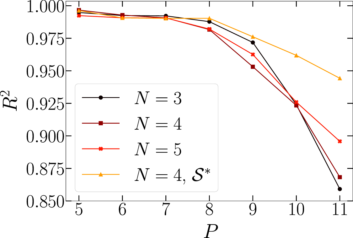
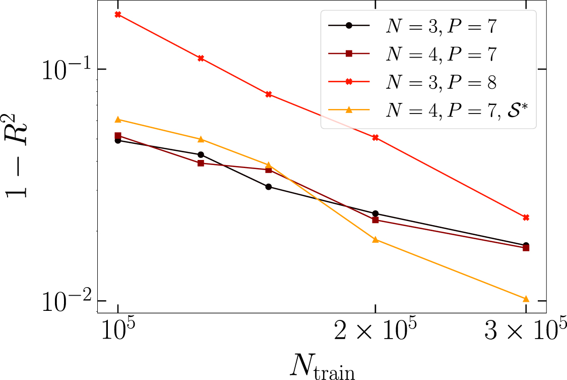
Figure A3. Single-qubit expectation values  predicted by the CNN versus the ground-truth results
  . The CNN is trained on (continuous) quantum circuits with
  qubits and tested on circuits with different number of qubits N: N = 20 with 2000 samples (a); N = 24 with 100 samples (
 ) (b). The color scale (blue to yellow) represents the absolute discrepancy
  . The (red) line represents the bisector
  .
.
Download figure:
Standard image High-resolution image