EVOLUTION OF RELATIVE MAGNETIC HELICITY AND CURRENT HELICITY IN NOAA ACTIVE REGION 11158

Current helicity and magnetic helicity quantitatively describe different aspects of a three-dimensional (3D) complicated magnetic field in solar atmosphere. Briefly, current helicity measures the local interlinkage of elementary current channels (Démoulin 2007) whereas magnetic helicity measures the overall complexity of the magnetic topology (Berger 1999). To investigate these two quantities, we need information on the 3D magnetic field from the photosphere to the corona which is, however, not directly accessible from observations but can be reconstructed using a technique called coronal field extrapolation.

The goal of this Letter is to derive the temporal evolution of current helicity and magnetic helicity using the observable photospheric magnetic field as boundary conditions to extrapolate the nonlinear force-free (NLFF) coronal magnetic field. Such studies are of primary importance in understanding the process of energy buildup and release for solar flares and coronal mass ejections (CMEs). Some attempts to determine magnetic helicity have been made recently, based on linear (Green et al. 2002; Leamon et al. 2004; Mandrini et al. 2005; Lim et al. 2007) or NLFF extrapolations (Régnier et al. 2002, 2005; Park et al. 2010). However, their results are limited by the inadequacies of either the photospheric-boundary data or the modeling of the coronal magnetic field. For instance, the linear force-free field is a rather restrictive assumption for the coronal magnetic field (Gary 1989); the low cadence and short time period leave important gaps in interpretation; and the small field of view (FOV) undermines the ability of reconstructing a realistic coronal magnetic field. Fortunately, full-disk, high-cadence and high-resolution photospheric vector magnetograms provided by the newly launched Helioseismic and Magnetic Imager (HMI; Schou et al. 2012) on board the Solar Dynamic Observatory (SDO) offers a good chance to advance such studies.

In particular, the notably flare-productive NOAA active region (AR) 11158 is well observed by HMI, near-continuously for a five day period of 2011 February 12–16 from its emergence through its flaring phase. The evolution of this AR is mainly characterized by two large bipoles emerging in close proximity and the strong shearing motion between the central sunspot clusters (Schrijver et al. 2011; Sun et al. 2012). Over the 5 day period, the AR hosts an X2.2 flare (with a peak GOES soft X-ray flux on February 15 at 01:56 UT) leading to a pronounced halo CME, 3 M-class and over 20 C-class flares. This AR has been a subject of intense research, and some interesting findings include: the fast sunspot rotation from 20 hr before to 1 hr after the X2.2 flare (Jiang et al. 2012); the flare-related enhancement in the horizontal magnetic field along the magnetic polarity inversion line (PIL; Wang et al. 2012; Liu et al. 2012) and the abrupt changes in Lorentz force vectors (Petrie 2012), the injection of oppositely signed helicity through the photosphere around the PIL (Vemareddy et al. 2012), etc. We hope that current helicity and magnetic helicity studied in the present Letter will add an additional piece of information to the puzzle of the flare/CME scenarios.

Current helicity is defined as the volume integral of $\textbf {B}\,{\bm{\cdot}}\, (\nabla \times \textbf {B})$, where B is the vectors of the magnetic field, and $\textbf {B}\,{\bm{\cdot}}\, (\nabla \times \textbf {B})$ is referred to as current helicity density h_c. In the present NLFF field model, h_c can be computed in all points in a volume, unlike previous works limited to $\textbf {B}_z\,{\bm{\cdot}}\, (\nabla \times \textbf {B})_z$ measured at the photosphere (Abramenko et al. 1996; Bao & Zhang 1998; Hagino & Sakurai 2004; Su et al. 2009) or single value of the force-free parameter, α ($\nabla \times \textbf {B}=\alpha \textbf {B}$), for a whole AR (Pevtsov et al. 1995). Furthermore use of the HMI vector data allows us to investigate, for the first time, the evolution of h_c at a cadence as high as 12 minutes.

Magnetic helicity is a well-conserved quantity in ideal magnetohydrodynamics (MHD) on large scales (Berger 1999). It is originally defined as the volume integral of $\textbf {A}\,{\bm{\cdot}}\, \textbf {B}$, where A is the vector potential of B, i.e., $\nabla \times \textbf {A}=\textbf {B}$. This original form is only applicable for flux-enclosed systems, i.e., $\textbf {B}\,{\bm{\cdot}}\,\hat{n}$|_S = 0 on the boundary S. In order to measure helicity in open systems such as the coronal magnetic field above an AR, a modified form with a reference field, relative magnetic helicity H_r, has been introduced (Berger & Field 1984). The most common choice of the reference field is the potential field. In this respect, H_r is written in the Finn–Antonsen form (Finn & Antonsen 1985):

$$\begin{equation} H_{r}=\int _{V} (\textbf {A}+\textbf {A}_{p})\cdot (\textbf {B}-\textbf {P})\,dV, \end{equation} \tag{ 1 }$$

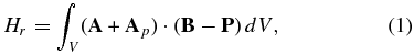
where P is the potential field that satisfies both $\nabla \times \textbf {P}=0$ and $\textbf {P}\,{\bm{\cdot}}\,\hat{n}$$|_{S}\,{=}\,\textbf {B}\,{\bm{\cdot}}\,\hat{n}$|_S, A and A_p are vector potentials of B and P, respectively. The modification renders the quantity gauge-invariant while maintaining its conservative property (Longcope & Malanushenko 2008).

On the other hand, one can gather information on helicity by evaluating helicity flux through the photosphere. Specifically, at a position $\textit {\textbf {x}}$ in the photospheric-surface S_ph and at a time t, helicity flux density $G_{\theta }(\textit {\textbf {x}},t)$ is given by (Pariat et al. 2005):

$$\begin{equation} G_{\theta }(\textit {\textbf {x}},t)=-\frac{B_{n}}{2\pi } \int _{S_{{\rm ph}}} \left(\frac{\textit {\textbf {x}}-\textit {\textbf {x}}\,^{\prime }}{|\textit {\textbf {x}}-\textit {\textbf {x}}\,^{\prime }|^{2}} \times [\textit {\textbf {u}}-\textit {\textbf {u}}^{\prime }] \right)_{n} B_{n}^{\prime } \,\hbox{\it dS}^{\prime }, \end{equation} \tag{ 2 }$$

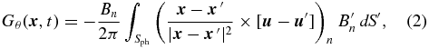
where the subscript n indicates the normal component to S_ph and $\textit {\textbf {u}}$ is the apparent horizontal velocity of magnetic footpoints at the photosphere. Practically $\textit {\textbf {u}}$ and thereby G_θ can be determined by tracking the apparent motion of the photospheric magnetic field with the local correlation tracking (LCT) technique or a newer one called the different affine velocity estimator (DAVE; Schuck 2006). Once G_θ is determined, the accumulated amount of helicity injection through the photosphere ΔH|_S is readily obtained by integrating G_θ with respect to area S_E and time t:

$$\begin{equation} \Delta H|_{S}=\int _{t_{0}}^{t} \int _{S_{E}} G_{\theta }(\textit {\textbf {x}},t)\,\hbox{\it dS}_{E}\,dt, \end{equation} \tag{ 3 }$$

where t₀ is the start time of the magnetogram series.

Two methodologies for measuring ΔH|_S and H_r are developed independently. Extensive studies of evolution of ΔH|_S have been conducted (Welsch et al. 2007; Park et al. 2010; Smyrli et al. 2010; Romano et al. 2011; Romano & Zuccarello 2011; Zuccarello et al. 2011; Vemareddy et al. 2012; Nindos et al. 2012) while the studies of evolution of H_r have thus far been rare. In this study, we explore H_r and h_c with the help of the advanced NLFF extrapolation method.

3.1. Data Set and Extrapolation

A series of photospheric vector magnetograms of the AR 11158 was provided by the SDO/HMI team. The data series is of 12 minute cadence (February 12–16) and 05 pixel⁻¹ resolution. Each vector magnetogram was disambiguated to fully determined 360° azimuth with the minimum energy method (Metcalf 1994; Leka et al. 2009), re-mapped and transformed to the Heliographic coordinate system using a Lambert equal area projection (Calabretta & Greisen 2002). The data products are described in more detail in http://jsoc.stanford.edu/jsocwiki/VectorMagneticField. Recently, Wiegelmann et al. (2012) examined the quality of the localized HMI vector magnetograms for the NLFF extrapolation and noted that (1) the FOV is large enough to cover not only the main sunspot clusters but also the diffuse, weaker-field surroundings, (2) the magnetic flux in this FOV is almost perfectly balanced, and (3) the net force and torque in the photospheric magnetograms are considerably smaller than that in other photospheric data obtained with earlier instruments, e.g., the Spectro-Polarimeter of the Solar Optical Telescope on board Hinode. All of these lay a good foundation for the subsequent NLFF extrapolation.

For the NLFF field extrapolation, we first rebin the data to 117 pixel⁻¹, and preprocess the data towards the force-free field condition (Wiegelmann et al. 2006). Then we apply the weighted optimization method (Wiegelmann 2004) to the preprocessed boundary to extrapolate the NLFF coronal magnetic field. The extrapolation is performed at 12 minute cadence and the dimensions of the computational domain are ∼217 × 217 × 170 Mm³. The metrics used to evaluate the quality of the extrapolation are given in Sun et al. (2012). One should be aware that NLFF field extrapolation is still in the experimental stage and the magnetic field topology reconstruction may vary with model (DeRosa et al. 2009). Thus helicities calculated with NLFF models should be interpreted with care.

Some samples of field lines from the resulting NLFF extrapolation are displayed in the left column of Figure 1, over the HMI vertical magnetograms. The rectangle marks the core region in a bipolar δ configuration that formed as a result of flux emergence. The most prominent shearing motion is seen in this core region. The field lines are color-coded according to their maximum altitude. The low-lying field lines (red) are in a sheared structure, whereas the high-arching lines (yellow) are potential-like.

Zoom In Zoom Out Reset image size

3.2. Current Helicity

The middle column of Figure 1 shows three snapshots of h_c at the altitude of 0.8 Mm deduced from the NLFF fields. An animation of 5 day evolution with 12 minute cadence is available in the online journal. The positive and negative h_c patches become clearly visible on February 13 as two bipolar regions emerge. The patch with positive h_c is mostly distributed over the inner bipole, while the negative h_c is seen in the immediate vicinity to the southeastern spots. The strong positive patch becomes S-shaped on February 14, that is always in alignment with the central PIL. On February 15, the patch with positive h_c evolves to an elongated structure connecting the opposite polarities of the inner bipole. The elongated structure starts to deform in shape on February 16, as the spots move apart.

The time–altitude diagram of average unsigned current helicity density 〈|h_c|〉, with the time profiles of unsigned magnetic flux (black-dashed) and GOES soft X-ray flux (black-solid), is shown in the top panel of Figure 2. The most striking feature in this diagram is the propagating ridge, that appears on February 13 and moves upward smoothly during the next two days. In the meantime, there is a continuous pumping of magnetic field from the subsurface to the corona, as implied by the steady increase of magnetic flux. The increase of magnetic flux and the upward propagation of 〈|h_c|〉 cease, about 6 hr and 1 hr, respectively, prior to the onset of the X2.2 flare. The propagating front is indicated by the white-dotted line, below which the accumulated value of 〈|h_c|〉 reaches 90% of the total at each time bin. The average speed of the upward propagation is estimated to be ∼36 ± 0.6 m s⁻¹. For comparison, the bottom panel shows the time–altitude diagram of magnetic energy density which we calculated by B² of the NLFF field. Most of the NLFF energy is concentrated below 10 Mm. Such a upward propagation pattern is also evident but with a higher propagation speed of ∼58 ± 0.7 m s⁻¹. The propagation shown in both panels suggests a gradual energy buildup for the X2.2 flare.

Zoom In Zoom Out Reset image size

3.3. Magnetic Helicity

To calculate H_r, we adopt the code of Fan (2009) to determine the vector potentials (A and A_p) based on the extrapolated field. The calculation of H_r is a highly demanding task, and is performed only at 2 hr cadence except the 8 hr period around the X2.2 flare for which the full 12 minute cadence is used. The right column of Figure 1 shows the examples of the vertically integrated product (A+A_p) · (B-P) (see an online animation for the five day evolution). Note that this product is not the real helicity density (Longcope & Malanushenko 2008), but shown here to indicate which region mostly contributes to the magnetic helicity integral H_r. Apparently the core region is mostly of positive helicity that increases with time. The negative helicity seen in the vicinity of the southeastern spots appears to display its strongest concentration on February 15 and fades out thereafter.

For a better illustration, Figure 3 presents the perspective and cutaway views of the product (A+A_p) · (B-P) on February 14, 22:00 UT. Inspection of Figure 3 immediately reveals the predominant role of positive helicity plays in this AR, especially in the core region. The positive helicity corresponds to the right-handed flux rope, which is a common feature in the southern hemisphere (Pevtsov & Balasubramaniam 2003).

Zoom In Zoom Out Reset image size

To calculate ΔH|_S, we first determine the horizontal velocity $\textit {\textbf {u}}$ by applying the DAVE method to a series of HMI line-of-sight (LOS) magnetograms of February 12–15 with 1 hr cadence. Here we bypass the data of February 16 in that the AR is located far away from the disk center on this day (∼S21W37), thus the projection effect in the LOS magnetograms is no longer negligible. Then we infer G_θ and ΔH|_S using the numerical method developed by Chae (2007). Figure 4 shows a sample of $\textit {\textbf {u}}$ and G_θ maps. Evidently helicity is injected from the subsurface with the emerging flux. In the core region, a negative patch appears along the PIL and between the positive patches on February 13 and 14, and nearly disappears on February 15 (Vemareddy et al. 2012).

Zoom In Zoom Out Reset image size

We can thus compare the temporal evolution of H_r and ΔH|_S obtained independently. As shown in Figure 5(a), the correlation between H_r and ΔH|_S is fairly good indeed. The dominant sign of helicity in both cases is positive, consistent with the hemispheric helicity rule (Pevtsov & Balasubramaniam 2003). Both the time profiles of H_r and ΔH|_S show an apparent increasing trend over time. The values of H_r and ΔH|_S are generally comparable, such that H_r is ∼5.8 × 10⁴² Mx² and ΔH|_S is ∼5.1 × 10⁴² Mx² ∼2 hr before the X2.2 flare. The good consistency between H_r and ΔH|_S shown here provides observational evidence in support of the helicity conservation from the subsurface to the corona.

Zoom In Zoom Out Reset image size

The uncertainties in H_r and ΔH|_S are estimated by taking only measurement errors into account. For HMI vector magnetograms, the spatial distribution of measurement errors is provided in each data. We add these errors to each data accordingly and redo the extrapolation and calculation, and find that the error-superimposed boundaries generally yield 10%–40% uncertainty in H_r. For LOS magnetograms, the measurement errors are typically ∼10 G. Thus we add a pseudo-random noise which has a normal distribution with a standard deviation of 10 G to each magnetogram, and repeat the calculation ten times. The uncertainty in ΔH|_S determined in this way is ∼0.5%. One should be aware that the actual uncertainty in ΔH|_S due to DAVE may be substantially larger than 0.5% (Welsch et al. 2007).

Note that there seems to be a temporal delay of the increase of ΔH|_S, i.e., magnetic flux and H_r increase first, and ΔH|_S follows along behind. It is very likely that this delay is not real, but merely due to the fact that neither DAVE nor LCT are able to measure the footpoint velocity of newly emerging magnetic fragments. Note also that both H_r and ΔH|_S keep on their increasing trend after the X2.2 flare. By examining the H_r and ΔH|_S maps, we identify that the increase occurs over the central core region presumably owing to the continued shearing motion after the flare.

This study presents two new phenomena: an upward propagation of current helicity density h_c prior to the X2.2 flare and so-called bump time profiles of relative magnetic helicity H_r before each of two major flares, M6.6 and X2.2, respectively.

We find the first phenomenon by tracing with time the height within which the majority of h_c is confined. This upward propagation of h_c is apparently related to the continuous pumping of magnetic flux from below and accumulation of magnetic energy entering into the corona. This propagation therefore corresponds to expansion of magnetic energy to higher altitudes, and indicates energy buildup in the corona. The X2.2 flare occurs ∼1 hr after this h_c propagation ceases.

The bump pattern in the time profile of H_r before each of two major flares is also a new phenomenon different from the monotonically increasing ΔH|_S prior to major flares (LaBonte et al. 2007; Park et al. 2008). This bump pattern could be found in this study thanks to the high cadence of the HMI data. An earlier work by Park et al. (2010) is indicative of a similar bump pattern of |H_r| before the X3.4 flare of the AR 10930, which was, however, unclear due to the cadence of Hinode vector magnetograms (typically 4–5 hr). Figure 5(b) shows the temporal variation of positive and negative helicity integrated over the volume in comparison with that of positive and negative photospheric magnetic flux integrated over the FOV. It is found that the bump time profile of H_r is due to local enhancement of positive helicity along with a monotonic increase of negative helicity. Specifically, the first bump is related to the initial flux emergence which largely carries positive helicity at the early stage of the AR growth and the subsequent injection of negative helicity in large amount around the central PIL. The second bump appears when the flux emergence is almost over and the AR develops its magnetic complexity by steady horizontal motions such as shearing and rotating sunspots (Jiang et al. 2012). It is such horizontal motions that supplied further positive helicity into the corona, leading to the increasing phase. Then a negative helicity patch along the PIL is suddenly enhanced (Vemareddy et al. 2012), which together with the decrease of positive helicity in the meanwhile underlies the decreasing phase. In contrast, the magnetic flux evolution as measured in the photosphere does not show the bump pattern.

A question is now which physical process produces the bump structure in helicity evolution. By comparing this observation with the helicity simulation by Kusano et al. (2003), we find a few similarities in that helicities in both signs locally enhance along the PIL, and annihilate each other to trigger magnetic reconnections. It is therefore likely that the H_r bump structure forms due to an injection of helicity followed by helicity annihilation. It is then puzzling why the H_r bump structure has a much longer period than time scales of magnetic reconnection implied by the flare X-ray light curves. In our speculation, the coronal magnetic helicity may evolve more gradually, and the associated magnetic field change triggers magnetic reconnections only when the magnetic system reaches a critical configuration. In this way, temporal evolution of H_r needs not be exactly synchronized with flares but must occur prior to them. This phenomenon is associated with the coronal magnetic field change, and may be apparent in the magnetic helicity evolution but not in the magnetic flux evolution as measured in the photosphere. We hope that future analysis of a larger set of vector magnetograms soon to be released by the SDO will help to verify our result and speculation.

J.J., C.L., N.D., Y.X., and H.W. were supported by the NSF under grants AGS 09-36665, 07-16950, 11-53424, by NASA under grant NNX 11AQ55G. S.P. was supported by KASI/Leading Science Project: Study on Effects of CME and High Speed Solar Wind on Near Earth Space. J.L. was partially supported by the WCU Program through NRF funded by MEST of Republic of Korea (R31-10016) and NASA grant NNX11AB49G. T.W. was supported by DLR-grant 50-OC-0501. Data are courtesy of NASA/SDO-HMI team. We thank P. Schuck for the DAVE code.