


ABSTRACT
As Voyager 1 and Voyager 2 are approaching the heliopause (HP)—the boundary between the solar wind (SW) and the local interstellar medium (LISM)—we expect new, unknown features of the heliospheric interface to be revealed. A seeming puzzle reported recently by Krimigis et al. concerns the unusually low, even negative, radial velocity components derived from the energetic ion distribution. Steady-state plasma models of the inner heliosheath (IHS) show that the radial velocity should not be equal to zero even at the surface of the HP. Here we demonstrate that the velocity distributions observed by Voyager 1 are consistent with time-dependent simulations of the SW–LISM interaction. In this Letter, we analyze the results from a numerical model of the large-scale heliosphere that includes solar cycle effects. Our simulations show that prolonged periods of low to negative radial velocity can exist in the IHS at substantial distances from the HP. It is also shown that Voyager 1 was more likely to observe such regions than Voyager 2.
Export citation and abstract BibTeX RIS
1. INTRODUCTION
Numerical implementation of time-dependent physical models of the solar wind (SW) interaction with the local interstellar medium (LISM) is of fundamental importance for understanding the structure of the heliosphere. Steady-state simulations, however complicated, are not capable of reproducing phenomena that vary on scales less than a solar cycle (∼11 years), and especially less than the Sun's rotation period (∼25 days). A realistic simulation requires knowledge of the plasma and magnetic fields as a function of time on a sphere around the Sun, the inner boundary conditions (b.c.'s), for an adequate simulation. This is a formidable task because we do not have sufficient observational data for such b.c.'s. The second half of the previous decade was characterized by a breakthrough in constraining the interstellar magnetic field (ISMF). The Solar Wind ANisotropy (SWAN) experiment on board the Solar Heliospheric Observatory made it possible to identify the direction of the LISM hydrogen (H) atom flow in the inner heliosphere (below 10 AU). Regardless of the actual accuracy in determining the direction of the neutral hydrogen atom velocity  and of the space orientation of the hydrogen deflection plane (HDP), the results reported by Lallement et al. (2005) channeled parametric simulations into a more realistic direction. The HDP is formed by the vectors of
  and
and  . The latter vector stands for the H atom velocity in the unperturbed LISM and is assumed to be parallel to the LISM velocity measured from the He atom distributions at Earth orbit (Moebius et al. 2004). The Interstellar Boundary Explorer (IBEX) is exploring the outermost reaches of the heliosphere from an orbit at 1 AU by measuring energetic neutral atoms created in the inner and outer heliosheaths (IHS and OHS). These sheaths are comprised of compressed, subsonic SW and LISM plasma flow on the inner and outer sides of the heliopause (HP).
The choice of the ISMF vector,  , in the HDP or slightly offset from it made it possible (McComas et al. 2009; Heerikhuisen et al. 2010; Pogorelov et al. 2011) to explain the correlation between the IBEX ribbon and the line of sights perpendicular to the magnetic field directions in the OHS behind the HP in the heliospheric model of Pogorelov et al. (2009b). Moreover, Heerikhuisen & Pogorelov (2011) have shown that the IBEX ribbon position on a sky map strongly correlates with the choice of the B − V plane, which is formed by the
  and
and  vectors. As illustrated in the simulation of Heerikhuisen & Pogorelov (2011), a choice of
  considerably offset from their B − V plane, which was nearly parallel to the HDP in Lallement et al. (2005), yields a ribbon that is considerably shifted from the observed position.
Voyager 1 and Voyager 2 crossed the heliospheric termination shock (TS) in 2004 December and in 2007 August, respectively (Stone et al. 2005, 2008), and are moving in the direction of the HP—a tangential discontinuity separating the SW from the LISM. They provide information about the local properties of the SW plasma at the heliospheric boundary. The Voyager 2 plasma instrument provides distributions (Richardson et al. 2009) that can be used to validate theoretical models and their numerical implementation (see, e.g., Borovikov et al. 2011). V1, however, can no longer measure plasma parameters, and a special algorithm has been developed for the plasma velocity reconstruction based the ion intensity anisotropy measurements using the Low Energy Charged Particle (LECP) instrument (Decker et al. 2010). Of great interest is the radial velocity, vR, profile derived from the LECP measurements after V1 crossed the TS (Krimigis et al. 2011). It exhibits a substantial negative time gradient of vR since mid-2007, so that vR has decreased to zero and ultimately acquired negative values. The explanation of such behavior is not easy (2011 Fall AGU abstracts by E. C. Roelof and L. A. Fisk & G. Gloeckler), if at all possible, in the framework of a steady-state plasma distribution. Pogorelov et al. (2009c) compared multi-fluid and MHD-kinetic simulations of the SW–LISM interactions for different B∞ and showed their qualitative agreement. Both models involve pickup ions created when interstellar hydrogen experiences charge exchange with the primary SW and LISM ions. This is done by solving the MHD system for a mixture of all charged particles. None of the steady-state simulations showed negative radial velocity components in the IHS. Moreover, since the V1 trajectory is away from the SW stagnation point on the inner side of the HP, negative velocities are unlikely even when V1 crosses crosses the HP penetrating into the OHS, unless the HP shape changes dramatically becoming normal to the SW flow.
It should not be surprising, however, that vR can be small or even negative in the presence of stream interactions in the IHS or if the HP experiences excursions in the heliocentric distance. The SW–LISM interaction is unsteady at different timescales, some of them related to periodic processes, such as the Sun's rotation and solar cycle, which always exist and affect the plasma distribution in the IHS. Near solar minima, the Sun's rotation produces corotating interaction regions (CIRs). Borovikov et al. (2012) have recently shown that this may result in complex plasma velocity distributions in the IHS, occasionally producing very low velocities. However, such regions are narrow and velocities are not negative. Note that V1 measured vR less than −20 km s−1 in the Sun's frame. Solar cycle effects, on the other hand, can produce features which persist for years (Pogorelov 1995; Tanaka & Washimi 1999; Zank & Müller 2003; Scherer & Fahr 2003; Izmodenov et al. 2005).
2. SOLAR CYCLE AND UNUSUAL SIGN OF THE RADIAL VELOCITY IN THE SW AND LISM
Pogorelov et al. (2009a) have demonstrated that the solar cycle can produce regions that have an unexpected sign in vR (negative in the IHS and positive in the OHS) extending nearly 20 AU from the HP into the SW region and up to 50 AU into the LISM. The inner boundary is fixed at 12 AU from the Sun, and the effect of CIRs is disregarded by assuming a sharp boundary between the slow and fast SW regions. It was assumed that during solar minimum, the slow SW occupies heliolatitudes −35° ⩽ θ0min ⩽ 35°. This region is then changed periodically as a function of time over solar cycle, reaching 80° at solar maxima. The SW velocity, density, and temperature in the slow region are VEs = 4 × 107 cm s−1, nEs = 8 cm−3, and 105 K, respectively. The parameters in the fast SW are VEf = 8 × 107 cm s−1, nEf = 3.6 cm−3, and 2.6 × 10⁵ K. The interplanetary magnetic field radial component at 1 AU is 28 μG. The vector  in the SW is assumed to be given by Parker's formula (Parker 1961) at the inner boundary. Our initial conditions thus correspond to solar minimum conditions. We also assume that the angle between the Sun's rotation and magnetic-dipole axes is initially α = αmin = 9° and changes sinusoidally, reaching 80° at solar maxima, where we allow the dipole axis to flip its orientation from one hemisphere to another. Thus, the polarity of the Sun's magnetic dipole has a 22 year period. To imitate the plasma characteristics in the V1 observations of the distant SW and in the IHS, we choose the direction at latitude θ = −40° in the meridional plane, where a region of negative vR was observed in Pogorelov et al. (2009a). This trajectory has a latitude exceeding the minimum latitudinal extent of slow SW. As will be seen from further discussion, there are other directions where negative vR can be observed, but the chosen one is the closest by the absolute value to the V1 trajectory latitude. Moreover, a virtual spacecraft can be chosen moving in the above direction with the velocity of the V1 spacecraft so that it crosses the TS at the time closest to the V1 crossing time within the solar cycle, and also observes negative vR. The variation of the plasma parameters along the chosen direction is best illustrated as a space–time plot. Figure 1 shows space–time plots of plasma number density (logarithmic scale) and magnetic field strength
  . The black curve identifies the line where vR changes sign from positive to negative. The black straight line shows a possible trajectory of a spacecraft moving at the V1 velocity (about 3.5 AU year−1). This trajectory does not coincide with the V1 trajectory and the comparison with observations is therefore qualitative. The HP and TS are clearly seen in both panels. The average heliocentric distance of the HP in the chosen direction is about 133.5 AU. The distribution of magnetic field shows a definite 22 year periodicity.
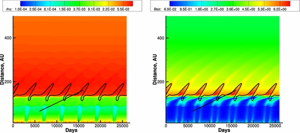
Figure 1. Space–time plots of (left) plasma density and (right) magnetic field magnitude in a direction imitating the Voyager 1 trajectory. The black curve shows the line where vR = 0. The black straight line is a possible trajectory of a spacecraft moving at the V1 velocity.
Download figure:
Standard image High-resolution imageTo understand the behavior of vR and magnetic field, in Figure 2 we show the linear distributions of those quantities as functions of heliocentric distance at fixed times: t = 10, 000 days (black lines) and t = 11, 732 days (red lines). The times given here are arbitrary and only time differences are meaningful, since they are defined by the solar cycle parameters. The radial velocity component becomes negative at R ≈ 113 AU and is positive again at R ≈ 133.5 AU, i.e., the width of the region with vR < 0 along the trajectory is about 20 AU immediately after solar minimum. Note that the magnetic field strength increases to more than 2 μG at the top of the barrier, which is qualitatively similar to recent V1 measurements (Burlaga & Ness 2012). Comparison of these two panels shows that there is a difference in the magnetic field behavior expressed in the red and black color. The red curve exhibits a gradual increase in  , or magnetic pressure, immediately after the TS. It appears that vR becomes negative approximately where B reaches the maximum. The region of increased magnetic pressure creates a form of magnetic barrier (cf. Nerney et al. 1993, who call such regions magnetic ridges, or Tanaka & Washimi 1999, who called them magnetic walls) that enhances the plasma deceleration. By contrast, ∼4.7 years before solar minimum, B starts decreasing behind the TS and the magnetic barrier attains a maximum at about 125 AU. The barrier being considerably narrower, it cannot substantially decelerate the SW plasma. It is worth noting that |B| has minima right in front of the HP in both cases, which is apparently due to the annihilation of the bipolar magnetic field characterizing an unresolved heliospheric current sheet (HCS). Magnetic barrier evolution is also clearly seen in Figure 1 (right panel). This barrier is not of the Nerney et al. (1993) type, who showed that magnetic barriers are naturally formed in the vicinity of the HP when magnetic field is compressed and field lines are carried away by the SW flow poleward. They exist in a spherically symmetric SW approximation (Pogorelov et al. 2004, 2006). They also exist in steady-state solutions with a fixed latitudinal extent of the slow wind. We used such steady state as an initial distribution in our solar cycle simulations (Pogorelov et al. 2009a). No steady-state solution of these kinds resulted in a negative vR along the Voyager trajectories. On the other hand, negative vR regions were observed by Washimi et al. (2011) in the time-dependent simulations based on the V2 plasma data in the assumption of a flat HCS and fixed latitudinal extent of slow wind (80°). According to available simulations, the mere presence of a barrier is insufficient to reverse the SW in the radial direction. Magnetic barriers that induce SW flow deceleration and reversal are due to solar cycle effects. The effect of the barrier reveals itself when regions of alternate magnetic field polarity are substituted by compressed monopolar field. This happens because of the interaction between streams that originate in the slow and fast wind regions. Near solar minima, what was originally the slow wind flows behind the barrier, while the fast wind flows on the other side. This is seen in Figure 3 which shows the evolution of the time-dependent barriers on the By plot in the meridional plane, as well as the SW "streamlines" (in which the out-of-plane velocity component is ignored). The lines start on a heliocentric circle belonging to the meridional plane. The regions with a very small and negative vR occur inside the HP where we see no streamlines or the streamlines look like vortices. The streamlines in these regions have substantial out-of-plane component. Although the absolute values of the HP excursions are not large (∼2.5 AU), they do accompany flow reversal regions in the IHS SW plasma. It is seen from Figure 1 that the HP stand-off distance increases slightly when negative vR is observed. This is due to the flow reflection from the HP and agrees with the global merged interaction region simulations in Pogorelov & Zank (2005), where it was shown that the largest SW flow reversals are observed at stages when the HP moves outward. This means that it is not the HP moving closer to the Sun that results in the SW flow reversals, and that the regions of negative vR are usually followed by those with positive radial velocity component.
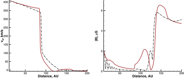
Figure 2. Linear distributions of the (left panel) plasma radial velocity component and (right panel) magnetic field magnitude at t = 10, 000 (black lines) and t = 11, 732 (red lines) before and immediately after solar minimum, respectively.
Download figure:
Standard image High-resolution image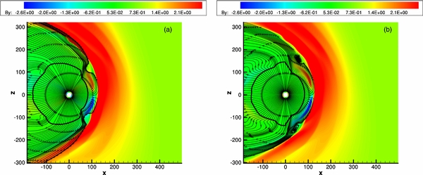
Figure 3. Evolution of the magnetic barrier in time. The streamlines start on the heliocentric circle of 15 AU radius and are shown neglecting the out-of-plane velocity component. The regions with no streamlines seen or vortices inside the HP are characterized by substantial magnitude of this component. The TS is shown with a thick black line. Distances are given in AU. The y-axis is directed into the figure plane.
Download figure:
Standard image High-resolution imageFigure 4 compares the SW radial velocity component along the chosen trajectory (the red line) and the V1 measurements (the blue line). There is a remarkable qualitative agreement between the calculated and measured distributions. There are two different slopes in both curves, the decrease in vR becoming steeper as the spacecraft enters the magnetic barrier. The simulation shows that vR should regain positive values which will continue until the spacecraft crosses the HP. The crossing will occur in about 4.5 years after the negative vR was observed. The HP asymmetry may add another ∼2 years.
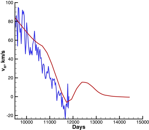
Figure 4. Distribution of the radial velocity component along the V1 trajectory from the spacecraft observation (26 day averages, blue line) and along the trajectory of a virtual spacecraft moving with the V1 velocity and crossing the region of negative vR.
Download figure:
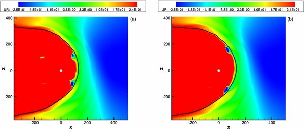
Standard image High-resolution imageThe regions of negative velocity originate in the IHS when the latitudinal extent of slow wind starts increasing after a solar minimum. Their intersection with the meridional plane is shown in Figure 5, but they apparently should have some longitudinal extent. These regions propagate latitudinally with the extent of the slow wind. This is seen in Figure 5, which shows the distribution of vR in the meridional plane for two snapshots corresponding to the SW–LISM evolution from a solar minimum to the following solar maximum. Note that the radial component inside the above-mentioned regions can acquire rather large negative values (as small as −35 km s−1). Spacecraft trajectories should be able to cross those regions to observe such small velocity values. For example, if we choose a straight trajectory at 50° latitude in Figure 5(a), a spacecraft moving along it will be able to see vR = −26.7 km s−1, vN ≈ 0.4 km s−1, and vT = −25.4 km s−1. Here we use the standard definition of the RTN coordinate system: the R-axis is directed radially away from the Sun, the T-axis is the cross product of the solar rotation axis and the R-axis, and the N-axis completes the right coordinate system. Note that the minimum latitudinal extent of slow wind is 35° in Pogorelov et al. (2009a), while it should be closer to ∼28° for the latest solar minimum and even smaller for the minimum following solar cycle 22. On the basis of these results, there is an explanation for why V1 is seeing large negative radial, nearly vanishing poloidal, and considerable transverse velocity components (Krimigis et al. 2011).
Figure 5. Changes in the distributions of the plasma radial velocity component with the increase in the latitudinal extent of slow wind. The snapshots are given at the same times as in Figure 3. The panel on the right shows a snapshot at a later stage after a solar minimum than in the left panel. The regions of vR < 0 expand poleward with the increase in the latitudinal extent of slow wind. Distances are given in AU.
Download figure:
Standard image High-resolution image
3. CONCLUSIONS
The Voyagers continue surprising us as they traverse the IHS and approach the HP. V1 observations of very small and then negative radial velocity components were accompanied by nearly zero latitudinal component, and a large transverse component. It appears that qualitatively very similar flow characteristics can be obtained if solar cycle effects are taken into account. Even the simplified solar cycle model by Pogorelov et al. (2009a) is capable of explaining many features of the observed plasma flow. Our simulations show that the radial component of the SW velocity in the IHS starts decreasing more rapidly once the plasma enters a magnetic barrier (plasma β inside the barrier is ∼5). These barriers lie outside the IHS region covered by the wavy current sheet. Since the magnetic field polarity changes every 11 years, our numerical simulations show a possibility of magnetic barriers of different polarity following each other. The width of the magnetic barriers and their ability to decelerate the SW flow are functions of solar cycle. Spacecraft approaching the HP may not necessarily see a negative vR. According to the solar cycle simulation discussed in this Letter, spacecraft can expect to start observing regions of low to negative radial velocity components shortly after a solar minimum. The reasons why V2 may not see negative radial velocities are as follows: (1) its velocity is less than V1 and (2) it crossed the TS later, within a solar cycle, than V1. As a result, the V2 trajectory is likely to miss the region of substantial negative velocity.
Plasma motions resulting in negative radial components of the SW velocity are mostly due to the time-dependent evolution of magnetic barriers in the IHS and are accompanied by minor excursions of the HP. We have shown that the regions of negative vR are time dependent and their spatial variation is closely related to the slow and fast wind interaction as the latitudinal extent of slow wind increases from solar minimum to solar maximum and monopolar magnetic field substitutes the bipolar field separated by the HCS. Slow and fast streams move on the opposite sides of the magnetic barrier, which makes their origin different from those proposed by Nerney et al. (1993). Negative vR is observed at the edge of the barrier when the plasma flowing on the barrier's outer side starts moving over it. Radial components can reach larger negative values at latitudes greater than the latitude of the V1 trajectory. The solar cycle model of Pogorelov et al. (2009a) discussed in this Letter is rather oversimplified, mostly because we assumed solar cycle and the excursions of the Sun's magnetic axes with respect to the equatorial plane to be strictly periodic (with the period exactly 11 years). This assumption is invalid for the latest solar cycle, which lasted almost 14 years, and was accompanied by a substantial decrease (by about 17%) in the SW ram pressure (McComas et al. 2008). For this reason, our numerical model cannot be applied to realistic Voyager trajectories, which made us consider virtual spacecrafts with the trajectories chosen so that they cross regions of negative vR on the SW side of the HP. This makes the results presented here qualitative. Furthermore, we chose the minimum latitudinal extent of slow SW to be 35°, which is not quite applicable to the latest solar minimum, where according to the Ulysses data it can be as small as 20°. As discussed above, there are regions in the SW where not only the radial velocity component is very small or negative, but also the latitudinal component nearly vanishes. As a result, the main SW motion can temporarily occur in the longitudinal direction. This is consistent with the Voyager observations published by Krimigis et al. (2011) and further measurements performed by V1 in 2011.
The authors are grateful to S. T. Suess for valuable comments. This work is supported by NASA grants NNX08AJ21G, NNX08AE41G, NNX09AW44G, NNH09AG62G, NNH09-AM47I, NNX09AP74A, NNX09AG63G, NNX10AE46G, NNX12AB30G, and NASA contract NNN06AA01C. Supercomputer time allocations were provided on SGI Pleiades by NASA High-End Computing Program award SMD-10-1691, Cray XT5 Kraken by NSF XSEDE project MCA07S033, and on Cray XT5 Jaguar by ORNL Director Discretion project PSS0006. This work was also supported by the IBEX mission as a part of NASA's Explorer program.