


ABSTRACT
We examine and reconstruct the interplanetary coronal mass ejection (ICME) first seen in space-based coronagraph white-light difference images on 2008 June 1 and 2. We use observations of interplanetary scintillation (IPS) taken with the Solar-Terrestrial Environment Laboratory (STELab), Japan, in our three-dimensional (3D) tomographic reconstruction of density and velocity. The coronal mass ejection (CME) was first observed by the LASCO C3 instrument at around 04:17 UT on 2008 June 2. Its motion subsequently moved across the C3 field of view with a plane-of-the-sky velocity of 192 km s−1. The 3D reconstructed ICME is consistent with the trajectory and extent of the CME measurements taken from the CDAW CME catalog. However, excess mass estimates vary by an order of magnitude from Solar and Heliospheric Observatory and Solar Terrestrial Relations Observatory coronagraphs to our 3D IPS reconstructions of the inner heliosphere. We discuss the discrepancies and give possible explanations for these differences as well as give an outline for future studies.
Export citation and abstract BibTeX RIS
1. INTRODUCTION
Coronal mass ejections (CMEs), their associated interplanetary counterparts, and the effects they cause on planetary environments are still not completely understood (e.g., Zhang et al. 2007). When a CME erupts from the Sun, it removes a large amount of mass (solar plasma) and magnetic energy and thrusts it out into the interplanetary medium, beyond coronagraph fields of view, where they become re-classified as interplanetary coronal mass ejections (ICMEs). In this Letter, we use the term CME to describe the 2008 June 1–2 event in coronagraph white-light imagery, and ICME when seen in heliospheric observations of interplanetary scintillation (IPS; e.g., Hewish et al. 1964; Cohen et al. 1967; Rickett & Coles 1991; Jones et al. 2007) and also in our heliospheric three-dimensional (3D) reconstruction later, in interplanetary space.
We use a time-dependent 3D Computer-Assisted Tomography (C.A.T.) algorithm incorporating a kinematic solar-wind model in order to reconstruct the inner heliosphere (out to 3 AU) in three dimensions in both density and velocity (see Jackson & Hick 2005; Bisi et al. 2009, and references therein). The 3D reconstruction results allow an isolation of the ICME from the background heliosphere and the ability to obtain an excess mass (CME/ICME mass) in the ICME volume above an assumed normalized background density of 5 electrons (e−) cm−3. The reconstruction uses observations of IPS taken using the Solar-Terrestrial Environment Laboratory (STELab) radio arrays, Nagoya University, Japan (Kojima & Kakinuma 1987). 3D reconstruction with our time-dependent model has a one-day cadence and 20° × 20° heliographic latitude–longitude digital resolution for the STELab IPS data used here. This resolution is primarily constrained by how many lines of sight are available for reconstruction. IPS is the rapid variation in radio signal from a compact distant natural radio source produced by turbulence and variations in the solar wind density. Density values for the solar wind can be inferred from the "scintillation level" (converted to the g level) of IPS observations using the method described in Jackson & Hick (2005), Bisi et al. (2008), and references therein.
Section 2 briefly describes the 2008 June 1–2 CME and mass determination using coronagraph imagery. Section 3 discusses the 3D reconstruction of the event, provides an IPS excess mass determination, and compares this excess mass to the coronagraph estimates. We discuss and conclude in Section 4.
2. OBSERVATIONS
The Solar and Heliospheric Observatory (Domingo et al. 1995)-Large Angle and Spectroscopic Coronagraph (SOHO|LASCO) C3 (outer coronagraph) instrument (Brueckner et al. 1995) first detected the CME (following an instrument outage) in Thomson-scattered white-light difference images on 2008 June 2 at around 04:17 UT. Its motion was tracked throughout a large portion of the C3 field of view. The resulting plane-of-the-sky velocity was 192 km s−1 according to the Coordinated Data Analysis Workshops (CDAW) CME catalog: http://cdaw.gsfc.nasa.gov/CME_list/. It should be noted that these measurements were labeled as having a quality index of "fair." The main CME feature had a position angle (PA) of 82° with an estimated angular width of the CME of 120°. An example difference image from LASCO C3 on 2008 June 2 at 10:19:58 UT is shown in Figure 1. The measured height–time (elongation–time) plot of this CME can be seen in Figure 2 using data taken from the CDAW CME catalog. Although the CME was recorded in the C2 instrument, measurements were only made in the C3 images from a height of 8 R☉ to 22 R☉.
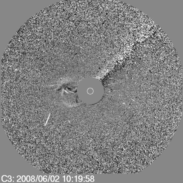
Figure 1. LASCO C3 difference image for observations of the 2008 June 2 CME showing its extent around half-way through this instrument's field of view of the event.
Download figure:
Standard image High-resolution image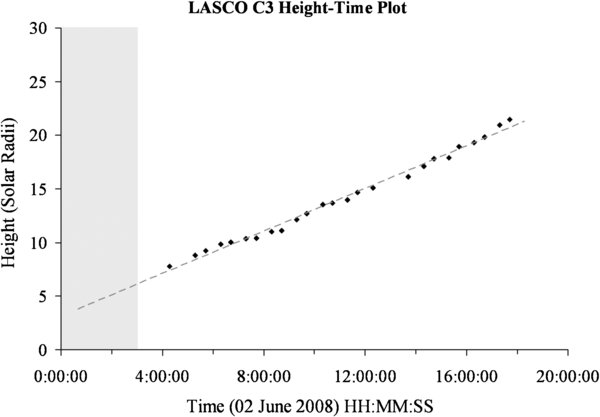
Figure 2. LASCO C3 height–time (elongation–time) plot of the 2008 June 2 CME using data taken from the CDAW CME catalog. The diagonal-hashed/gray area represents the time when LASCO was down until early on 2008 June 2; thus, measurements of the CME within the C3 field of view were only taken from a height of around 8 R☉ as noted in the text.
Download figure:
Standard image High-resolution imageThis event was discussed in detail by Robbrecht et al. (2009) as a "source-less" CME; meaning that no low-coronal signature in ultraviolet imagery could be associated with it or was left behind after the event. They concentrated on images from the Solar Terrestrial Relations Observatory (STEREO; Kaiser 2005; Kaiser et al. 2008) COR1 (inner) and COR2 (outer) coronagraphs. These coronagraphs form part of the Sun–Earth Connection Coronal and Heliospheric Investigation (SECCHI) instrument suite (Howard et al. 2008). The coronagraphs of the STEREO ahead (STEREO-A) spacecraft were used by Robbrecht et al. (2009) to obtain mass estimates of the CME in its early stages (see Table 1). The CME was seen in the COR-A imagery starting early on 2008 June 1. The CME width (angular extent) measured from the STEREO-A spacecraft was just 54° (Robbrecht et al. 2009). An extremely faint halo (front-sided) CME was also seen starting earlier in coronagraph imagery aboard the STEREO behind (STEREO-B) spacecraft, consistent with LASCO (and the COR-A instruments) seeing an east-limb CME from their perspectives. This adds as a possible explanation of why the CME width is smaller as viewed by the STEREO-A coronagraphs compared with the coronagraphs aboard SOHO (and the faint halo-type CME as observed by the STEREO-B coronagraphs) since limb events "look" smaller than halo events.
Table 1. Comparison of the CME/ICME Masses Obtained by Different Instruments/Methods
| Source | Excess Mass/CME Mass | Reference |
|---|---|---|
| CDAW CME Catalog (LASCO C3) | 4.7 × 10¹⁴ g | CDAW CME Catalog |
| STEREO COR1-A | 7.5 × 10¹⁴ g | Robbrecht et al. (2009) |
| STEREO COR2-A | 3.5 × 10¹⁵ g | Robbrecht et al. (2009) |
| STELab IPS | 1.4 × 10¹⁶ g | Our 3D Reconstruction |
Notes. Masses listed are actually excess masses from the ambient and are assumed to be the CME mass. In the case of the white-light coronagraph masses, these are obtained through difference images as described in Section 2. The 3D reconstructed mass from the STELab IPS data is obtained through isolating a volume assumed to be occupied by the ICME and then summing the mass above the ambient inside that volume as described in Section 3. Further details on what is considered ambient density in the reconstruction can also be found in the text.
Download table as: ASCIITypeset image
The mass determination of a CME in coronagraph images is typically undertaken using the methods described by Vourlidas et al. (2000) based on an earlier similar method by Poland et al. (1981). We include a brief overview of these in order to provide context to the coronagraph CME masses used in this Letter. The white light detected by coronagraphs is a result of scattered photons from coronal electrons, and transient activity such as a CME appears more intense and brighter in a coronagraph image than that of the ambient corona due to the increased density of electrons. Following calibration of the coronagraph images in units of solar brightness, a "pre-event" image containing the ambient corona in the region where the CME is detected is subtracted from subsequent frames where the CME appears. The excess number of electrons, and hence a mass estimate for the CME, is simply the ratio of the observed brightness over the brightness of a single electron at an angle (which is generally assumed to be 0°) from the sky plane. Using Thomson-scattering mathematics from Billings (1966) and an assumption of 10% helium abundance (which will result in 20% more electrons than protons), the mass is then calculated in grams (g) using Equation (1), where m is the excess mass, Bobs is the excess observed brightness, and Be(θ) is the brightness of a single electron at an angle θ from the sky plane (taken from Vourlidas et al. 2000):

After the mass image is obtained, the portion(s) of the images where the flux rope is located is(are) used, and the mass of the CME is obtained by computing the summation of the masses in the pixels within the flux rope (this is done by eye in general for the area in which the flux rope is within). Full details can be found in Vourlidas et al. (2000) and references therein.
3. THREE-DIMENSIONAL RECONSTRUCTION
The 3D reconstruction of the 2008 June 2 LASCO CME from the STELab IPS data shows the event with good clarity, particularly in the ecliptic plane on 2008 June 6 at 03:00 UT (as seen in Figure 3). This image shows a cut through the ecliptic as viewed from the north. The majority of the mass seems to be heading between Earth and STEREO-B at 1 AU distance, with more mass following mainly toward STEREO-B. This is consistent with both the LASCO and COR observations. Robbrecht et al. (2009) report that the STEREO-B measurements confirm that the ICME arrives at STEREO-B on 2008 June 6: our reconstruction confirms this (further investigation with in situ measurements will likely be the subject of a future paper). Our results discussed thus far are consistent with those of the previously mentioned work by Robbrecht et al. (2009) according to A. Vourlidas (2009, private communication).
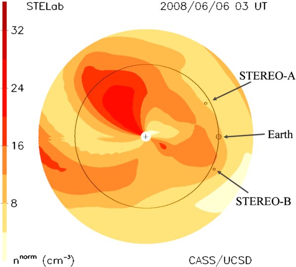
Figure 3. Cut through the ecliptic plane from the 3D tomographic density reconstruction as looking down from the north on 2008 June 6 at 03:00 UT. Marked on the image are the positions of Earth and the two STEREO spacecraft, as well as the near-circular orbital path of the Earth. The ICME can be seen heading between the Earth and the STEREO-B spacecraft and this trajectory is consistent with the estimated trajectory given in Robbrecht et al. (2009). We are not concerned with the far west and anti-Earth-ward ("backsided") features at this time. Additional explanations are given in the text.
Download figure:
Standard image High-resolution imageThe 3D tomography shows an unusually slow velocity for the ICME, approximately consistent with the LASCO height–time plot (Bisi et al. 2010). Although we do not present the velocity reconstruction here, it is important to remember such a slow-moving CME/ICME was most probably accelerated by the solar wind coming behind it through pressure build up (and thus likely to have mass added as it moves away from the Sun).
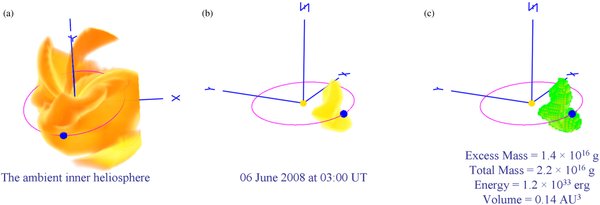
Figure 4(a) shows the 3D density structure of the inner heliosphere out to around 1.25 AU. The ICME is presently somewhat engulfed by the gross solar-wind structure somewhere to the east (left) of the Earth in this relatively complex, and relatively high-density overlapping/interlocking structure of the inner heliosphere at this time. The axes are heliographic coordinates with the X direction pointing toward the vernal equinox and Z toward solar heliographic north. The blue sphere represents the Earth (not to scale), and the purple ellipse the Earth's orbital path. A density of 10 e− cm−3 and upward is displayed showing the higher density assumed ambient portions of the inner heliosphere at this time. An r−2 density falloff has been removed (normalized to 1 AU) to better display structures at increasing distance from the Sun.
Figure 4. 3D density reconstruction volume from STELab IPS data on 2008 June 6 at 03:00 UT. The brighter the yellow-type color, the higher the density. (a) This shows the large-scale structure of the heliosphere as viewed from approximately 40° above the ecliptic and 10° west of the Sun–Earth line. (b) As in panel (a), but rotated around for clarity with non-ICME-associated features removed as described in the text; viewed from approximately 25° above the ecliptic and 40° east of the Sun–Earth line. (c) As in panel (b), but with the ICME portion from the STELab 3D reconstructed density volume highlighted (green cubes) indicating where the excess mass (assumed mass of the ICME) is in our reconstructed heliosphere. Full details can be found in the text.
Download figure:
Standard image High-resolution image
However, this convolution of structures can be resolved by cutting out parts of the reconstructed heliosphere thought not to be part of the ICME itself and viewing the volume from differing perspectives, being careful not to unnecessarily remove any portion of the 3D reconstructed ICME structure. The trimmed-down result can be seen in Figure 4(b) where a density of 12 e− cm−3 and upward is displayed. Here, the yellow/orange sphere represents the Sun at the center (not to scale). Finally, the volume of the ICME is determined in Figure 4(c). These show a 3D reconstructed view in density (this time out to around 1.1 AU with all non-ICME associated material/structure removed) but highlighted with cubes in Figure 4(c) to encompass the ICME's assumed volume. The ICME is relatively small in width (as with the STEREO-A COR observations) and extends to a greater height above and below the ecliptic (as with the LASCO C3 observations).
From the volume of the ICME in interplanetary space near 1 AU distance from the Sun, which in this case is 0.137 AU3, and the reconstructed density values present in each cube of the volume from the 3D reconstruction, the mass inside the volume encompassed by the cubes (the assumed ICME) is calculated. The total mass of the volume that we measure for the ICME is 2.2 × 10¹⁶ g, with an excess mass (to compare with coronagraph differenced-image values) above the ambient of 1.4 × 10¹⁶ g. We compare this measured value with other available excess masses obtained from the near-Sun white-light coronagraph difference images. All estimates are summarized in Table 1.
4. DISCUSSION AND CONCLUSIONS
The results presented and discussed here are comparing, for the first time, our 3D CME/ICME mass determinations with those of the STEREO coronagraphs. We also compare with the mass determination obtained from SOHO LASCO C3. This is the first set of comparisons with multi-viewpoint coronagraph imagery using the UCSD 3D tomography and acts as the initial stage for future more in-depth studies.
The different excess mass values obtained from the various instruments/techniques (Table 1) show a large variation. The LASCO C3 estimate is the lowest, with the inner and outer COR-A instruments getting progressively larger (respectively), and the STELab IPS reconstruction (much farther away from the Sun) giving the largest excess mass determination. Since the LASCO C3 view was more "front on" than that of the COR-A fields of view, we expect that more of the CME material is seen out of the plane of the sky from the LASCO point of view. Since in the difference imaging technique all material is assumed to be in the plane in the sky, this would lead to an excess mass estimate that is too low. The COR-A views are more "side on" than LASCO and thus they see a limb CME with more material close to the plane of the sky. The STEREO-A–SOHO separation angle at the time was around 27°. So it might be expected that, although the inner and outer COR-A coronagraphs have smaller fields of view than LASCO C3, both will still measure a larger excess mass than LASCO C3 (as is the case here). It should also be noted that the COR2-A excess mass measurement is a little over four times that of the COR1-A value. This is likely due to the CME gathering mass in its early stages of eruption and progressing out through the low corona. Robbrecht et al. (2009) note that the CME is "barely visible" in the COR1 imagery, but is much more clearly seen (brighter, and hence more massive) when it enters the COR2 field of view later on 2008 June 1. As noted previously, LASCO only saw the CME when it is further out from the Sun on 2008 June 2. This is a very slowly emerging CME, which, from the COR1-A mass depletion calculations after it leaves its field of view, was indicative of a partial streamer blowout (Robbrecht et al. 2009).
The STELab IPS 3D reconstructed excess mass result is around four times that of the excess mass measured by the COR2-A difference imagery. One contributing factor is that the ICME is seen in IPS much later near 1 AU when it is well developed and moving at a higher velocity. This suggests that it was accelerated by the higher-than-CME-speed solar wind behind it. This faster "ambient" solar wind adds mass to the CME/ICME and accelerates the ICME to speeds more consistent with the ambient solar wind speed. This likely caused an increase in pressure behind the ICME and thus would have "mass loaded" the ICME.
In addition, the excess mass determination from the IPS reconstruction works differently from that of white-light difference-imaging methods. In general, IPS is more sensitive to smaller-scale turbulent structure in the interplanetary medium, rather than Thomson-scattered white-light brightness; the latter is sensitive to the bulk density excess (as seen in coronagraph difference images). The IPS g-level is used as a proxy for density; this may not be always accurate due to the nature of IPS observations which are possibly more sensitive to density changes (and turbulence) than to density itself. Also, since there are many IPS lines of sight (and thus multiple viewing points as the ICME progressively makes its way from the Sun to around 1 AU) which are all used to formulate the reconstructed inner heliosphere during this time period, it is likely that a much larger extent of the ICME is being evaluated in the 3D reconstructed view than that of the two-dimensional (2D) plane as viewed by the coronagraphs. The 3D reconstructed mass should be larger for this CME/ICME as a result.
One other consideration is that since the total mass in the interplanetary medium at this time is relatively high (as seen in Figure 4), there is a possibility that we are also including some of the non-ICME material in our attempts to isolate the ICME and obtain an interplanetary excess mass measurement. These are all factors worth considering when evaluating the excess masses listed in Table 1.
In summary, the masses for the 2008 June 2 CME/ICME are somewhat different from each instrument/technique; larger masses further out from the Sun may reflect mass load behind the slow-moving CME but also highlight differences of the two observation types. In addition, it is difficult to isolate the ICME in the 3D reconstruction and be certain that the portion highlighted is just that of the ICME.
The additional detail here which may be able to reveal how and where the mass differences more precisely arise could come from looking at the 3D reconstruction of the ICME in greater detail and at differing distances from the Sun to near the Earth which is presently beyond the scope of this Letter but will likely be subject of a future publication. As well as this, with the fact that masses of CMEs from multiple coronagraph viewpoints can be obtained, a larger number of event studies with CME/ICME mass comparison will be useful to understand what and where the effects of the sky plane and material outside of the sky plane can vary the resultant mass value(s) obtained. Higher-resolution tomography using white-light Thomson-scattering brightness information from the Earth-orbiting Solar Mass Ejection Imager (SMEI) instrument may also yield a clearer insight into how and where the mass loading of slow CMEs, such as this one, occurs, with questions such as when the mass reaches its final mass, and what are the determining factors to accelerating the CME/ICME up to ambient solar wind velocity, among other possible investigations.
We acknowledge and thank the NSF (grants ATM0852246 and ATM0925023), NASA (grant NNX08AJ116), and AFOSR (grant FA9550-06-1-0107) for their funding. All SOHO images used in this Letter are taken from the Coordinated Data Analysis Workshops (CDAW) CME catalog http://cdaw.gsfc.nasa.gov/CME_list/. The CDAW CME catalog is generated and maintained at the CDAW Data Center by NASA and The Catholic University of America in cooperation with the Naval Research Laboratory. SOHO is a project of international cooperation between ESA and NASA.
Facilities: SOHO (LASCO) - Solar Heliospheric Observatory satellite, STELab - , STEREO (SECCHI) - NASA's Solar Terrestrial Relations Observatory