Abstract
We study the rate-independent decohesion process for a chain linked to a substrate through a series of breakable elements with a softening mechanism. Such an assumption describes the realistic case when connecting links can undergo softening transitions before breaking. For instance, this is a diffuse mechanism observed both in fracture of soft materials and biological adhesion. The analysis of this model is developed in the framework of equilibrium statistical mechanics. In order to describe mechanically induced detachment of the chain from the substrate both in the cases of hard devices (prescribed extension) or soft devices (applied force), we consider both Helmholtz and Gibbs ensembles. In any case, the model can be exactly solved and is characterized by a phase transition at a given critical temperature, corresponding to the complete detachment of the chain even without mechanical actions. Interestingly, according to the 'size' of the softened region, we observe two different regimes. In one case (fragile regime) during the decohesion the measure of the softened region is negligible, whereas in the other case (ductile regime) we obtain a finite measure of the softened region that is constant, giving a temperature dependent analytic measure of the process zone.
Export citation and abstract BibTeX RIS
1. Introduction
Micro-instabilities play a very important role in several artificial and biological mechanical systems. On one hand, concerning artificial systems, we can mention the peeling of a film from a substrate [1–7], the waves propagation in bistabile lattices [8–12], the energy harvesting through multistable chains [13–15], the plasticity and the hysteresis in phase transitions and martensitic transformations of solids [16–26] and the cracks and dislocations nucleation and propagation in materials and alloys [27–35]. On the other hand, micro-mechanical biological phenomena include the conformational transitions in polymeric and biopolymeric chains [36–49], the attached and detached states of fibrils in cell adhesion [50–55], the unzipping of macromolecular hairpins [56–61], the sarcomeres behavior in skeletal muscles [62–68] and the denaturation or degradation of nucleic acids, polypeptidic chains or other macromolecules of biological origin [69–78].
In all these physical situations we eventually find a multi-basin energy landscape and the state of the system can be in stable or meta-stable configurations, identified by the wells of the energy function. As a matter of fact, these systems are constituted by a large number of units characterized by two or more physical states. The transitions between these states or, equivalently, the exploration of the energy landscape, govern the macroscopic behavior of the whole system and, in particular, its static and dynamic features.
In a first class of systems, the intrinsic micro-instabilities may describe bistable units with transitions between one ground state and one metastable state (e.g. for the conformational folded-to-unfolded transitions in macromolecules or martensitic phase changes in metallic alloys). These types of transitions are typically reversible, which means that upon unloading the system follows the same path. Alternatively, in a second class of systems, investigated in this work, the micro-instabilities can model transitions between unbroken (attached) and broken (detached) states of breakable links (e.g. in the unzipping of hairpins, denaturation of macromolecules, fibrillar biological adhesion, peeling of films and cracks propagation). We underline that this kind of transitions can be reversible or irreversible depending on the considered physical system. For example, DNA denaturation is typically reversible whereas crack propagation is typically an irreversible process. In this work, as fully discussed below, since we do not consider cyclic loading, this difference is not crucial. On the other hand, because we refer to equilibrium statistical mechanics approach, we may fix our attention on reversible processes. Of course, the extension to irreversibility could be schematically described by introducing internal variables such as in [79] and assuming that each broken element cannot participate to the subsequent process.
The transitions between the states in all previous systems may be strongly influenced by thermal fluctuations, which can modify the probability of being in a given state or the passage rate between the neighboring energy wells. In particular, entropic energy terms can be relevant in transition and fracture phenomena of soft materials, such as biological and rubberlike materials [80, 81], or in the case of very low dimensional scales systems such as in shape memory nanowires [82]. In this context, the correct framework is the classical statistical mechanics. In particular, the systems exhibiting switching mechanisms between different energy basins can be studied by means of the spin variables approach.
The first theoretical approaches based on this method have been developed to model the biomechanical response of skeletal muscles [62, 63]. Then, this technique has been generalized to study different multi-stable systems [65–68], macromolecular chains [83–89] and phase transformations in nanowires [82]. This approach is based on the introduction of a series of discrete variables (similar to the spins used to deal with magnetic systems), which are able to identify the state associated with a given system unit. In other words, depending on the value of these discrete variables, the system transits between distinct energy wells possibly characterized by different position, shape, stiffness and depth. The introduction of the spin variables frequently simplifies the calculation of the partition function and the analysis of the corresponding averaged thermodynamic quantities. This technique has been largely exploited to investigate bistable systems with transitions between ground and metastable states, with important applications to nanomechanics [82–89]. Similarly, this approach has been considered for breakable materials with the spin variable distinguishing broken and unbroken units to study debonding processes in biological materials [27–29, 80]. In this paper, we introduce an important generalization of the model presented in reference [80], by including a softening mechanism in the breakable units of the system. More specifically, we study a one-dimensional lattice of masses linked by harmonic springs and connected to a substrate by breakable links subjected to a softening mechanism (see figure 1). This geometry has been previously introduced to describe a wide range of phenomena such as peeling of tapes, adhesion of geckos and denaturation of macromolecules [4, 5]. However, the thermal fluctuations and the softening mechanism have been neglected in these works, while in the physical systems recalled above they can play a crucial role that is analyzed in detail in the following development.

Figure 1. Scheme of the cohesion–decohesion process within both the Helmholtz (a) and the Gibbs (b) ensembles. While in the first case we prescribe the position yN+1 and we measure the average force  , in the second case we apply a force f and we measure the average position
  . In both cases, we consider a linear elastic behavior for the horizontal springs (c) and a breakable response with softening mechanism (d) for the vertical elements. The energy potentials W and U correspond to the horizontal and the vertical springs, respectively.
Download figure:
Standard image High-resolution imageFrom the mechanical point of view, we consider two different kinds of loading, which induce the decohesion of the system from the substrate. The decohesion process can be induced by either prescribing a given extension of the last element of the chain (figure 1(a)), or by applying an external force to the last unit of the chain (figure 1(b)). On one hand, the first isometric condition corresponds to the Helmholtz ensemble of statistical mechanics and can be generated by hard devices. On the other hand, the isotensional condition corresponds to the Gibbs ensemble and can be generated by soft devices. Indeed, these two boundary conditions can be deduced as limiting cases of real loading experiments, when the stiffness of the device is large (hard device) or is negligible (soft device) as compared with the loaded system one, respectively [88, 89]. From a theoretical point of view, an intriguing problem concerns the equivalence of the two ensembles in the thermodynamic limit (i.e. for very large systems) [90–96]. Interestingly, we will prove, in our case, the non-equivalence of the ensembles in the thermodynamic limit. Moreover, we are able to study the force necessary to detach the chain from the substrate as function of the temperature and of the external mechanical action applied to the system. In this context, we obtain a critical behavior described by specific phase transitions. Also the evolution of the number of intact, softened and broken elements is thoroughly investigated in both isometric and isotensional conditions. To conclude, the aim of this work is to fully analyze the cohesion–decohesion process with a softening mechanism in both the Helmholtz and Gibbs ensembles, thus providing a complete picture of the effect of the temperature and loading type on this prototypical physical system.
The paper is organized as it follows. In section 2 we define the problem and we simplify the spin variable methods through the zipper assumption. Then, in section 3, we introduce the system behavior under isometric condition, and in section 4, we analyze its thermodynamic limit. Similarly, in section 5, we introduce the system behavior under isotensional condition, and in section 6, we analyze its thermodynamic limit. The conclusions (section 7) and two mathematical appendices close the paper.
2. Problem statement
Our prototypical system is represented in figure 1. The horizontal springs of the lattice are purely harmonic, characterized by the elastic constant k (figure 1(c)), with a potential energy

On the other hand, the vertical ones can be in three different states, depending on their extension yi (figure 1(d)). When |yi | < yp , they are intact (elastic constant he ), when yp < |yi | < yb they are softened (elastic constant hp < he ), and when |yi | > yb they are broken (they do not support forces). This scheme represents the softening mechanism of the breakable bonds. We describe such a behavior in a spin formalism by introducing a discrete variable si associated to each vertical spring. Hence, we can write the potential energy of the breakable bonds in the form

where si
= +1 corresponds to the intact state, si
= 0 corresponds to the softened state, and si
= −1 corresponds to the broken state (i = 1, ..., N). With this assumptions we have a phase space composed on the N continuous variables  and the N discrete variables
  . Therefore, when we calculate the partition function, we have to integrate over all the continuous variables and to sum over all the discrete ones. So doing, the switching of the variable si
and their statistics at thermodynamic equilibrium are directly controlled by the statistical ensemble (Helmholtz or Gibbs in our case) imposed to the system.
. Therefore, when we calculate the partition function, we have to integrate over all the continuous variables and to sum over all the discrete ones. So doing, the switching of the variable si
and their statistics at thermodynamic equilibrium are directly controlled by the statistical ensemble (Helmholtz or Gibbs in our case) imposed to the system.
The assumption of considering independent spins for all the breakable bonds is the most rigorous approach to analyze the system behavior. However, on this assumption, the statistical mechanics of the system under investigation cannot be analytically developed and also its numerical implementation is quite expensive. Indeed, the calculation of the partition function is rather prohibitive because of the sum over all the possible spins combinations. Nevertheless, since we are studying the cohesion–decohesion process under an external mechanical action applied to one end point of the system, suppose the right one, we can simplify the model by assuming to have N − η broken elements on the right region of the chain, η − ξ softened elements on the central region of the chain and ξ intact or unbroken elements on the left region of the chain (see figure 1). In other words we suppose to have two moving interfaces or domain walls between the three regions of the chain. This hypothesis strongly reduces the mathematical complexity of the problem and is reasonable if we work at sufficiently low temperature and sufficiently large applied mechanical load (either extension or force). Indeed, the set of the three-state spin variables si
is substituted by the two variables η and ξ, assuming values in the set  . In this sense, η and ξ can be viewed as multi-valued spin variables. Moreover, this hypothesis is similar to the one adopted in the so-called zipper model, largely used to describe the helix-coil transitions in proteins, the gel–sol transition of thermo-reversible gels, and the melting or denaturation of DNA [97–100]. By implementing this simplified scheme, we deduce a fully analytical solution of both Helmholtz and Gibbs boundary problems for an arbitrary number N of elements of the chain, and also in the thermodynamic limit (N → ∞).
One of the most important result concerns the analytic expressions of the temperature dependent debonding force (or system strength) in both cases of isotensional and isometric loading. This temperature dependent behavior can be interpreted by observing that the thermal fluctuations may foster the decohesion, allowing the escape from the energy well shown in figure 1(d). More rigorously, we prove that this behavior can be explained in terms of a phase transition occurring at a given critical temperature. In particular, it means that the system can be completely detached from the substrate for supercritical temperatures even without any external mechanical action.
This behavior has been observed in several polymeric systems subjected to a force [101–103]. In particular, several important results have been obtained for the pulling processes of adsorbed polymers on a surface. They were found by means of directed or partially directed walk models of lattice polymers adsorbed at a surface under the influence of an applied force [104, 105]. In this context, a temperature-dependent critical force has been derived for semi-flexible polymers [106], polymers subject to an arbitrarily oriented force [107], heterogeneous adsorption surfaces [108], striped adsorption surfaces [109], and self-avoiding chains [110–112]. From a theoretical point of view, the main difference between these approaches and ours is that they use lattice polymers techniques whereas we adopt continuous geometric variables. Interestingly, the lattice methods can also describe bubbles with different physical states along the chain, without needing the zipper simplifying assumption. In our case neglecting such simplifying assumption would lead to a numerical treatment of the subject and we preferred the analytical clearness of the results. Importantly, in our continuous model we also introduced the softening mechanism, which is the main topic of this work and represents, as we show in the following, an important ingredient to distinguish different observed regimes in the decohesion behavior.
In our system, although the decohesion force for subcritical temperatures is the same for both statistical ensembles, they are not equivalent in the thermodynamic limit since the force–extension curves are different under isometric and isotensional conditions. Importantly, the softening mechanism in the breakable elements generates a strength-temperature curve composed of two branches connected, with continuity, at a given temperature T0. From the physical point of view, this is the temperature at which all the elements are at least softened. The interesting point is that this transition has been experimentally observed in the strength behavior of some systems including sapphire whiskers [30] and a number of high-entropy and medium-entropy alloys [32, 35]. In these cases, the softening mechanism is originated by the emergence of a population of dislocations beyond a certain threshold of deformation.
Another fundamental effect induced by the bonds softening is the possibility of describing a temperature dependent process zone that, for enough high temperatures, anticipates the propagation front. As a result we may obtain a transition between different regimes, experimentally observed for example in polymeric materials [113, 114].
Summarizing, the proposed system is particularly important for the following reasons: (i) once previous crucial assumptions are considered, the model can be analytically solved in both isometric and isotensional statistical ensembles; (ii) the solution shows a phase transition at a critical temperature that can be calculated in closed form; (iii) the studied system manifestly shows the ensembles non-equivalence in the thermodynamic limit, which is an unusual feature in statistical mechanics; (iv) finally, the model describe the existence of a two-branch curve for the strength-temperature behavior, observed in real materials, as a result of a softening anticipating breaking effects.
3. Hard device: Helmholtz ensemble
We consider the cohesion–decohesion process in the system represented in figure 1(a), where the detachment is generated by imposing the extension yN+1 of the last element of the chain. This condition corresponds to the Helmholtz ensemble of statistical mechanics and it is obtained in the case of loading with hard devices (with a very large, ideally infinity, intrinsic elastic constant). We identify the longitudinal springs with the potential energy  for any
  , and the transverse springs with the potential energy
  if |y| ⩽ yp
(intact),
if |y| ⩽ yp
(intact),  if yp
< |y| ⩽ yb
(softened), and
if yp
< |y| ⩽ yb
(softened), and  if |y| > yb
(broken). The values ±yp
of the extension correspond to the softening points A and B of the breakable spring, where the elastic constant switch from he
to hp
< he
. The force jump at y = ±yp
is given by
if |y| > yb
(broken). The values ±yp
of the extension correspond to the softening points A and B of the breakable spring, where the elastic constant switch from he
to hp
< he
. The force jump at y = ±yp
is given by  (see figure 1(d)). We simply calculate that
  , and we must always impose the inequality yb
> yp
, where ±yb
are the extensions at the breaking points C and D of the transverse elements. As anticipated, we assume that a first group of ξ elements of the chain are intact (i = 1...ξ), a second group of η − ξ elements are softened (i = ξ + 1...η), and a third group of N − η elements are broken (i = η + 1...N). These premises allow us to write the total potential energy of the system in the following form
, and we must always impose the inequality yb
> yp
, where ±yb
are the extensions at the breaking points C and D of the transverse elements. As anticipated, we assume that a first group of ξ elements of the chain are intact (i = 1...ξ), a second group of η − ξ elements are softened (i = ξ + 1...η), and a third group of N − η elements are broken (i = η + 1...N). These premises allow us to write the total potential energy of the system in the following form

where the applied extension yN+1 is considered as a parameter and we fix y0 = 0. The variables belonging to the phase space are the extensions y1, ..., yN and the two configurational numbers ξ and η, characterizing the state of the breakable elements. For further convenience, the energy function Φ can be further arranged as follows

where we defined the vector  , with each component representing the displacement of an element of the chain, the constant vector
  and the tridiagonal (symmetric and positive definite) matrix

We observe that ξ and η must fulfill the condition 0 ⩽ ξ ⩽ η ⩽ N. Moreover, this matrix has all the subdiagonal and superdiagonal elements equal to −1 and the diagonal elements defined as follows

where we introduced the rescaled elastic constants

The algebraic properties of the matrix  are studied in appendix
The equilibrium statistical mechanics of a system in contact with a reservoir at temperature T is described by the canonical distribution. In this context, the expectation values of physical observables can be obtained by evaluating the partition function that, within the Helmholtz ensemble, can be written as

where we have to integrate the continuous variables represented by the vector y , and to sum over the discrete variables ξ and η, describing the state (intact, softened or broken) of the elements of the chain (0 ⩽ ξ ⩽ η ⩽ N). Using equation (4), ZH can be evaluated using the property of Gaussian integrals

holding for any symmetric and positive definite matrix  . In particular, we can define
  and
and  to obtain

where

and  . We can thus determine the average force associated to the vertical extension yN+1 of the last element of the chain as [90]

We obtain

This expression represents the force–extension relation for the system within the Helmholtz ensemble, or equivalently, under isometric condition. It is also important to calculate the average value of the number of broken elements  and the average number of softened elements
  . These quantities can be directly evaluated through the expressions


In order to simplify the analysis it is useful to rescale the applied extension yN+1 with respect to yb (i.e. the extension corresponding to the breaking of the link) and define the non-dimensional extension

To simplify the formulas previously derived, we can consider the rescaled energies

Thus, introducing equations (16) and (17) into the expression of  ,
,  and
and  , we obtain


where we have used equations (10) and (11) to define the (rescaled) partition function

Using the properties of  and the relations in equations (A.18) and (A.19), it is possible to find explicit expressions for
  and
and  so to obtain the behavior of the relevant physical quantities of the system.
Previous results are represented in figure 2, where we study the dependence of the relevant quantities on temperature and size of the system. In particular, we plotted  ,
,  ,
,  and
and  versus the applied rescaled extension
  (changing the temperature) for two different cases: the first one concerns a short chain with N = 5 (panel (a)), and the second one a larger chain with N = 50 (panel (b)). For N = 5 (panel (a)), and for low values of the temperature, we easily identify the partial and complete rupture occurrences (see the peaks and/or steps in the curves of
  ,
,  ,
,  and
and  ). However, for larger values of the temperature, the curves are smoother because of the increasing thermal fluctuations. We also observe that the detachment of the elements of the chain occurs in a progressive way in response to the increasing extension
  . This is a specific feature of the Helmholtz ensemble, typically observed in the folding/unfolding process of bistable macromolecules stretched by hard devices [83–86, 88, 89]. For N = 50 (panel (b)), we can identify two important properties of the detachment process in large systems: first, increasing
  the curve approximately exhibits a temperature dependent plateau; second, during the decohesion process the number of softened elements is temperature dependent and approximately constant for small values of temperature in a certain range of
  . Although these features can be observed in the panel (b) of figure 2 only for low values of the temperature, we will deduce in the thermodynamic limit (i.e. when N → ∞) that this behavior can be explained in terms of a phase transition (see section 4). The existence of a constant finite softened domain shows the possibility of analytically describing the existence of a process zone regulating the advancing of the decohesion front as observed in cohesive fracture phenomena [113]. Interestingly, the size of the process zone increases with temperature, so that in accordance with the experimental behavior the decohesion is 'fragile' at low temperature and 'ductile' at higher values of the temperature [114].
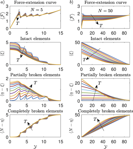
Figure 2. From top to bottom: force–extension curve and distribution of intact, softened and broken elements during the detachment of a film from a substrate for the Helmholtz ensemble (hard device, applied extension to the last element of the chain). Panel (a): we considered N = 5, and 10 values of KB T from 0.5 to 5 (a.u.). Panel (b): we considered N = 50, and 10 values of KB T from 2 to 20 (a.u.). The adopted parameters follows: he = 20, hp = 15, ΔE = 2, yb = 2yp and k = 5 (all in arbitrary units).
Download figure:
Standard image High-resolution image4. Thermodynamic limit within the Helmholtz ensemble
We study here the thermodynamic limit within the Helmholtz ensemble, defined by a very large number of elements in the chain (macroscopic limit valid for large systems). To this aim we have to study the behavior of equations (18)–(21) for N → ∞. In order to perform the analysis in this limit, we formally substitute the sums appearing in these expressions by integrals. In particular, we will use the approximation  for an generic function ϕ(χ). A better approximation could be adopted by using the Euler–McLaurin formula [115]. However, this approach, discussed in reference [80], is not necessary for the purposes of the present analysis. Moreover, due to the fact that we are considering the case of N large, it is possible to use the simplified expressions of
  and
and  , obtained in equations (A.22) and (A.23).
From equations (18) and (21) we get the following explicit result for the force–extension relation

where

To better understand the behavior of the force–extension response for large values of N, we firstly perform the integration on the variable ξ, and then apply the change of variable N − η + β0/(β0 − 1) = s, delivering the following result

The behavior of the previous expression depends on the sign of the quantity  , appearing in the exponential term within the square brackets in both numerator and denominator. From equation (17) we have

where we have defined the temperature T0, corresponding to a transition in the system behavior (we will prove that all elements are at least softened for T > T0). If T < T0 and we consider large values of N (thermodynamic limit), the exponential term in the square brackets of equation (24) is dominant. On the other hand, if T > T0 the exponential term in the square brackets of equation (24) is negligible for large values of N. Thus, for N → ∞ we obtain

and

In order to ensure the convergence of the integrals in equations (26) and (27) it is necessary that the following conditions hold


These conditions have a physical interpretation that will be discussed in the following.
The integrals appearing in equations (26) and (27) can be evaluated in terms of error functions as discussed in appendix

We thus obtain


It is possible to see that the quantities in the brackets in equations (31) and (32) converge to 1 when  . Thus, the expectation value of the force
  is characterized by an asymptotic force
  for large values of
  (coherently with figure 2(b)). In particular, we get the following asymptotic values

where

and

where

The parameters Tb
and Tc
represent two critical temperatures for the system with  in equations (33) and (35), respectively. As we will discuss in detail, it means that all the bonds are certainly broken for supercritical temperatures. These results also show that the conditions in equation (28), introduced to ensure the convergence of the integrals, correspond to requiring that the system is working at subcritical temperatures. It is possible to observe the emergence of two different cases depending on the parameters of the system. From equations (25) and (36), we find

As a consequence, we have

We remark that this analysis is valid if yb
> yp
, i.e. if the softening region exists. It is possible to verify the continuity of  for T = T0 from equations (33) and (35). As a matter of fact, from the definitions of T0, Tb
and Tc
in equations (25), (34) and (36) one can verify the equality
for T = T0 from equations (33) and (35). As a matter of fact, from the definitions of T0, Tb
and Tc
in equations (25), (34) and (36) one can verify the equality

Moreover, from this equality we obtain that

Thus, for the case with Tc
> T0 (i.e. when T0 represent the crossover temperature for the force–extension curves) in equation (38), the positivity of  implies that Tc
> Tb
> T0.
implies that Tc
> Tb
> T0.
This scenario is illustrated in figure 3, where equation (18) is compared, for a large value of N, with equations (33) and (35), corresponding to the thermodynamic limit. In order to show the effect of the condition in equation (38), we have fixed the values of the constitutive parameters but different values of the breaking extension yb
in the top and bottom panels (smaller value in top panels). This choice is reflected by the different size of the softening region of the potential energy U in panels (b) and (e). In panel (a) and (d) we plotted the force–extension curves from equation (18) for increasing temperatures and compared it with the asymptotic values obtained from equations (33) and (35). The good agreement observed proves that the theoretical procedure adopted to analyze the thermodynamic limit is correct and that the decreasing of the asymptotic force when the temperature increases is explained by the presence of a phase transition. The critical point depends on the constitutive parameters of the system. When  , we have that T0 > Tc
and, thus, the force–extension curve follows equation (33). As a consequence, the phase transition appears at the critical temperature Tb
. On the other hand, when
, we have that T0 > Tc
and, thus, the force–extension curve follows equation (33). As a consequence, the phase transition appears at the critical temperature Tb
. On the other hand, when  , we have T0 < Tc
. In this case, the force–extension follows equation (33) until the temperature reaches the value T0; when temperature is increased, the behavior of the force is described by equation (35) and the phase transition occurs at the critical temperature Tc
. From panels (c) and (f) of figure 3, we deduce that the force needed to obtain the complete detachment of the system monotonically decreases to zero for increasing values of the temperature. This process terminates at T = Tb
in panel (c), and at T = Tc
in panel (f). It means that the thermal fluctuations are able to promote the fracture of the breakable elements, and that the critical temperatures Tb
and Tc
are sufficient to induce complete denaturation of the system even if the resulting force experienced by the system is zero. This phenomenon can be better clarified by studying the behavior of
, we have T0 < Tc
. In this case, the force–extension follows equation (33) until the temperature reaches the value T0; when temperature is increased, the behavior of the force is described by equation (35) and the phase transition occurs at the critical temperature Tc
. From panels (c) and (f) of figure 3, we deduce that the force needed to obtain the complete detachment of the system monotonically decreases to zero for increasing values of the temperature. This process terminates at T = Tb
in panel (c), and at T = Tc
in panel (f). It means that the thermal fluctuations are able to promote the fracture of the breakable elements, and that the critical temperatures Tb
and Tc
are sufficient to induce complete denaturation of the system even if the resulting force experienced by the system is zero. This phenomenon can be better clarified by studying the behavior of  (average number of broken elements) and
  (average number of softened elements).

Figure 3. Behavior of the asymptotic force versus the temperature for a small (panels (a)–(c)) and a large (panels (d)–(f)) value of the breaking extension yb
. Panels (a) and (d): comparison between equation (18) with N = 300 (colored curves) and equation (33) (black straight lines) and (35) (red straight lines) at the thermodynamic limit (in panel (a), we used 8 values of T between 0 and Tb
; in panel (d), we used 10 values of T between 0 and Tc
). Panels (b) and (e): potential energy of the adopted breakable elements with different yb
(yb
= 1.5yp
in panel (b) and yb
= 3.5yp
in panel (e)). Panels (c) and (f): asymptotic force versus temperature (the green lines corresponds to equations (33) and (35); the circles to the colored curves of panels (a) and (d) for  ). The adopted parameters follows: he
= 20, hp
= 1, ΔE = 2, k = 5, and KB
= 1 (all in arbitrary units).
). The adopted parameters follows: he
= 20, hp
= 1, ΔE = 2, k = 5, and KB
= 1 (all in arbitrary units).
Download figure:
Standard image High-resolution imageWe will evaluate  and
and  in the limiting case of N → ∞. By performing the analysis used for the force–extension relation, starting from equations (19)–(21), we obtain


After the evaluation of the integral on ξ, we apply the change of variable N − η + β0/(β0 − 1) = s. We get


where we used  defined in equation (25). As for the force–extension relation, in the limit with N → ∞ we can consider separately the cases with Θ > 0 (T < T0, exponential term in the brackets is dominant) and Θ < 0 (T > T0, exponential term in the brackets is negligible). As a result, we get


We observe that the average number of softened elements  is independent of
  and is varying only with the temperature T for T < T0. It means that the two domain walls between intact and softened elements, and between softened and broken elements, move simultaneously with increasing
  conserving a constant distance between them (which means a constant number of softened elements). On the other hand, the value of
  is divergent to infinity when T > T0. This divergence means that we have no intact elements and the vertical springs can be either softened or broken. Therefore, the transition at the temperature T0 can be characterized by the partial breaking of all the elements of the chain induced by the thermal fluctuations.
The two integrals appearing in equations (45) and (46) can be calculated by using the formulas given in appendix

where the functions ϒ(λ) and Ψ(λ) are defined as follows


We can evaluate the asymptotic behavior of  for large values of
  for both T < T0 and T > T0. By means of previous results, and using the asymptotic expression
  for x → ∞, we easily get the asymptotic formulas for

The final asymptotic result can be therefore written as


This result shows that the increasing of the broken elements is linear with  (for
(for  large), confirming the progressive detachment process induced by the Helmholtz (isometric) condition. We can combine equations (33) and (35) with equations (51) and (52) to obtain the simple relation
  , which is valid for any temperature T, and for large values of the extension
  . This relation, rewritten in terms of the real physical quantities for large yN+1, reads

The behavior of the system within the Helmholtz ensemble in the thermodynamic limit is summarized in figure 4, where we plot the most important quantities versus the temperature by considering the two cases identified in equation (38). In particular, we fix the values of the constitutive parameters of the system but consider two different values of yb
. For small values of yb
(left panels) the temperature T0 is larger than Tb
and Tc
. Therefore, only the equations that are valid for T < T0 must be considered (panel (a)). On the other hand, for larger values of yb
(right panels), T0 is smaller that Tb
and Tc
: thus, the force–extension exhibits different regimes for T < T0 and T > T0 (panel (b)). In panel (a) (Tc
< Tb
< T0), the asymptotic force  shows a monotone decreasing behavior terminating at the critical temperature Tb
corresponding to a phase transition. The number of the softened elements
shows a monotone decreasing behavior terminating at the critical temperature Tb
corresponding to a phase transition. The number of the softened elements  is constant with respect to
  but is an increasing function of the temperature until the point A, corresponding to the phase transition. It means that the region of softened elements exhibits a fixed length and is gradually moved leftward by the increasing applied extension
  . The extension of this region represents the temperature dependent analytic measure of the process zone. Coherently, the number of broken elements
  is linearly increasing with
  and nonlinearly increasing with T (for this reason we plotted the ratio
  which is only temperature dependent). We observe that
  diverges at the critical temperature Tb
. Therefore,
diverges at the critical temperature Tb
. Therefore,  for T → Tb
for any value of the extension
for T → Tb
for any value of the extension  (for large values of
  ). It means that the phase transition can be explained through the total detachment of the system induced by the strong thermal fluctuations. In panel (b) (T0 < Tb
< Tc
), the asymptotic force
). It means that the phase transition can be explained through the total detachment of the system induced by the strong thermal fluctuations. In panel (b) (T0 < Tb
< Tc
), the asymptotic force  is a decreasing function of the temperature with a first transition at the point B (temperature T0) and a second final transition at temperature Tc
, where we have the complete detachment. The transition at T0 can be explained by observing the behavior of the number of softened elements
is a decreasing function of the temperature with a first transition at the point B (temperature T0) and a second final transition at temperature Tc
, where we have the complete detachment. The transition at T0 can be explained by observing the behavior of the number of softened elements  versus the temperature. We see that
  for T → T0, proving that all elements are (at least) softened for temperatures larger than T0. Therefore, we have the first transition at T0 where all the elements are softened, and a second transition at Tc
where all the elements are broken. This is coherent with the plot of
for T → T0, proving that all elements are (at least) softened for temperatures larger than T0. Therefore, we have the first transition at T0 where all the elements are softened, and a second transition at Tc
where all the elements are broken. This is coherent with the plot of  versus the temperature, from which we deduce that
  for T → Tc
for any value of the extension
for T → Tc
for any value of the extension  . The point C shows the slope transition in the evolution of the broken elements at the temperature T0. To complete the description of figure 4, we underline that the vertical dashed lines in all panels are useful to easily identify the characteristic temperatures Tc
, Tb
and T0. Moreover, the dashed curved lines correspond to solutions that are not relevant to the behavior of the system. More specifically, they correspond to equations (35) and (52) in panel (a) and to equations (33) and (51) in panel (b).
. The point C shows the slope transition in the evolution of the broken elements at the temperature T0. To complete the description of figure 4, we underline that the vertical dashed lines in all panels are useful to easily identify the characteristic temperatures Tc
, Tb
and T0. Moreover, the dashed curved lines correspond to solutions that are not relevant to the behavior of the system. More specifically, they correspond to equations (35) and (52) in panel (a) and to equations (33) and (51) in panel (b).
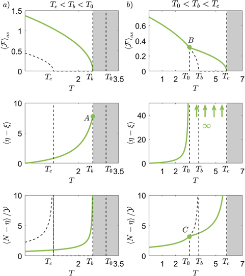
Figure 4. Behavior of the main quantities describing the system in the thermodynamic limit versus the temperature for a small (panels (a), where Tc
< Tb
< T0) and a large (panels (b), where T0 < Tb
< Tc
) value of the breaking extension yb
(yb
= 1.5yp
in panel (a) and yb
= 3.5yp
in panel (b)). In each case, we plotted the asymptotic or critical force  given in equations (33) and (35), the average number of softened elements
  , and the average number of broken elements divided by the applied extension
  . These plots correspond to the results given in equations (51) and (52). The shaded areas correspond to supercritical temperatures. The adopted parameters follows: he
= 20, hp
= 1, ΔE = 2, k = 5, and KB
= 1 (all in arbitrary units).
. These plots correspond to the results given in equations (51) and (52). The shaded areas correspond to supercritical temperatures. The adopted parameters follows: he
= 20, hp
= 1, ΔE = 2, k = 5, and KB
= 1 (all in arbitrary units).
Download figure:
Standard image High-resolution imageTo conclude, the behavior of the system under isometric condition can be usefully described by analyzing the phase diagrams represented in figure 5. Two cases are described: Tc
< Tb
< T0 (panel (a)); T0 < Tb
< Tc
(panel (b)). Observe that, since the system is symmetric (bilateral), in the figure we considered both positive and negative values of  . We can identify three possible phases for the system:
  corresponds to all the elements broken;
  corresponds to a combination of softened and broken elements; finally,
  corresponds to a mix of intact, softened and broken elements. These phases are separated by vertical lines corresponding to the phase transitions. Therefore, the phase diagrams explain clearly that, for Helmholtz isometric condition, we have no finite values of the prescribed extension
  able to induce the whole system detachment for subcritical temperatures. We will see that the Gibbs isotensional condition leads to a different behavior.

Figure 5. Phase diagrams for the system in the thermodynamic limit under Helmholtz isometric condition for the case with Tc
< Tb
< T0 (panel (a), where yb
= 1.5yp
) and for the case with T0 < Tb
< Tc
(panel (b), where yb
= 3.5yp
). We can identify three possible phases for the system:  corresponds to a phase with all the elements broken;
  corresponds to a combination of softened and broken elements; finally,
  corresponds to a mix of intact, softened and broken elements. The adopted parameters follows: he
= 20, hp
= 1, ΔE = 2, KB
= 1 and k = 5 (all in arbitrary units).
corresponds to a mix of intact, softened and broken elements. The adopted parameters follows: he
= 20, hp
= 1, ΔE = 2, KB
= 1 and k = 5 (all in arbitrary units).
Download figure:
Standard image High-resolution image5. Soft device: Gibbs ensemble
In this section we determine the properties of the detachment process realized within the Gibbs ensemble, which corresponds to a soft device able to apply a force to the last element of the chain. If we consider a force f applied to the last element with vertical extension yN+1, the total potential energy of the system is given by Φ − fyN+1, where Φ is the Helmholtz potential energy defined in equation (4). It follows that the Gibbs partition function is given by the Laplace transform of the Helmholtz partition function [92]. Moreover, the knowledge of the Gibbs partition function allows the calculation of the average extension of the last element of the chain by using classical thermodynamic relations [90]. We can introduce the non-dimensional quantities (analogous the those used in section 3)

representing the rescaled applied force and average extension, respectively. Thus, we can write the relations


We can easily determine the Gibbs partition function through equations (21) and (55) as a Gaussian integral. We obtain (up to a multiplicative constant)

where δ and φ have been defined in equation (17). By applying equation (56), we directly obtain the force–extension relation as

We can finally calculate the average value of the number of broken elements  and the average number of softened elements
  , eventually obtaining


An example of application of these results can be found in figure 6, where we plotted  ,
,  ,
,  and
and  versus the applied force
  (using the temperature as a parameter) for two different cases: the first one concerns a short chain with N = 5 (panel (a)), and the second one a larger chain with N = 50 (panel (b)). Concerning the case with N = 5, it is interesting to remark the differences between the Gibbs and the Helmoltz ensemble. We therefore compare the panel (a) of figure 2 with the panel (a) of figure 6. While the detachment of the elements is quite simultaneous within the Gibbs ensemble (cooperative process occurring at a given threshold force), the same phenomenon is sequential within the Helmholtz ensemble, where we observe a gradual and progressive bonds breaking (non-cooperative response). This different behavior is well known in the context of the stretching of macromolecules by means of force-spectroscopy techniques [83–86, 88, 89]. Another difference concerns the fact that in the Gibbs ensemble we are not able to identify peaks or steps in the curves of figure 6, corresponding to the single breaking occurrences. Also this point is clearly related to the cooperative response characterizing the Gibbs ensemble. If we look at the case with N = 50 (panel (b) of figure 6), we can see a well identified force plateau corresponding to the cooperative detachment of the elements. This force plateau is temperature dependent, as already observed within the Helmholtz ensemble. Moreover, we also deduce that the number of softened elements remains approximately constant and only temperature dependent before the complete rupture of the elements. These properties of the detachment process will be thoroughly analyzed in the next section, by introducing the thermodynamic limit of the Gibbs ensemble.

Figure 6. Force–extension curve and distribution of intact, softened and broken elements during the detachment of a film from a substrate for the Gibbs ensemble (soft device, applied force to the last element of the chain). Panel (a): we considered N = 5, and 10 values of KB T from 0.5 to 5 (a.u.). Panel (b): we considered N = 50, and 10 values of KB T from 2 to 20 (a.u.). The adopted parameters follows: he = 20, hp = 15, ΔE = 2, yb = 2yp and k = 5 (all in arbitrary units).
Download figure:
Standard image High-resolution image6. Thermodynamic limit within the Gibbs ensemble
In this section, we analyze the thermodynamic limit within the Gibbs ensemble and consider the behavior of equations (57)–(60) for N → ∞. Following the procedure shown in section 4 and using the formulas in appendix

where α0 and β0 have been defined in equation (23). After the integration over ξ we can apply the change of variable N − η + β0/(β0 − 1) = s thus obtaining

As before, this expression depends on the sign of the quantity  . In the limit with N → ∞ we consider separately the cases with Θ > 0 (T < T0, exponential term in the brackets is dominant) and Θ < 0 (T > T0, exponential term in the brackets is negligible). We eventually get (for N → ∞)


Finally, we obtain the force–extension formulas for N → ∞ under the same conditions for the Helmholtz ensemble (see equations (28) and (29)) as


We remark that these expressions reveal an asymptotic behavior corresponding to a force plateau, as already observed within the Helmholtz ensemble. In particular, the values of the asymptotic force are the same for the two statistical ensembles. Indeed, for T < T0, we deduce from equation (65) that the asymptotic force is solution of the quadratic equation  , which is exactly solved by the Helmholtz result stated in equation (33). Similarly, for T > T0, we deduce from equation (66) that the asymptotic force is solution of the quadratic equation
  , which is exactly solved by the Helmholtz result stated in equation (35). While the asymptotic forces are the same for the Helmholtz and Gibbs ensembles, it is not difficult to verify that the shape of the force–extension response is sensibly different for the two ensembles. This can be done by comparing the analytical solutions for the force–extension response obtained at the thermodynamic limit in equations (31) and (32) (Helmholtz) and equations (65) and (66) (Gibbs). It means that the two statistical ensembles are nonequivalent in the thermodynamic limit. For instance, this point can be shown by calculating the slopes of the force–extensions curves at the origin (for small forces and extensions) for both ensembles and by observing that these quantities are different. More details, concerning the case of the adhesion-decohesion process without the softening mechanism, can be found in [80].
To complete the analysis, we determine the average value of the number of broken elements  and the average number of softened elements
  in the limiting case of N → ∞. To this aim, we apply the same procedure already used for the force–extension relation. From equations (59) and (60), combined with the partition function given in equation (57), we obtain


After the integration over ξ and the change of variable N − η + β0/(β0 − 1) = s we obtain


where, as in section 4, we considered  . To complete the analysis, we consider the cases with Θ > 0 (T < T0, exponential term in the brackets is dominant) and Θ < 0 (T > T0, exponential term in the brackets is negligible). We get


These results can be used to understand the behavior of the detachment process within the Gibbs ensemble in the thermodynamic limit as shown in figures 7 and 8. In both figures, we have fixed the constitutive parameters of the model but the values of yb (small value in the left panel, larger value in the right panel). We recall that in the Helmholtz ensemble we obtained two different responses depending on the parameters, as stated in equation (38). In panel (a) of figures 7 and 8 we show the results for the case with Tc < Tb < T0 (yb = 1.5yp ), and in panel (b) those of the case with T0 < Tb < Tc (yb = 3.5yp ). While in figure 7 we show the behavior of the relevant quantities as function of the applied force (using the temperature as a parameter), in figure 8 we show the same quantities as function of the temperature (now using the applied force as a parameter).

Figure 7. Force–extension curve and distribution of softened and broken elements during the detachment of a film from a substrate with a soft device (Gibbs ensemble) in the thermodynamic limit. Panel (a): comparison of equations (57)–(60) with N = 250 (green dashed curves) and equations (65), (66), (71) and (72) obtained for N → ∞ (black solid curves) for the case with Tc < Tb < T0 (yb = 1.5yp ). We adopted 6 values of T between 0.4 and 2.4. Panel (b): comparison of equations (57)–(60) with N = 250 (green dashed curves) and equations (65), (66), (71) and (72) obtained for N → ∞ (black solid curves for T < T0 and red solid curves for T > T0) for the case with T0 < Tb < Tc (yb = 3.5yp ). We used eight values of T between 0.9 and 5.1. The adopted parameters follows: he = 20, hp = 1, ΔE = 2, KB = 1, and k = 5 (all in arbitrary units).
Download figure:
Standard image High-resolution image
Figure 8. Extension  , average number of softened elements
  , and average number of broken elements
  versus the temperature during the detachment of a film from a substrate with a soft device (Gibbs ensemble) in the thermodynamic limit. Panel (a): plots of equations (65), (66), (71) and (72) for different values of the applied force
  (eight values from 0.16 to 1.3) for the case with Tc
< Tb
< T0 (yb
= 1.5yp
). Panel (b): plots of equations (65), (66), (71) and (72) for different values of the applied force
(eight values from 0.16 to 1.3) for the case with Tc
< Tb
< T0 (yb
= 1.5yp
). Panel (b): plots of equations (65), (66), (71) and (72) for different values of the applied force  (10 values from 0.058 to 0.58) for the case with T0 < Tb
< Tc
(yb
= 3.5yp
). In both panels, shaded areas correspond to supercritical temperatures. The adopted parameters follows: he
= 20, hp
= 1, ΔE = 2, KB
= 1 and k = 5 (all in arbitrary units).
(10 values from 0.058 to 0.58) for the case with T0 < Tb
< Tc
(yb
= 3.5yp
). In both panels, shaded areas correspond to supercritical temperatures. The adopted parameters follows: he
= 20, hp
= 1, ΔE = 2, KB
= 1 and k = 5 (all in arbitrary units).
Download figure:
Standard image High-resolution imageIn figure 7 we draw a comparison between equations (57)–(60) with a large value of N and equations (65), (66), (71) and (72) obtained for N → ∞. This comparison prove that the mathematical treatment of the thermodynamic limit here developed is consistent with the model of detachment proposed. Indeed, we find a very good agreement between the general results, applied to system with a large value of N, and the theoretical ones obtained in the thermodynamic limit. Concerning panel (a), the force extension-curves exhibit the force plateau discussed above, which is very similar to the behavior observed within the Helmholtz ensemble. The average number of softened elements remains constant with  and depends on the temperature T. Finally, the number of broken elements diverges to infinity when the force approaches its critical value. The situation is more complicated in panel (b), where we have an intermediate transition describing the partial breaking of all the element of the system. In this case, when T < T0 (black solid curves), the behavior is very similar to the one described in panel (a). On the other hand, when T > T0 (red solid curves), all the elements are softened due to the thermal fluctuations and therefore
  (for this reason no red curves are shown in the plot of
  versus
  ). It means that the detachment process consists in the complete break of all the elements already softened.
Also in figure 8, we separately show the behavior of the system with Tc
< Tb
< T0 (panel (a) with yb
= 1.5yp
), and the system with T0 < Tb
< Tc
(panel (b) with yb
= 3.5yp
). We used a logarithmic scale to better appreciate the shape of the plots. The representation of the extension  , the average number of softened elements
  , and average number of broken elements
  versus the temperature is particularly useful to identify a crucial difference between the Helmholtz and the Gibbs ensembles. For the isometric condition (Helmholtz ensemble), we have no finite values of the prescribed extension
  able to completely detach the system for subcritical temperatures. Indeed, since the detachment progress is gradual or progressive in response to the prescribed extension, only an infinite value of extension can cause a complete detachment of the chain (see figure 4). Differently, for the isotensional condition (Gibbs ensemble), for any subcritical temperature, we can identify a value of force inducing the complete detachment of the chain. This can be seen by looking at the force–extension curves in panel (a) and (b) of figure 8. Here, we observe that for any value of the temperature, we can identify a force producing an asymptotic behavior of
  , which corresponds to the total detachment of the system. The relationships between force and temperature are given by
  for T < T0, and by
  for T > T0, as stated in equations (65) and (66) (we remember that δ and φ, defined in equation (17), depend on T). This is coherent with the fact that within the Gibbs ensemble all the element break simultaneously or cooperatively, thus allowing the force to completely detach the chain independently of the (subcritical) temperature of the system. The average number of softened elements
  is independent of the force and therefore we find a single curve (
 ) in the corresponding plot. However, for any applied force we have a different critical temperature of the system and then the curve of
  must be considered valid up to the red circle symbols shown in figure 8. Indeed, these symbols correspond to the critical temperature, which is, in turn, determined by the applied force. Finally, the curves of the average number of broken elements
  show a divergence at the critical temperature of the system, representing the complete detachment of the chain from the substrate. The important difference between panel (a) and panel (b) consists in the presence of the additional transition at the temperature T0 in the case with T0 < Tb
< Tc
(large breaking extension yb
= 3.5yp
). In this case, we observe that for T → T0 we have
show a divergence at the critical temperature of the system, representing the complete detachment of the chain from the substrate. The important difference between panel (a) and panel (b) consists in the presence of the additional transition at the temperature T0 in the case with T0 < Tb
< Tc
(large breaking extension yb
= 3.5yp
). In this case, we observe that for T → T0 we have  even if
  is finite. It means that at the temperature T ⩾ T0 all the vertical elements are spontaneously softened (due to the thermal fluctuations), and the detachment process is realized by completing their rupture thanks to the applied force.
To conclude the discussion concerning the thermodynamic limit in the Gibbs ensemble, in figure 9 we show the phase diagram of the system in the force–temperature plane. We separately considered the two cases with Tc
< Tb
< T0 (panel (a)) and with T0 < Tb
< Tc
(panel (b)). Again, due to symmetry, we considered both positive and negative values of  (see the scheme in figure 1 (panel (b))). Moreover, we observe the same three possible cases obtained in the hard device: the region
  corresponds to a phase with all broken elements; the region
  corresponds to a combination of softened and broken elements; finally, the region
  corresponds to a mixture of intact, softened and broken elements. In figure 9 we can identify the critical points (Cb
in panel (a), and Cc
in panel (b)), whose meaning is now quite clear: for temperatures larger than those of the critical points, the chain is always completely detached from the substrate. In panel (b) of figure 9 we can see the triple points P+ and P−, where the three phases of the system coexist. In any case, we observe that for a value of the applied force
corresponds to a mixture of intact, softened and broken elements. In figure 9 we can identify the critical points (Cb
in panel (a), and Cc
in panel (b)), whose meaning is now quite clear: for temperatures larger than those of the critical points, the chain is always completely detached from the substrate. In panel (b) of figure 9 we can see the triple points P+ and P−, where the three phases of the system coexist. In any case, we observe that for a value of the applied force  (in a suitable range), we have a value of the temperature able to detach the chain. When
  , such a temperature corresponds to the critical temperature of the system. In other words, for any subcritical temperature, we can identify a value of force inducing the complete detachment of the chain. As previously discussed, the critical behavior of the Helmholtz ensemble is different. In fact, for isometric condition, we have no finite values of the prescribed extension able to detach the system for subcritical temperatures, as shown in figure 5. This difference between the Helmholtz and the Gibbs ensembles is consistent with their non-cooperative and cooperative interpretation, respectively.
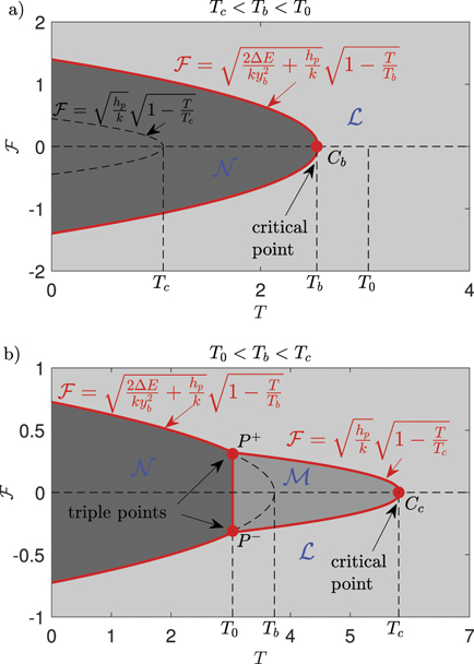
Figure 9. Phase diagrams for the system in the thermodynamic limit under Gibbs isotensional condition for the case with Tc
< Tb
< T0 (panel (a), where yb
= 1.5yp
) and for the case with T0 < Tb
< Tc
(panel (b), where yb
= 3.5yp
). We can identify three possible phases for the system:  corresponds to a phase with all the elements broken;
  corresponds to a combination of softened and broken elements; finally,
  corresponds to a mix of intact, softened and broken elements. We can also identify the critical points (Cb
in panel (a), and Cc
in panel (b)) and the triple points P+ and P− in panel (b), where the three phases of the system coexist. The adopted parameters follows: he
= 20, hp
= 1, ΔE = 2, KB
= 1 and k = 5 (all in arbitrary units).
corresponds to a mix of intact, softened and broken elements. We can also identify the critical points (Cb
in panel (a), and Cc
in panel (b)) and the triple points P+ and P− in panel (b), where the three phases of the system coexist. The adopted parameters follows: he
= 20, hp
= 1, ΔE = 2, KB
= 1 and k = 5 (all in arbitrary units).
Download figure:
Standard image High-resolution image7. Conclusions
We considered the cohesion/decohesion process under thermal fluctuations by means of a paradigmatic system represented by a linear mass-spring chain, connected to a substrate through breakable elements. These elements are described by a softening mechanism, i.e. by three operating regions as follows: the first linear region corresponds to intact elements (small deformation), the second region corresponds to softened elements with a reduced stiffness (intermediate deformation), and finally, the third region corresponds to broken elements (large deformation). This paradigmatic system has been studied under the assumption to be embedded in a thermal bath at a given temperature and to be loaded by an external mechanical action. This latter can be either a prescribed extension (hard device) or an applied force (soft device) to the last element of the chain. These two configurations correspond to the Helmholtz ensemble (isometric condition) and the Gibbs ensemble (isotensional condition) of the equilibrium statistical mechanics, respectively. In order to cope with the mathematical analysis of the problem, we adopted the spin variable approach for defining the state of any breakable element [83–86, 88, 89], we introduced the zipper model hypothesis with two domain walls for describing the three operating regions of the bonds chain [97–100], and we finally exploited some analytical properties of the tridiagonal matrices [116, 117] to obtain closed form results under isometric and isotensional conditions. In both cases we obtained the general solution of the problem for a chain composed of N elements. These solutions, in both cases, lead to a constant decohesion force, which represent the strength of the system. Importantly, this strength is temperature dependent, and its value is decreasing with an increasing temperature. The physical interpretation of this behavior can be done by observing that the thermal fluctuations foster the damaging of the breakable elements, thus reducing the strength of the system. Also the number of broken and softened elements have been determined as function of the temperature and of the external mechanical action for both statistical ensembles. Interestingly, we proved that the number of softened elements depends only on the temperature and it is independent of the external mechanical action. The increasing size of the softened region with the temperature gives a thorough interpretation of the fragile to ductile transition of several materials. This analysis provides a complete picture of the system behavior with a finite number N of elements. To better understand the meaning of these results, we analyzed the system behavior under the hypothesis of thermodynamic limit, i.e. for N → ∞. In this case, the sums appearing in the partition functions of both ensembles and in the macroscopic averages of the relevant thermodynamic variables can be substituted by integrals, eventually leading to useful closed form expressions. The analysis of these results delivers a clear explanation of the temperature dependent strength in terms of phase transitions. Indeed, a first critical temperature exists for the system and corresponds to the partial breaking of all the elements of the chain. Then, a second critical temperature describes the complete breaking of all the bonds. This complex critical scenario is able to give a rigorous explanation of the relationship between strength and temperature in system where a transition in the breaking mechanism occurs (here represented by the bonds softening). In several experimental measurements, a two-branch curve for the strength-temperature relation has been indeed observed [30, 32, 35]. Another interesting result concerns the non-equivalence of the ensembles in the thermodynamic limit. It means that the force–extension curves are different for the Helmholtz and the Gibbs ensembles, also for N → ∞. It is well known that the equivalence of the Gibbs and Helmholtz statistical ensemble has been proved for a large class of physical systems including, e.g. single flexible polymer chains without confinement effects and with a continuous pairing interaction potential between neighboring monomers [91–96]. However, it is difficult to prove the ensembles equivalence for more general systems or structures. For instance, other problems, concerning for example the escape of a polymer confined between two planes or the desorption of a polymer tethered on a surface, lead to the non-equivalence between the defined statistical ensembles [118–123]. Interestingly, these investigations are coherent with our results and definitively prove the possibility to have non-equivalence between different statistical ensembles in relevant physical systems. Generalizations of the theory may include the dynamic behavior of cohesion/decohesion processes (where the barriers between the wells of the energetic landscape play an important role [124–126]), or the multi-state softening i.e. composed of several steps with different stiffness (described by several domain walls in the chain).
Acknowledgments
GF and GP have been supported by the Italian Ministry MIUR-PRIN project 'Mathematics of active materials: from mechanobiology to smart devices' (2017KL4EF3). GF and GP are supported by GNFM (INdAM) and by the Italian Ministry MISE through the project RAEE SUD-PVP. GF is also supported by INFN through the project QUANTUM, by the FFABR research grant (MIUR) and the PON S.I.ADD. SG has been supported by 'Central Lille' and 'Région Hauts-de-France' under projects MePoFib and MiBaMs.
Data availability statement
No new data were created or analysed in this study.
Appendix A.: Properties of 

In this appendix we will recall some properties of tridiagonal matrices used in the text. In particular, we consider the matrix  defined in equation (5) and obtain the formulas for
 ![$\mathrm{det}\left[\mathcal{A}(\xi ,\eta )\right]$](https://content.cld.iop.org/journals/1751-8121/54/44/445001/revision2/aac2a07ieqn145.gif) and
and  .
.
For sake's of generality, let us consider  defined as

where the diagonal is composed by the elements (a1, ⋯, aN ), the superdiagonal by (b1, ⋯, bN−1) and the subdiagonal by (c1, ⋯, cN−1).
The elements of the inverse matrix  can be written as [116, 117]

where the sequences ϑi and φi are obtained using the recursive rules

and

Notice that while equation (A.3) is an increasing recursive rule going from i = 1 to i = N, equation (A.4) is a decreasing recursive rule for i = N to i = 1. It is possible to show [116, 117] that

These formulas can be specialized to the case where bi
= ci
= −1 ∀ i (such as for matrix  in equation (5)). The general result can thus be simplified as

where the sequences ϑi and φi are given by the reduced recursive laws

and

In order to evaluate the physical quantities in sections 3 and 5 we need to compute ![$\mathrm{det}\left[\mathcal{A}(\xi ,\eta )\right]$](https://content.cld.iop.org/journals/1751-8121/54/44/445001/revision2/aac2a07ieqn150.gif) and
and  . We have that

Let us consider equation (A.7) with a1 = ⋯ = aξ = 2 + α, aξ+1 = ⋯ = aη = 2 + β, and aη+1 = ⋯ = aN = 2. Then, for i ⩽ ξ we have the difference equation ϑi = (2 + α)ϑi−1 − ϑi−2, whose general solution can be written as

with Δ = α2 + 4α and where the coefficients p and q must be fixed using the conditions ϑ−1 = 0 and ϑ0 = 1. A straightforward calculation leads to the explicit solution for i ⩽ ξ

Let us define the function

which satisfies the properties  ,
,  , and
, and  . We can write the final result for i ⩽ ξ as

For ξ + 1 ⩽ i ⩽ η, we have the difference equation ϑi = (2 + β)ϑi−1 − ϑi−2, with the general solution

where Σ = β2 + 4β. In this case, the coefficients r and s must be obtained by imposing ϑξ−1 and ϑξ by means of equation (A.13). A long but straightforward calculation yields the final solution for ξ + 1 ⩽ i ⩽ η in the form

For i ⩾ η + 1, we have the simpler difference equation ϑi = 2ϑi−1 − ϑi−2, with the general solution ϑi = v + wi. In this case, the coefficients v and w must be obtained by imposing ϑη−1 and ϑη by means of equation (A.15). Hence, the result for i ⩾ η + 1 can be eventually found as

where ϑη−1 and ϑη are given by equation (A.15). The result for i ⩾ η + 1 can be therefore written in the following final form

From equation (A.9) we finally find

and

These formulas are used in sections 3 and 5.
The function  defined in equation (A.12) can be simplified by observing that the second term is defined by a power with a base always strictly less than one. Thus, for large values of z, the second term can be neglected with respect to the first one. More specifically, we have two different cases:


These results can be used to simplify equations (A.18) and (A.19) leading to


These expressions are used to evaluate the formulas in sections 4 and 6.
Appendix B.: Calculation of useful integrals
In order to develop equations (26) and (27) in closed form we have to consider the integrals

where a and b are two real and positive constants. For obtaining an explicit expression for these integrals, we define the quantities

We can therefore write

Now, we can observe that

and hence, we can write equation (B.3) in the form

To conclude, by remembering the definition of the error function [115]

we can observe that

and we directly obtain the first important result

Since from equation (B.2) we have that  and
and  , we get the final results


The two integrals appearing in equations (45) and (46) can be developed by evaluating

Since

we get the relation

Therefore, we easily obtain

This expression allows to write the final result in the form