

Abstract
We develop a microscopic approach to the kinetic theory of many-particle systems with dissipative and potential interactions in the presence of active fluctuations. The approach is based on a generalization of the Bogolyubov–Peletminskii reduced description method applied to the systems of many active particles. It is shown that the microscopic approach developed allows us to construct the kinetic theory of two- and three-dimensional systems of active particles in the presence of nonlinear friction (dissipative interaction) and an external random field with active fluctuations. The kinetic equations for these systems in the case of a weak interaction between the particles (both potential and dissipative ones) and low-intensity active fluctuations are obtained. We demonstrate particular cases in which the derived kinetic equations have solutions that match the results known in the literature. In addition, analysis of particular solutions showed that in the case of a friction force linearly dependent on the speed of structural units, the manifestation of self-propelling properties in the process of evolution of an active medium may be due to the local nature of active fluctuations.
Export citation and abstract BibTeX RIS
1. Introduction
Active matter is a field in soft matter physics that studies the properties of aggregates of self-propelled objects that have the ability to take up energy from the environment, store it in an internal depot, and convert internal energy into kinetic energy. Active matter comprises diverse systems spanning from macroscopic (e.g. schools of fish and flocks of birds) to microscopic scales (e.g. migrating cells, motile bacteria, and gels formed through the interaction of nanoscale molecular motors with cytoskeletal filaments within cells). Here we refer the reader to the reviews [1–4] and references therein. In recent years the number of publications devoted to theoretical and experimental studies of the phenomena in active substances has sharply increased, and some recent achievements have been published in the Special Issues of the European Physical Journal Special Topics and the Journal of Statistical Physics [5–9]. The study of nonequilibrium processes in systems of active particles inevitably raises the question of the consistent derivation of the evolution equations for such systems, in particular, the kinetic equations. The derivation of a kinetic theory of active particles is a challenging issue that has attracted significant attention over the past decades. Bertin et al [10–12] has derived the Boltzmann equation for self-propelled point-like particles on a two-dimensional plane with the assumption that the modulus of the velocity vector is fixed and identical for all particles so that only the direction of the vector plays a role in the dynamics. Ihle [13, 14] developed an alternative kinetic approach that is based on the Chapman–Kolmogorov equation for the N-particle probability density. The resulting mean-field kinetic equation has been studied analytically and numerically, and has been extended to the so-called topological interactions [15–17]. Romanczuk et al [18–20] derived and explored the mean-field kinetic equation in two spatial dimensions, starting from the Langevin equation with active friction and active fluctuations, and supplemented with different forces describing the interaction between the particles. In [21], the authors also pursue the Langevin approach to study collective dynamics in the two-dimensional system of active Brownian particles with dissipative interactions.
In this paper we develop a consistent microscopic approach based on the reduced description method of relaxation processes. The reduced description method of Bogolyubov–Peletminskii has a number of notable advantages. In particular, it allows one to formulate approaches for the construction of the kinetic theory of systems of many identical particles, and thus, in essence, provides a dynamic justification of the statistical mechanics of such systems [22, 23]. Bogolyubov suggested a method of reduced description of the evolution of many-particle systems [22], which allowed the construction of a regular procedure for obtaining closed dissipative kinetic equations based on the Bogoliubov–Born–Green–Kirkwood–Yvon (BBGKY) chain of reversible equations for many-particle distribution functions. Fundamentals of the reduced description method were formulated in [22] for the classical (nonquantum) systems of many particles. In the case of quantum many-particle systems, the ideas of the Bogolyubov reduced description method were developed in the works by Peletminskii, and the main results were presented in [23]. There are also other approaches for the dynamical justification of statistical mechanics that are different from Bogolyubov's approach; for example, in the works of Prigogine's Brussels school [24], as well as the different formulations of Bogolyubov's ideas, see, e.g. [25–28]. In the present paper we use the reduced description method in the form close to the one of Bogolyubov–Peletminskii [29] to construct the kinetic theory of many-particle systems with active fluctuations and nonlinear friction. For that purpose we need to generalize the canonical Bogolyubov–Peletminskii approach in order to take into account an external stochastic impact and dissipative interactions.
A generalization of the Bogolyubov reduced description method to the case of dissipative many-particle systems in an external stochastic field was first suggested in [30]. In this paper, the authors proposed a formalism for deriving kinetic equations. As a starting point, a stochastic Liouville equation obtained from Hamilton's equations taking dissipation and stochastic perturbations into account was used. The Liouville equation is then averaged over realizations of the stochastic field by an extension of the Furutsu–Novikov formula to the case of a nonGaussian field. As a result, a generalization of the classical Bogolyubov–Born–Green–Kirkwood–Yvon hierarchy is derived. In order to get a kinetic equation for the one-particle distribution function, the authors use a regular breaking procedure of the BBGKY hierarchy by assuming weak interaction between the particles and weak intensity of the field. Within this approximation they get the corresponding Fokker–Planck equation for the system in a nonGaussian stochastic field. Two particular cases assuming either Gaussian statistics of external perturbation or homogeneity of the system are discussed. In that approach, however, the stochastic external forces do not depend on the velocity (or momentum) of the particles. In other words, the formalism developed in [30] can be applied to systems with nonlinear friction, as is the case of active particle systems, but with passive fluctuations of either Gaussian or nonGaussian nature.
As mentioned above, we announce this work as one in which a general microscopic approach is proposed based on the first principles of statistical physics for the construction of the kinetic theory of such complex systems as dissipative media with active fluctuations. These media are proposed to be considered in the manuscript as systems of many identical particles. The structural units of the system are assumed to be point-like, but capable of reacting to an external stochastic effect depending on the magnitude and direction of their own velocity. This is their main individual characteristic, indicating that the point particles have the property of the so-called head–tail asymmetry. In particular, the manifestation of the self-propulsion property of the medium itself can be associated with just this simplest characteristic of the asymmetry of structural units. In this paper, we show that in the studied model of the active medium the self-propulsion property can manifest itself as a collective effect; however, its very manifestation is possible only due to the individual properties of the structural units of the system, i.e. the active particles.
Actually, one of the main goals of this work was to demonstrate both the necessity and the very possibility of developing a microscopic approach for building the kinetics of such complex systems with as accurate formulations as possible. In addition, we wanted to unite the existing phenomenological approaches (if possible, without contradictions) with their generalization to a number of more complex systems with active fluctuations. First of all, this means the correct inclusion of potential and dissipative interactions between the structural units of the systems under study. In parallel, we aimed to take into account the possibility of influencing the system of spatially correlated noise depending on the absolute value and the direction of the velocity of the system's structural unit. At the same time, the formulations should allow for a generalization of the approach to the case of nonGaussian noise. All stated goals could be achieved only within the framework of a microscopic approach based on the first principles of statistical physics. In this sense, we consider reference works [22–27] with a preference for strict approaches and elegant formulations of the monograph [23]. This means that the scheme for constructing the microscopic approach should contain a series of consecutive, strictly controlled steps. In particular, based on the individual equations of motion for the structural units of the system, the Liouville equation must be obtained for the distribution function of all the particles of the system. From the Liouville equation, the transition must be made to the equations of motion for many-particle distribution functions, which will have the form of an infinite chain of kinetic equations, which, in essence, is a generalization of the BBGKY chain to the case of systems with active fluctuations. The next step in the procedure for constructing a kinetic theory is the controlled truncation of this chain in any perturbation theory. In the present article we choose the weak interaction between the structural units of the system and the low intensity of the external stochastic force as the small parameters for such a perturbation theory. In this case, the density of the system is not necessarily small, and the closed kinetic equation for the single-particle distribution function has the form of the Fokker–Planck equation. Recall that, in accordance with [23], it is also possible in perturbation theory to break an infinite chain of equations—an analogue of the BBGKY chain and in the case of low medium density and with arbitrary interaction between particles, but only if this interaction does not lead to the formation of bound states. In this case, we would inevitably come to some analogue of the Boltzmann kinetic equation. However, for the active media under study, the possible (in principle) implementation of this case leads to significant mathematical difficulties and requires separate efforts (see this in regards [31]). Note also that in the transition from the Liouville equation to an infinite chain of equations, an additional intermediate step is required. It is connected with the necessity of averaging the Liouville equation, obtained from the initial equations of motion for structural units, over an external stochastic field. In this case, the work in [30] described above becomes useful, and its technique is easily modified for the systems studied in this article.
Building a consistent microscopic approach requires, first of all, to go beyond the Langevin equations as the initial equations of motion for the structural units of the system (see in this regard [30]). Instead of the Langevin equations, it is necessary to formulate the generalized Hamilton equations, that is, to start from the first principles of classical theoretical mechanics. Within the framework of such formulations it is possible to correctly include the interaction between structural units, both potential and dissipative. In this case, there are no problems with the inclusion of velocity-dependent noise correlated both in time and in coordinates. Note that the proposed theory does not deny the possibility of incorporating the Langevin equations as the initial equations of motion for structural units of the active medium. However, it will not be possible to talk about a rigorous microscopic theory that comes from first principles. In fact, the Langevin equations themselves were originally obtained as phenomenological equations of motion (Newton's equations), in which the force of the medium on a selected (test) particle is divided into a regular friction force and some random force. Thus, the Langevin equations are formulated for obviously noninteracting particles. For this reason, the inclusion of interaction between particles in these equations is again associated with the involvement of phenomenological approaches. Note also that in the 'traditional' Langevin equations, the noise acting on Brownian particles depends only on time and not on the coordinates. The presence of spatially correlated noise in the Langevin equations in the existing methods for deriving the Fokker–Planck kinetic equation would lead to serious mathematical difficulties. Thus, in accordance with the requirements listed above, the task of describing kinetic processes in the systems under study is posed in the most general form possible.
The solution of this problem in the present work is also carried out in the most general and consistent form, adhering to the first principles of statistical physics. First of all, this refers to the derivation of general kinetic equations for a system of active particles. Of course, a number of successive simplifications were used in this paper, connected with the transition from more complex systems, for which more complex equations were derived. In particular, we completely refused in the present work the generalization of the proposed approach in the case of nonGaussian noise. First of all, it was done for the sake of reducing the volume of the article. In addition, such a simplification is possible because, in light of [30], the ways of modifying the approach proposed in this article to the case of nonGaussian noise seem quite understandable and do not contain fundamental difficulties. The paper also carried out a fairly detailed analysis of some more simple specific examples, designed to demonstrate the effectiveness of the proposed method and the kinetic equations obtained in terms of the implementation of the announced goals. Such efficiency is most easily illustrated by analyzing cases in which the results of our theory coincide with or are close to the results of other authors obtained in other approaches. Section 6 of this paper is fully devoted to the solution of the latter problem, in which the results of the analysis of some particular solutions of our equations are given.
Thus, as the result of the consistent implementation of the above tasks, we suggest a generalized formulation of the reduced description method, suitable for describing the kinetics of many-particle dissipative systems with active fluctuations. It is shown in the framework of the microscopic approach developed that it is possible to construct the kinetic theory of active particles in both two- and three-dimensional systems, with the availability of nonlinear friction (dissipative interaction), as well as with local impact of an external active random field. Under the local impact we assume that this field may act differently at different points in space. In other words, the effect of this field on a particle may depend not only on the velocity (or momentum) of that specific particle, but on the point in the coordinate space where the particle is located. The general kinetic equations for such systems are obtained. We also consider special cases in which the obtained kinetic equations give solutions known for the active particles from earlier works [3, 18, 20, 21].
2. Basics
Consider a system consisting of N identical active particles of mass m, each of which is characterized by spatial coordinates  ,
,  , measured from the center of mass, and momentum
  ,
,  . The interaction between the particles is assumed to consist of two parts—a 'reversible' part described by the Hamiltonian H, and an 'irreversible' one, described by the function
  , the meaning of which will be explained below.
The Hamiltonian of the system can be written as follows:

where  is the pair interaction potential,

We also assume that the particles of the system are exposed to specific forces that depend on the particle velocity (or momentum) and are characterized by a function R. We assume that the function R can be represented as

where  is a regular part of this function.
and  is a stochastic part of the function R, which can be written as
The stochastic nature of the function  is formally highlighted by the presence of index
  .
.
Note that in the case of nonactive identical particles with the dissipative interaction function,  is treated as a dissipative function (see [32] and [30, 31]). It is usually assumed that the dissipation in the system is related to friction of macroscopic particles. Therefore, in this case the dissipation function
  , following [32], can be chosen as

This implies that  if
if  , where r0 is a characteristic range of dissipative forces. In view of the property (5) the friction coefficient is always positive.
However, in the case of active particles the positivity does not always hold [3]. The friction coefficient in the Langevin-type equations for active particles can depend on the velocity and change its sign. Therefore, one cannot use the criteria (5) to determine the properties of dissipation function  in the case of active particles.
Following the usual classical theoretical mechanics procedures, and taking into account equations (1)–(4), the generalized Hamilton equations for the system under study can be written as

Thus, the force  acting on a particle
  from the particle
  consists of two terms:

Namely, the force  , connected with the presence of a potential pair interaction between the particles, and the force
  , connected with the presence of a dissipative interaction between the particles (in the sense outlined above):

In addition, the  th particle is influenced by external random force
  (see equation (1), which depends on the momentum of the particle, wherein
The latter expression requires some comments. We emphasize, first of all, that the stochastic force  in equation (9) is written in a form that is not related to the choice of a particular coordinate system. This notation simply reflects the fact that the stochastic force acts differently along and across the direction of a particle velocity. Figure 1 shows a schematic visualization of the assumption written in the form (9). Expression (9) looks like a natural extension of the stochastic force
  typical for the Langevin equation in the case of an ordinary Brownian particle:

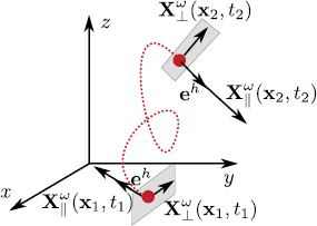
Figure 1. Schematic visualization of particle motion in the presence of stochastic effects with components  ,
,  according to equation (9).
Download figure:
Standard image High-resolution imageIn fact, the value  in the last equation can always be identically rewritten as

where  is an arbitrary unit vector, for example,
  . Replacing here the scalar product
  with
with  ,
,  by
by  , and assuming that
  , we arrive at equation (9). It should be remembered, however, that in equation (9) the values
  ,
,  do not relate to each other in general. If necessary, in the three-dimensional case the vector
  can be considered as two-component in a plane perpendicular to the vector
  . The presence of components
  along
along  will not affect the description of processes and phenomena in such systems in any case because of the factor
  in the right-hand side of equation (9).
It follows from the above that the stochastic effects on the system under consideration in the form of equation (9) can be regarded as a generalization of stochastic forces used in the theory of two-dimensional systems of active particles, i.e. active fluctuations; see, e.g. [3, 18]. First, equation (9) allows for the possibility of local influence of stochastic forces on the system. Second, equation (9) can be applied to both two- and three-dimensional systems as well. To see this it is sufficient to consider expression (9) as two-dimensional and nonlocal:

where  is a unit vector along the direction of motion of a particle,
  is a unit vector along the azimuthal angle
  , and
, and  and
and  are angular and velocity noise intensities, respectively [3]. Note that in two-dimensional systems, as is known, the isolated directions can appear in the movement of active particles. The special importance of the direction of particle motion, set by the particle's orientation vector (head–tail axis) is due to the existence of the propulsion mechanism. Thus, due to the head–tail asymmetry in the steady state of the many active particles system it is possible to fix the reference system in a natural way by a special choice of the vectors
  ,
,  . The existence of this asymmetry is reflected in the many-particle system characteristics, such as a one-particle distribution function. As shown below, the existence of the effects of head–tail asymmetry is also possible in three dimensions, even in the case of linear friction (see section 5 of this paper). We emphasize that the source of stochastic effects can be generalized to three dimensions in a form other than that in equation (9). Similar to the two-dimensional case, one can use the spherical coordinates. However, in this paper it is easier to employ the Cartesian coordinates.
Let us also note the following. The time derivative of the total energy of the system in accordance with equations (1) and (6) is given by

If we assume that the system has a dissipation due to friction of macroscopic particles, and a regular part of the dissipation function  is given by equation (5). Then, equation (11) together with equation (9) give

or
Taking into account that  (equation (5)), competition between the dissipation due to friction and the pumping of energy from the stochastic field is possible in such a system.
A further task is to obtain the Liouville equation. To this end, and for the convenience of further calculations, we represent equation (6) in the following form

where we introduce the notation

Thus, equation (13) together with equations (14) and (5) read

where

The coordinates and momenta of the  th particle at time t (see equation (14)), are determined by the coordinates and momenta
  of all the particles at the initial time t = 0:

where the functions  and
and  satisfy the generalized Hamilton equation (5) (or equations (13)–(16)). We introduce the probability density

 of the initial conditions
  ,
,

Then, at time t the probability density  ,
,  , (N-particle distribution function) is defined by the expression

In [33] a detailed procedure for obtaining the Liouville equation for many-particle systems in an external stochastic field neglecting the interaction between the particles is described. In [30] (see also [33]), a similar procedure is used to obtain a generalized Liouville equation for dissipative many-particle systems in the absence of an external stochastic field. The N-particle distribution function obeys the continuity equation

where the function  is given by expressions (16) and (17). This is the Liouville equation generalized to the case of active particles with pair interactions under the influence of external stochastic fields depending on the velocities of the particles. With equations (13)–(16) equation (20) can be written as follows:
In what follows we will use the Liouville equation (21) transformed with equations (13)–(16), (8), and (9) to the form
where  and
and  are determined by equations (7)–(9). Equation (22) is an example of the evolution equation with multiplicative noise. Now, the goal is to average this equation over realizations of the external random force
  .
.
3. Averaging the generalized Liouville equation with Gaussian random force
We introduce the N-particle distribution function  , which is the distribution function
  (see equation (19) averaged over the random external field
  with probability density
 ![$ W [ {\mathbf Y} ^ {\omega}] $](https://content.cld.iop.org/journals/1751-8121/52/44/445001/revision2/aab3f45ieqn068.gif) :
:
By using the averaging operation (23) for equation (22), we obtain
To have a closed evolution equation for the introduced distribution function, it is necessary to express the value of  through
  . We use the so-called Furutsu–Novikov formula [34, 35], which was proved for the case of Gaussian distributions of the external random field. For nonGaussian random fields, the Furutsu–Novikov formula is generalized in [29] (see also [30]). In this article, we will not recount the latter proof, and refer the reader to the works cited above. We use the result of the proof in [29] in the case of a Gaussian distribution of multiplicative noise. Thus, we get
where  ,
,  and
and  is a pair correlation function of the external Gaussian noise (
 ):
):

In what follows we use  . Now, let us consider
in more detail. We assume that the pair correlation function  is different from zero in the interval
  . We also assume that when
  , the pair correlation function
  has a sharp maximum. Then the functional derivative
 ![$ \frac {\delta D ^ {\omega} [ {\mathbf Y} ^ {\omega}]} {\delta Y_{j} ^ {\omega} \left (x ', t' \right)} $](https://content.cld.iop.org/journals/1751-8121/52/44/445001/revision2/aab3f45ieqn080.gif) is to be evaluated only at
is to be evaluated only at  . Moreover, as shown in [29, 34–36], an exact expression for this derivative can be obtained only when
  .
.
In fact, the variational derivative ![$ \frac {\delta D ^ {\omega} [ {\mathbf Y} ^ {\omega}]} {\delta Y_{j} ^ {\omega} \left (x ', t '\right)} $](https://content.cld.iop.org/journals/1751-8121/52/44/445001/revision2/aab3f45ieqn083.gif) at
at  undergoes a jump:

The latter circumstance is due to the fact that according to the equation (22), the value of  cannot depend on the field
  taken at a time later than t. According to equation (27) the integration over
  in the formula (27) is held in the range of
  to t, instead of
  to
to  .
.
Differentiating equation (22) by  and noting that according to equation (27) the derivative
 ![$ \frac {\partial} {\partial t} \frac {\delta D ^ {\omega} [ {\mathbf Y} ^ {\omega}]} {\delta Y_{j} ^ {\omega} \left (x ', t' \right)} $](https://content.cld.iop.org/journals/1751-8121/52/44/445001/revision2/aab3f45ieqn092.gif) must have a
must have a  -like shape in time (while the value
 ![$ \frac {\delta D ^ {\omega} [ {\mathbf Y} ^ {\omega}]} {\delta Y_{j} ^ {\omega} \left (x ', t' \right)} $](https://content.cld.iop.org/journals/1751-8121/52/44/445001/revision2/aab3f45ieqn094.gif) does not), the following expression for the functional derivative is obtained (see [29]):
does not), the following expression for the functional derivative is obtained (see [29]):
where  is the Heaviside function. This formula allows us to represent Ii, equation (27), in the following form (see equations (23) and (24):

Thus, the averaged Liouville equation, generalized to the case of systems of many particles with active interaction reads
Taking into account that the pair correlation function  has a sharp maximum at
  , and also assuming that this function is an even function of difference
  ,
,

then equation (31) gets an even simpler form:
Here, we introduce the following notation:

Equation (33) can be put in another form suitable for further calculations:
Note that, in fact, the developed technique allows us to obtain a generalized Liouville equation also in the case of a nonGaussian random field whenever these distributions have moments of any order (see [29]). In the present paper, however, we restrict ourselves to a Gaussian external random field.
For further calculations, we specify the explicit form of the pair correlation function  . Using equations (9) and (26) we arrive at the following expression for
  :
:
Here, we introduce the notations
When obtaining expressions (35) we assumed that the stochastic force  has the following properties:

The last two formulas in equation (37) are the result of the requirement  (see equation (9)).
4. Analogue of the BBGKY chain for systems of identical active particles interacting with external random fields
Along with the probability density  we can introduce the probability of finding one or more particles in the given elements of phase space, regardless of the positions of the remaining particles (see also [22, 23]). These probabilities can be obtained by integrating the function D over all variables except those that relate to the particles under consideration:
where  satisfies equation (34) and
  is the system volume. Following the procedure described in [37, 38], after some transformations we arrive at the following equation for the S-particle distribution function
  :
:
where the quantities  and
and  are still given by equations (8), (26), (35) and (36). It is easy to see that the equation for the S-particle distribution function includes an S + 1-particle distribution function. Thus, we obtain an infinite chain of kinetic equation (39). These chains are a generalization of the well-known chain of Bogolyubov–Born–Green–Kirkwood–Yvon equations in the case of identical active interacting particles under the influence of external stochastic fields. It is necessary to make the following remark. According to the definition (38), the distribution functions of a higher order contain all the information contained in the functions of lower order [22]. This leads to the fact that with the increase in the order S, the distribution functions
  become increasingly complex. According to equation (39), it is necessary to consider the distribution functions up to S = N, and we conclude that the resulting chain of equation (39) is equivalent to the Liouville equation (34). In other words, the most complete description of the studied systems is equally complex both within the framework of the full the distribution function
  and within the one of the many-particle distribution function
  .
.
A significant simplification in description of the state of the system occurs in two cases: when the interaction between the particles is small, and when the number density of particles is small and the interaction is arbitrary (but is such that it does not lead to the formation of bound states) [38]. This simplification in the description is the consequence of the difference in the evolutionary behavior of many- and single-particle distribution functions. In fact, at an early stage of evolution, when the time t is small compared to the characteristic time of chaotization  , the multiparticle distribution functions
  change rapidly over time, in contrast to the single-particle distribution function
  . The single-particle distribution function experiences significant changes in time at times much longer than the relaxation time of the system
  , and
, and  . The order of magnitude of
  is determined by the duration of one collision. It can also be estimated as a value of the order of
  , where
  is the average velocity of the particles and
  is the correlation radius, that is, the distance from which the multiparticle distribution functions break up into a single-particle product. Usually, the order of magnitude of the correlation radius coincides with the radius of action of the forces. This is why
  can be considered of the order of the duration of one collision (see also [22, 23] in this regard). Time
  in order of magnitude should be the same as the time of the establishment of the statistical equilibrium state in the system (for more details see [23]). Such a difference in the evolutionary behavior of the single-particle and many-particle distribution functions formed the basis of Bogolyubov's ideas about a hierarchy of the system relaxation times [22].
According to the idea of a hierarchy of relaxation times, the evolution of the many-particle system can be divided into several stages. Each subsequent stage of evolution differs from the previous by a simplification in the description of the evolution of a system of many particles. The simplest scenario for the evolution of systems of many particles is as follows. When  there takes place a kinetic stage of evolution of the system where the system behavior can be described by a single-particle distribution function. This description of the system evolution is much easier than that using the multiparticle distribution functions. Further simplification of the description of many-particle systems occurs when
  (the hydrodynamic stage of evolution of the system) and when the behavior of the system can be described by the hydrodynamic description parameters such as the particle number density, the average velocity, and the temperature of the medium. Such a gradual simplification of the system description of the reduced description method are based on [22, 23].
In this paper, the method of reduced description of nonequilibrium processes will be used for the derivation of the kinetic equations describing the evolution of systems of interacting active particles in an external random field. The initial equations will be the chain equation (39). The mathematical formulation of the idea of a hierarchy of relaxation times of the system is a time-functional dependence of many-particle distribution functions  only through a dependence on time of the parameters of the reduced description at the appropriate stage of evolution. In particular, at the kinetic stage of the evolution, the many-particle distribution functions depend on time only through the one-particle distribution function
  :
:

In addition to the functional hypothesis (40), the reduced description method is also based on the principle of spatial correlation weakening. In the language of multiparticle distribution functions, this principle can be summarized as follows [23]. Let S of the particles be divided into two subgroups of particles containing  and
and  particles, respectively, and
  . If the distance R between these subgroups of particles increases infinitely,
  , then due to the weakening of correlations between particles the S-particle distribution function decomposes into the product of the distribution functions related to each particle subgroup:

In equation (41), the 'prime' sign is used to indicate the coordinates and momenta of the particles of the subgroup  , and the 'double prime' sign is used to indicate the coordinates and momenta of the particles of the second subgroup. It should be noted, however, that the principle of spatial correlation weakening equation (41) refers to the many-particle distribution functions for which the thermodynamic limit is made:
  ,
,  , and
, and  [38].
[38].
According to equation (40), the time derivative of  in equation (39) when
  must be understood as follows:

where  is the functional derivative. According to equation (39), the single-particle distribution function itself
  must satisfy the following equation:

where as before  , and
, and  is the generalized collision integral defined by the formula
To make the equation (43) closed, one must obtain the collision integral (44) as a functional of the particle distribution function, and, therefore, it is necessary to cut off an infinite chain of equation (39). Clearly, this can only be done within a certain approximation. In particular, in the system of nonactive particles, such a cutoff may be implemented in the two cases mentioned above, i.e. when the interaction between the particles is small, and when the particle density is low and the interaction is arbitrary but does not lead to the formation of bound states [22]. Similar situations can be implemented in the case of a system of identical active particles with interaction; this is also discussed in this paper. We will demonstrate this in the case of weak interaction of all kinds between the active particles and the external noise of low intensity. In other words, we assume that the forces  and the correlation functions of an external random field are small.
First, however, we make some remarks. The functional relation (40) does not necessarily imply an expansion of  in the functional perturbation series by the one-particle distribution function. This expansion must be realized only in one of the above-mentioned cases of chain breaking, namely when the particle density is low. We recall that thus arises the famous question of the possible divergences in higher orders of perturbation theory by a small particle number density and about a renormalization of this theory (see, e.g. [39–41]). In the case of perturbation theory by the weak interaction between the particles, these issues do not appear, as is easily seen from the subsequent calculations (see also [23, 29]).
5. Kinetic equations for systems of weakly interacting active particles in an external random field of low intensity
Here we follow the methodology suggested in [23]. Using equations (42) and (43), a chain of equation (39) can be written as follows:

where
The chain of equations (45) and (46) must be supplemented by the 'initial conditions'. To this end, following [22, 23], we introduce an auxiliary parameter  ; it has the dimension of time but does not necessarily represent physical time. We next consider the many-particle distribution function
  . According to equation (41), this function must satisfy the asymptotic relation

If we define further the shift operator  in the coordinate space with the formula

the condition (47) may be rewritten as

where  is a so-called 'free evolution operator' and
Now, equation (45) can be written in the following way:

where
By integrating equation (51) over  within the limits from
  to 0 and using the asymptotic conditions (49), we get

The ratio (53) allows us to develop a perturbation theory over the two small parameters: the weak interaction and the intensity of stochastic effects. Under such assumptions, the value  (see equation (47) can be considered small; therefore, in the main approximation we have
which implies

By substituting equation (54) into equation (44) and using equations (7) and (8), we obtain the following closed kinetic equation:
where the values  and
and  are given by equations (2)–(4), and the correlation function
  is still given by equation (35). Equation (55) and can be rewritten in a slightly different form:
or
We may consider an average field  ,
,

where  is the interaction potential, see equation (2). Equations (55)–(57) are the kinetic equations for the active particles with pair interactions (potential and 'dissipative' ones) between the particles under the influence of active space-dependent fluctuations. We emphasize that all the equations (55)–(57) are obtained without using the explicit form of the potential interaction
  , dissipation function R12, and the correlation function
  .
.
Note that the random force (9), typical for active fluctuations and having a local effect on the particles, as it is seen from equations (56) and (57), is determined by the pair correlation function  .
.
We also note the following circumstance. The basis for obtaining equations (55)–(58) is formula (54), which reflects the main approximation of the perturbation theory developed in the paper for small interactions between particles, including dissipative interactions, as well as for a low external noise intensity. Naturally, formula (54), indicating that there are no correlations between particles, is already understood at the intuitive level. After all, it is clear that, in this form, the two-particle distribution function allows one to truncate the BBGKY chain and obtain a closed kinetic equation for the one-particle distribution function. However, we cannot immediately assume that the correlations between the particles can be neglected due to the small interactions and the weakness of the stochastic effects and thereby completely ignore the material of section 5 up to equations (55)–(58). First, it is not obvious. One needs to know what may be neglected. The purpose of the present study, as mentioned above, is the development of a microscopic approach based on first principles of statistical physics to construct a kinetic theory of dissipative media with active fluctuations, like done in [22–27] but with a preference for strict approaches and formulations of the monograph [23]. This means that the scheme for constructing such a microscopic approach should contain a number of consecutive, strictly controlled steps, including steps with respect to truncating the BBGKY chain. Secondly, the scheme given in section 5 allows us to, if necessary, amend the right-hand side of formula (54), first-order terms for interactions, and weak stochastic processes. Thus, we can obtain expressions that determine the correlations between the particles of the medium in the first approximation of perturbation theory. It is important to note that in equations (55)–(57) quadratic terms (see [31]) and cross terms appear in the interactions. However, we considered that within the framework of this paper it is better to refrain from considering such effects. First of all, this decision is made in order to not clutter the article with material that is unnecessary from the point of view of the article's main aims. Nevertheless, it should be recognized that the discussed terms may be responsible for very interesting effects; for example, effects related to the above-mentioned effect of the appearance of additional interaction between structural units of the environment. Currently, the authors are studying the issues raised here. As it turns out, such research requires the involvement of completely nontrivial numerical methods along with analytical methods. For this reason, the analysis of the issue requires additional time.
We make a few more comments at the end of this section. We have already emphasized above the reasons why we refused in this article to generalize the developed approach to the case of nonGaussian noise. Here, in connection with this generalization, we draw attention to the fact that when comparing the materials of this work and [30], the mathematical similarity of the derivation procedures for chains of equations (analogs of BBGKY chains) for many-particle distribution functions and kinetic equations for single-particle distribution functions is noteworthy. The similarity of the noted procedures indicates the possibility of 'organic' generalization of the approach of the present work in the case of nonGaussian noise. Such a task will not be too difficult, but will greatly clutter the calculations and significantly worsen the visibility of the results. Connected to this, the external mathematical similarity of some parts of this article and [30] in the particular case of the Gaussian stochastic effect on the system is also noteworthy. In particular, we are talking about the similarity of the mathematical structure of equations (34) and (57) of this work and, accordingly, equations (40) and (63) from [30]. Such a similarity should be considered formal if we take into account the fact that this article and [30] deal with completely different systems. In fact, equations (34) and (57) of this article describe dissipative systems with nonlinear (in general) friction and active fluctuations. This is reflected in the dependence of the pair correlation functions included in (34) and (57), not only from the coordinates, but also from the momenta (or velocities), which, as noted above, is characteristic of such systems. Equations (40) and (63) from [30] describe the evolution of dissipative systems with nonlinear (in general) friction and a source of stochastic noise, depending only on coordinates. A similar circumstance characterizes the system studied in [30] as a dissipative system with passive fluctuations.
6. Particular cases for spatially homogeneous systems
Thus, we have developed a microscopic approach to the description of the kinetics of the active media that are allowed to come to common kinetic equations (55)–(57) in the approximation of the average or mean field; see (7), (8), and (58). The general nature of the obtained kinetic equations must be confirmed by demonstrating the facts that in some cases these equations lead to results obtained by other authors in other approaches or for other models of active media.
Here we demonstrate that the kinetic equations (55)–(57) involve some known special cases for systems of active particles. For this, we selected examples that would give results known from earlier works by other authors, using primarily phenomenological approaches to solving such problems. In this case, it is necessary to introduce a number of successive simplifications into the obtained general equations (55)–(57). In particular, it is necessary to proceed to the consideration of spatially homogeneous cases. In addition, we recall that we allowed a further simplification of the nature of noise. Namely, from a more general form of Gaussian noise (26) to time-delta-correlated noise (see (33), and (35)–(37)). Thus, there was a shift from equation (31) (a more complex form) to the simpler Liouville equation (34). For this reason, the path to equation (34) may seem somewhat long. After all, it would be possible to come to equation (34) more directly by immediately assuming the delta-correlation of noise, but then we would move away from controllability of the considered approximations and would not have a more general equation (31). Therefore, let us start by considering a spatially homogeneous state. Then, a single-particle distribution function  does not depend on the coordinates:

We should note that the spatially correlated noise impacting the system (see equation (9)) does not necessarily prevent the existence of the spatially homogeneous states (equation (59)). The latter are possible only in the case of a zero mean of the external random force acting on the system, and the pair correlation functions  (see equations (35)–(37)) should depend only on the difference of the coordinates of the two particles:

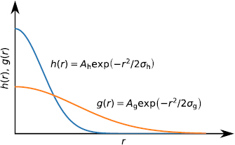
We recall that the assumption of a zero average of the random field was made in the present paper beginning from equation (32). We also emphasize that both specific kinds of functions  and
and  , and their dependence on the coordinates difference, may be different due to uncorrelated noise components along and across the particle velocity (see equations (35)–(37)). As an example, this distinction is illustrated in figure 2 for the simple case when the pair correlation functions
  and
and  decrease with the distance
  according to the Gaussian law but have different values of variance and amplitude. However, it is easy to see that the calculations that lead to the results of the present and subsequent sections of this work do not require the specification of the explicit form of the functions mentioned. We recall that according to equation (4), all restrictions on the general properties of functions R1,2 are contained in the expression

which follows from the Galilean invariance of the system in the absence of external influences. Moreover, since the function R1,2 is a scalar quantity, its dependence on the differences  ,
,  should be characterized by the following expression:

Figure 2. Schematic visualization of a simple example of different behavior of functions  and
and  determining the decrease of pair correlation functions with distance
  according to equation (60).
Download figure:
Standard image High-resolution image
According to equations (59)–(62), equation (55) transforms into
where we introduce
6.1. Brownian particles with active fluctuations. Space-independent noise
Here we study solutions of the kinetic equation (63), which are isotropic in the momentum space.

By taking equations (64) and (65), it is possible to reduce equation (63) to the form
where
The resulting equation (66) is the kinetic equation for active particles with time-dependent nonlinear friction (friction factor  ). This equation can be regarded as a three-dimensional generalization of the kinetic equation for quasi-Brownian particles with active fluctuations, dissipative interaction, and a space-dependent external stochastic field. This fact may be proven if we make some simplifications of equation (66).
First of all, note that the term 'Brownian particles with active fluctuations' is commonly understood as a system of particles under the influence of a space-independent stochastic field given by equations (9) and (10) [3, 21]. Consequently, to prove the above assumption, we should consider the linear friction case in equation (66) and refuse the dependence of the external noise on the coordinates. In the case of linear friction, the friction coefficient  does not depend on the momentum,
  , and, according to equations (5) and (64), the value of
  in this case is given by (see [30]):

However, the consequences of the noise space-independence in equation (66) are rather hard to see immediately. For this we need to repeat the whole procedure of the kinetic equation derivation until equations (55)–(57)—assuming that the values  ,
,  in equation (9) are independent of the coordinates—and conditions (35)–(37) are fulfilled. It turns out that the result of this procedure is equivalent to equating the value
  in equation (66) to zero. Thus, we come to the following equation:
The quantity  is still defined by equations (36) and (60), keeping in mind the fact that the noise characteristic
  does not depend on the coordinate in this case. If in equation (69) we substitute the particles' momentum distribution function f 1(p , t) by the distribution function in the velocity,
  ,
,  , then the equation takes the form usual for the case of quasi-Brownian particles with active fluctuations (see, e.g. [3, 20, 21]). At the same time, the second formula in equation (69) connects the intensity of the 'momentum' noise
  introduced here with the intensity of the 'velocity' noise
  (see equations (9) and (10)). This implies that equation (66) may be regarded as a kinetic equation for quasi-Brownian particles with active fluctuations, which is generalized for the case of a three-dimensional system with dissipative interaction and a nonlocal external stochastic field.
The stationary solution  of equation (69) has a Boltzmann form,

which is different in two-dimensional and three-dimensional cases only by the value of the normalizing constant A (see equation (68)):
Taking into account normalization ((68) and (71)) in the two-dimensional case, the formula (70) for the stationary distribution function of the active particles coincides with the corresponding expression in [3].
6.2. Brownian particles with active local fluctuations
We now investigate the spatially homogeneous stationary states of the system under study in the case of a spatially inhomogeneous external impact. As we already noted (see text explaining formulas (59) and (60), as well as figure 2), spatially correlated noise in certain cases does not prevent the existence of spatially homogeneous states in the system. Let us now consider the stationary solution  of equation (66), which is more general than equation (69). Now equation (66) in the limit
  can be written as follows:

where we introduce

 is given by equation (64), and

defines the nonlinear friction forces. The solution of equation (72) is defined by the relation

The expression similar to equation (75) is given in [18] for the case of two-dimensional active systems with a nonlinear friction coefficient. We emphasize that in this paper, as well as in the general analysis of the above expression, the friction coefficient  is considered to be an arbitrary function of the momentum (in fact, of the velocity
  ,
,  , since the authors of this work performed calculations in the space of velocities not momenta.)
The general analysis of this expression in [18] with an arbitrary dependence of the coefficient of friction on velocity shows that it is the nonlinearity of this coefficient that is one of the necessary conditions for the occurrence of self-propulsion in the system. Indeed, as seen from analysis of the case with nonlinear friction, for one velocity range the dissipation forces may be negative while within the other velocity range the forces may be positive. Thus, the particles with the velocities within the first interval slow down; consequently, this interval corresponds to regular friction. On the contrary, the particles with velocities within the second interval accelerate, that is, they experience propulsion. As a result, a symmetric distribution with two peaks at  is established. We here note that the stationary distribution cannot be isotropic in the velocity (or momentum) space due to the existence of a selected direction
  in the stationary state. Such distribution corresponds to the general solution of the stationary kinetic equation derived in [18] on the basis of the two-dimensional Langevin equation for active particles with a nonlinear friction coefficient. We also note that in [18] the case of the special dependence of the friction coefficient
  on the velocity is analyzed in detail, leading to a linear dependence on the velocity of the friction force itself, but with a shift in the velocity space. It is shown that such a case of linear friction does not prevent the appearance of self-movement in the system. As far as we know, this result was obtained for the first time in the mentioned work. Finally, we note that the special case of linear friction considered in [18] corresponds (both for two-dimensional and three-dimensional systems) to the case
  of linear friction in formula (75) of this work. For more details, see below.
Thus, as will be shown below, it follows from the solution (75) of equation (72) that the stationary distribution function with two maxima (self-propelled particles) can also be realized in the case of linear friction, namely, when  (see equation (68)). This is due to the local impact of stochastic forces with active fluctuations. This leads to the appearance of the factor
  in equation (75), which is defined by the pair correlation functions of the external force and the distribution function itself. This is why the solution of equation (72) is a complex self-consistent task. In fact, the general solution in the case of linear friction, as follows from equation (75), is given by the formula
The display of the head–tail asymmetry is related to the sign of  . Namely, since
  , the positivity of this value,
  , must comply with a purely dissipative case. When
  , there are values of momenta for which the inequality
  is true. Particles moving with the corresponding momentum exhibit self-propulsion. Naturally, the very possibility of the existence of a stationary state presupposes the establishment of a stationary distribution combining both described cases. One of the possible options for achieving such a stationary state in spatially homogeneous systems is the establishment of the regime of two differently directed motions of its structural units with an average momentum p 0 along some selected direction
  . It is this version of the stationary distribution that would correspond to the solution described in [18] for the two-dimensional case. However, the appearance of the selected direction in the momentum space indicates that the stationary state of the system ceases to be isotropic in the momentum space. For this reason, the formal construction of the corresponding stationary distribution on the basis of solution (76) of equation (72) would be incorrect. The reason is that equation (72) was obtained from equation (66) precisely under the assumption of isotropy of the momentum space.
Therefore, in describing the stationary distribution discussed above, it is necessary to start from the most general equation (63). We recall that this equation characterizes the evolution of spatially homogeneous states of the system. In view of the foregoing, the stationary distribution under the steady-state regime of multidirectional movements along one direction should be described by the function

We emphasize that the stationary mode defined by formulas (77)—the possibility of which is predicted by formulas (75) and (76)—is one of the multiple modes possible for the system, not the only one. In this sense, it is one of the particular stationary solutions of the general equation (63) under the assumption (77). An equation for which  holds follows from equation (63) within a limit
  and respects relations (77). It has a form similar to equation (72) if in the latter we assume
  and the absolute values of momentum we replace with
  :
:

For this reason, an analysis of the solutions of this equation can be carried out by analogy of the analysis of formulas (75) and (76) given above (see also [18]). Here, the momentum absolute values are to be replaced by the quantity  , and we assume
  .
.
Thus, taking into account the foregoing considerations for the case of a steady-state regime of multidirectional motions along  , the stationary distribution function of active particles has the form (see [3, 18, 21])
where  is the Heaviside step function, and C is the normalization constant. Momentum p 0 in equation (79), characterizing the location of maxima of the distribution function symmetric with respect to the point p = 0, is determined by
  :
:

The value of  itself, according to equations (73) and (76), depends on the derivative of the unknown momentum distribution function. Thus, the definition (76) with the explicit form of the distribution function (79) should be considered as an equation that connects
  to the normalization constant C:
In turn, the constant C is determined from the normalization condition (see equation (68)
which can be rewritten after combining with equation (79) as
The latter expression is also an equation relating the constant C and the unknown quantity  . Thus, equations (81) and (82) represent a system of two equations to determine two unknown quantities, C and
  , in terms of parameters characterizing the system, namely, the friction coefficient
  , the number density of particles
  , and the parameters of noise with active fluctuations, i.e. the pair correlation function
  and
and  (see equations (73) and (76)). We note that, in contrast to the magnitude of the momentum p 0, the direction
  of steady motion (the self-propelled motion) in the framework of a spatially homogeneous model of a medium with active particles cannot be determined. To determine it, it is necessary to break the spatial isotropy of the system, for example, by introducing anisotropic interaction between particles, even an infinitely small interaction. This will also be mentioned in Conclusion. We also note that because of the integration with respect to the total volume in momentum space, equations (81) and (82) have different forms for two- and three-dimensional cases. Furthermore, the calculation of the integrals over
  in equations (81) and (82) must take into account the anisotropy of the integrands in momentum space. The procedure for calculating these integrals in a spherical coordinate system in momentum space is greatly simplified if the polar axis is assumed to be directed along the vector
  , see (77).
We first consider the two-dimensional case. Equations (81) and (82) take the form
where  is the error integral:

In general, equations (83) are complex transcendental equations that can be solved numerically. However, in the two extreme cases, namely those of small and large values of the argument  of the error integral (84), these equations can be solved analytically. In the case
  , these solutions are given by
With equation (85), the inequality above can be written as

We have already mentioned that the presence of self-propelled properties depends on the sign of  . Since
  is positive (see equation (76)), the quantity
  in equation (85) is negative, i.e.
  . Consequently, a state like a distribution function with two bell-like peaks and parameters defined by equation (85) can be realized.
Now consider the opposite case  . Then, in the main order we get from equation (83):
We see that also in this case the quantity  is negative, i.e.
  , and the particle distribution function is defined by equations (79) and (87). We also add that the inequality
  , can be transformed into the relation

with the use of equation (87). This result is the opposite of equation (86).
Now let us return to equations (81) and (82) and study their solution in the case of a three-dimensional system of active particles with linear friction and active space-dependent (i.e. local in space) fluctuations. In this case, equations (81) and (82) are transformed to a form substantially different from equation (83):
where  is still given by equation (84). As in the previous case of the two-dimensional system of active particles, the second equation in equation (89) in general form can be solved only numerically. However, in the two extreme cases examined above, this equation can be solved analytically. Namely, in the case of small values of the parameter
  the solution of equation (89) is determined by
Furthermore, as is easily seen directly, the ratio  can be reduced to the form equation (86), which is valid for the two-dimensional case.
At large values of the parameter  ,
,  the solution of equation (89) is given by


By analyzing equation (91) we find that at  in the domain of large values of the parameter, the negative
  is only possible if
  . In this case the expression for p 0 can be simplified:

and the condition  can be replaced with an equivalent one,

Thus, we conclude that self-propelled particles can be realized in the case of large values of the parameter  and in the three-dimensional system; however, the criteria (94) in this motion differ significantly from that in the two-dimensional case (see equation (88)).
It should be noted that if  then the characteristic momentum p 0 is always zero, in both two- and three-dimensional cases; see equation (80) and the original equation (72). This should have been expected since this case corresponds to the degeneration of the two bell-like peaks single-particle distribution function into a symmetrical one (with respect to p = 0) of the Gaussian type, with parameters that coincide with those of equations (70) and (71).
It is necessary to emphasize once again that the example we considered in detail above is one of the special cases of the stationary solutions of equation (63). It is clear that the stationary states of the system, which satisfy the stationary variant of equation (63), can also have a more complex form while remaining spatially homogeneous. We have chosen this type of solution (see (76)–(94)) precisely because it reproduces formulas that demonstrate the self-propelled properties of the systems under consideration, which are similar to the self-propelled results, for example, of [3, 18, 21]. It should be noted here that the self-propulsion in active media in this paper is described as a collective effect and a consequence of the influence of spatially correlated noise. But at the same time, for the manifestation of the self-propulsion effect in the system, the particles (even if they are considered to be points) should have the property of head–tail asymmetry. That is, one of the reasons for the possible manifestation of the properties of the self-propelled system are the individual characteristics of the particles—the structural units of the system. In our model, this was ensured by the dependence of the influence of noise on the magnitude and direction of the velocity of the particle itself. Thus, with the external similarity of the results of the present work and, for example, the work [18], the reasons leading to these results may be different. Recall that in [18] one particle is considered, which is logical for an approach that uses the Langevin equations as the initial equations for the individual motion of particles. The driving force arising in such a system is not a collective effect. However, it should still be borne in mind that a phenomenological approach was used in [18], where a nonlinear friction force in the medium was assumed, and a very specific dependence of the friction coefficient on speed was postulated.
In concluding this section, it is necessary to reiterate the following. In a number of places above, we specifically separated the cases of two-dimensional and three-dimensional systems. From the procedure for constructing the kinetic theory of active media in the microscopic approach described in the paper, it can be seen that there is no conceptual difference between the derivation of equations in two- and three-dimensional cases. However, the situation looks this way only after the equations of motion (6)–(9) are written out. These equations are formulated to replace the two-dimensional Langevin equations, which usually underlie the construction of the kinetic theory of active media. The generalization of the initial equations of motion for structural units, as could be seen, is completely nontrivial. In fact, as was noted in Introduction, historically, when constructing the kinetic theory of active media, authors, as a rule, proceeded from the two-dimensional Langevin type equation (10). In some cases, the interactions between the structural units of the system were included in the aforementioned Langevin equations; see, for example, [1–6, 19–21]. However, building a consistent microscopic approach to deriving the kinetic equations of such media requires going beyond the scope of the Langevin equations as the initial equations of motion for the structural units of the system. Instead of the Langevin equations, it is necessary to formulate the generalized Hamilton equations, that is, to start from the first principles of classical theoretical mechanics. For this reason, in this paper we proceeded from the generalized Hamilton equations, which naturally allow us to include both interactions between particles (including dissipative interactions) and a three-dimensional view of the stochastic effect on the system, depending on the speed and coordinates of structural units. Furthermore, in order to compare the results that follow from our theory in certain particular cases with the results of other authors (for two-dimensional systems), we separated in some cases the results for three-dimensional and two-dimensional systems. It should also be noted that in the framework of the model we are considering, the conditions (or criteria) for the existence of self-propulsion in the system may differ for two-dimensional and three-dimensional systems (see, for example, (88) and (94)). At the same time, the very possibility of the existence of such self-propulsion modes in both two-dimensional and three-dimensional cases is not prohibited.
7. Conclusion
In this paper we propose a microscopic approach to construct a kinetic theory of many-particle systems with dissipative and potential interactions in the presence of active fluctuations. The approach is based on a generalization of the Bogolyubov–Peletminskii reduced description method applied to the systems of many active particles. The microscopic approach allows us to construct the kinetic theory of active particles in the case of two-dimensional and three-dimensional systems, as well as in the presence of a nonlinear friction and local active fluctuations. We obtain general kinetic equations for these systems in the case of a weak interaction between the particles (both potential and dissipative) and low-intensity active fluctuations. We define some particular cases in which the derived kinetic equations have solutions that match with the results for the systems of active particles known from earlier works by other authors. It is also shown that one of the consequences of the local nature of the active fluctuations is a manifestation of a head–tail asymmetry and a self-propulsion, which is typical for systems of active particles, even in the case of a linear friction (see equations (83)–(94)).
We recall that in this context formulas (83)–(94) describe only two special limiting cases of two-dimensional and three-dimensional systems with self-propelled particles. The expressions obtained for a two-dimensional case coincide with those derived in [3, 21]. However, in our approach the nature of the phenomenon of self-propulsion is associated with a local (individual) exposure to the particles of the external stochastic field with active fluctuations, see equation (9). Besides, the parameters of the self-propelled motion are self-consistently expressed by the internal characteristics of a many-body system, namely the number density of particles in the system, the parameters of the dissipative function, and the characteristics of the external influence, that is, the pair correlation function of the active random field. Note that the stationary direction of the head–tail asymmetry within the spatially homogeneous model (see equations (65) and (66)) cannot be determined. To define it, we should introduce an interaction, even an arbitrarily small one; however, this violates the spatial isotropy of the problem. In this sense, the situation expressed by equations (79)–(88) is similar to the situation with a phase transition to the magnetic ordering in ferromagnets, see, e.g. [42]. As is known, the value of the total magnetic momentum in a ferromagnet in the main approximation is determined by the isotropic exchange interaction. The direction of the magnetization is at the same time given by nonisotropic weak relativistic interactions. The situation with the appearance of anisotropy in the momentum space as a result of a phase transition in a normal Fermi-liquid with a weakly anisotropic interaction was also considered in [43].
Here we note that the kinetic equations (55)–(57) are general in the sense that they describe quite a number of different many-particle systems, both two-dimensional and three-dimensional ones, with active local fluctuations, homogeneous and inhomogeneous space, and different variations in the nonlinear friction. The study of various particular cases of solutions of kinetic equations (55)–(57) is beyond the scope of this paper. As outlined above, the main objective of this work is the development of a microscopic approach to derive the general kinetic equations for active particles with nonlinear friction under the influence of active fluctuations, including a generalization to the case of three-dimensional systems.
We also note that the microscopic approach suggested here for the construction of the kinetic theory of many-particle systems with dissipative interaction and active fluctuations allows for further generalization, e.g. to the case of simultaneous presence of both active and passive fluctuations. Furthermore, a nonGaussian stochastic nature of external effects can be taken into account; see also in this regard [18].
Acknowledgments
The authors would like to thank Prof A Chechkin for fruitful discussions and valuable comments on the paper.
OS acknowledges the support by the Spanish Ministry of Economy and Competitiveness MINECO through BCAM Severo Ochoa excellence accreditation SEV-2013-0323 and SEV-2017-0718.