
Abstract
We consider a system of hard spheres with gravitational interactions in a stationary state described in terms of the microcanonical ensemble. We introduce a set of similar auxiliary systems with increasing sizes and numbers of particles. The masses and radii of the hard spheres of the auxiliary systems are rescaled in such a way that the usual extensive properties are maintained despite the long-range nature of the gravitational interactions, while the mass density and packing fractions are kept fixed. We show, within that scaling limit, that a local thermalization spontaneously emerges as a consequence of both extensive properties and the relative smallness of the fluctuations. The resulting mass density profile for the infinite system can be determined within a hydrostatic approach, where the gradient of the local hard-sphere pressure is balanced by the average gravitational field. The derivation sheds light on the mechanisms which ensure that the local equilibrium in the infinite system is entirely controlled by hard-core interactions, while gravitational interactions can be treated at the mean-field level. This allows us to determine the conditions under which the hydrostatic approach is also valid for the actual finite system of interest. We provide simple tests of such conditions for a few astrophysical examples.
Export citation and abstract BibTeX RIS
1. Introduction
For a long time in astrophysics, the equilibrium states of systems made up of objects with gravitational interactions have been studied within a hydrostatic framework [1]. A local thermodynamical equilibrium is assumed while the global structure of the system is determined by balancing the pressure force associated with spatial inhomogeneities and the gravitational force induced by the whole mass distribution. The simplest version of that approach, known as the model of the isothermal sphere [2, 3], is obtained by using the local pressure of an ideal gas. This mean-field theory is analogous to that introduced by [4] for studying the internal structure of a star. Other more sophisticated versions, using in particular a local pressure which accounts for short-range interactions, have also been introduced. The hydrostatic approach has been widely applied to many astrophysical objects like globular clusters, for instance (see [5] for a review).
Beyond the hydrostatic approach, statistical mechanics descriptions of gravitating systems with N particles have been introduced further [6]. In particular, for various models and statistical ensembles [7, 8], it has been proved that the hydrostatic approach emerges within appropriate scaling limits (SLs), where the gravitational coupling is rescaled with N and vanishes in the limit N → ∞. Fluctuations of the total gravitational field can be neglected, as suggested first by [9]. However, we stress that this does not mean that the hydrostatic approach is valid for a given finite self-gravitating system, where all physical parameters, and in particular the universal gravitational constant, are given once and for all. In fact, some drawbacks of hydrostatic approaches like Antonov's mean-field theory have already been quoted, but a systematic analysis within statistical mechanics has never been carried out, to our knowledge. That question is of central importance, as far as astrophysical applications are concerned.
The aim of this paper is precisely to derive a simple statistical mechanics framework for analysing the reliability of the hydrostatic approach applied to a given self-gravitating astrophysical system. For that purpose, we first introduce a rather realistic model, namely a system  made up of N identical hard spheres with two-body gravitational interactions and enclosed in a spherical box. Collisions among the particles are elastic and, therefore, no aggregation phenomenon takes place. Particles also collide elastically with the walls of the confining box. We consider a stationary state described by the microcanonical distribution. All microcanonical quantities are finite, thanks to the presence of hard cores which prevent the divergences3 observed for point particles with N ⩾ 3 [12].
The stationary state of  depends on three dimensionless parameters: the energy ε in units of a typical total gravitational energy, the hard-sphere packing fraction η, and the number of particles N. Since N will be large in astrophysical applications, it is convenient to construct a limit reference system
  with the same values of the parameters ε and η. This can be achieved through a limit process inspired from the usual thermodynamic limit (TL), namely a sequence of larger and larger auxiliary hard-sphere gravitating systems
  with increasing particle numbers Na and the same values of ε and η. In order to ensure that the intrinsic quantities of
  only depend on ε and η, it is crucial to maintain the extensive properties, which would break down in the usual TL because of the long-range nature of the gravitational interaction. Thus, we are left to introduce masses ma and hard-sphere diameters σa which depend on Na. Within the extensivity requirement and the constraints εa = ε and ηa = η, it turns out that particles become smaller and lighter as Na increases. Interestingly, in that SL, the mass density of
  is kept fixed, as well as the internal mass density of the hard spheres. That SL turns out to be a natural extension of the familiar TL where the particle density is kept fixed.
Once the SL has been defined, we study the mass density profile of  by investigating the asymptotic behaviour of its microcanonical expression for
  . Our analysis relies on simple estimations based on our scaling, and additional plausible assumptions concerning fluctuations which are checked a posteriori. We derive a Boltzmann-like formula for the inhomogeneous density in terms of the mean-field gravitational potential created by the whole mass distribution, where the average kinetic energy per particle plays the role of the temperature. This allows us to infer that a local thermodynamical equilibrium entirely controlled by hard-core interactions arises, while gravitational interactions can be treated at the mean-field level. The resulting mass density profile of
  is determined by the hydrostatic equation which expresses the balance between the gradient of hard-sphere pressure and gravitational attraction. This is in agreement with the picture of
  as a continuous medium which emerges from the SL, where particles become points while their number in any given finite volume diverges. The a priori assumptions on fluctuations are shown to be satisfied, thanks to the large separation between the local correlation length on the one hand, and the typical density-variation length associated with gravitational interactions on the other hand. Although our derivations are not mathematically rigorous, the results obtained should be exact, at least at not too low values of ε for a given η.
With the introduction of the sequence of auxiliaries system  , we can answer the central question of this paper, which concerns the reliability of the hydrostatic approach for describing the actual system
  of interest. First, our derivations shed light on the mechanisms which lead to the hydrostatic equation for the infinite system
  defined through the limit of the sequence
  . In that limit process, the role of extensivity turns out to be crucial for the emergence of a local temperature uniform in the whole system. We stress that the relative smallness of the macroscopic fluctuations is another essential ingredient. Second, the corresponding analysis provides a set of simple necessary conditions for the parameters (ε, η, N) which guarantee the validity of the hydrostatic approach for
  , which is the first element of the sequence
  . Other scalings leading to the hydrostatic approach could have been introduced, but we stress that they would not affect the previous validity conditions for the finite system.
The paper is organized as follows. In section 2, we introduce the model as well as our scaling continuous limit. The scaling properties of the potential energy and of the mass distribution are described in section 3, followed by a heuristic introduction of a simple ansatz for the fluctuations of the potential energy. In section 4, we derive a Boltzmann-like formula for the inhomogeneous density, from which we infer the emergence of a local thermodynamical equilibrium. This allows us to introduce the hydrostatic approach, as discussed in section 5. In section 6, we derive a set of necessary conditions which ensure the validity of the hydrostatic approach for the finite system  of interest, and we test them in a few astrophysical examples. Eventually, our main results are summarized in section 7. We also provide additional comments about the reliability of the hard-sphere model and of its microcanonical description with a view to practical applications. In particular, dynamical issues concerning relaxation towards equilibrium are briefly mentioned.
2. Definitions
2.1. The system  in the microcanonical ensemble

We consider a classical gravitational system  , made up of N identical hard spheres with mass m and diameter σ, enclosed in a spherical box of volume Λ = 4πR3/3. The corresponding Hamiltonian reads

with the two-body interaction potential

We consider that the previous system is isolated and does not exchange energy with some thermostat. Thus, its energy is fixed and equal to some value E. We assume that the corresponding stationary state is described within the microcanonical ensemble. The corresponding distribution of positions and momenta of the N particles in the canonical phase space reads

while the total number of microstates is

where AN is some normalization constant, which is not relevant for our purpose.
The microcanonical distribution fmicro remains stationary under the time evolution generated by Hamiltonian HN. We stress that Ω(E, N, Λ) is finite for σ > 0, while it diverges for point particles with σ = 0 for N ⩾ 3 as shown in [12]. The corresponding stationary state of total mass M = Nm is controlled by three independent dimensionless parameters, namely N, ε (which is the energy in units of GM2/R), and the packing fraction η = πnσ3/6 with the particle density n = N/Λ. Notice that ε is identical to the parameter which entirely controls the stationary state of a system composed of point particles within Antonov's mean-field theory [2].
2.2. The scaling continuous limit for the auxiliary systems

Since we are interested in the properties of a system with a large number of particles, it is useful to consider a sequence of larger and larger auxiliary hard-sphere gravitating systems  with increasing particle numbers Na and take some limit where Na → ∞. For ordinary systems with short-range interactions, that limit is nothing but the usual thermodynamic limit where both the energy per particle Ea/Na and the particle density na = Na/Λa are kept fixed. In that limit, the physical parameters which describe a given particle are also kept fixed. Because of both the attractive and the long-range natures of the gravitational interaction, such a limit would provide a collapsed state with non-extensive properties. In order to describe other physical situations of interest, other limits have been introduced in the literature, like the one describing an infinitely diluted system [14].
Here, we want to build a SL when Na → ∞, which describes an infinite continuous fluid  with the usual extensive properties and depending only on the parameters ε and η characterizing the actual system of interest
  . For that purpose, we consider that the parameters which define the particles of
  vary with Na like power laws, while the gravitational constant G is not rescaled, in contrast to the case for some mean-field scalings introduced in the literature [7, 8]. Therefore, we set σa = (Na/N)ασ and ma = (Na/N)δm, while the size Ra of the spherical box is chosen to diverge as (Na/N)γR with γ > 0 so that the system does indeed become infinitely extended. The particle density na = Na/Λa behaves then as
  . By imposing that
  remains constant and equal to η, we find a first constraint

Since Ea is chosen extensive, while  with Ma = Nama is kept fixed, the gravitational energy
  also has to be extensive. This implies the second constraint

At this stage, we have the two constraints (5) and (6) for three exponents, so we can impose a third constraint. By analogy with the usual TL where the number density is fixed, we impose here that the mass density ρa = mana remains constant and equal to ρ, which leads to

The three exponents are then readily determined as α = −2/15, δ = −2/5 and γ = 1/5. Thus, the power laws defining the required SL when Na → ∞ are

As illustrated in figure 1, that limit clearly describes an infinite continuous medium  , the state of which is controlled by the two independent parameters ε and η. Note that, within the scaling considered, the mean free path
  remains proportional to the diameter σa of the hard spheres,
  . Therefore, for high dilutions such that η ≪ 1, ℓa is much larger than σa.
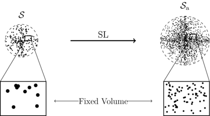
Figure 1. Particles become infinitely small and light in the SL, while their inner mass density  remains constant. Their number density na diverges as
  , while the mass density ρa is indeed kept fixed and equal to ρ, as well as the packing fraction ηa = η and the dimensionless energy εa = ε.
Download figure:
Standard image High-resolution image3. Scaling properties of the auxiliary systems
3.1. H-stability and extensivity of the potential energy
For any allowed configuration, the potential energy of the system  ,
,

is larger than that of the collapsed configuration where the Na hard spheres make a single cluster with size  , which is of order
  . In the SL, the collapse radius Lcoll diverges as
  and this provides the classical version of H-stability [13]:

where CHS is a positive real number entirely determined by the geometrical arrangement of the hard spheres at maximum packing. On the other hand, the potential energy should reach its maximum when all particles are homogeneously distributed on the spherical surface of the box. That maximum behaves as the gravitational energy of an empty sphere carrying the surface mass density  , so we expect the upper bound

According to bounds (10) and (11),  remains of order Na for any configuration. This implies extensive lower and upper bounds for the average potential energy
  , where 〈A〉 denotes the microcanonical average of any observable A weighted by the microcanonical distribution for system
  , namely expression (3) with (N, AN, HN, E) replaced by
  . Therefore, the non-extensive behaviour of the average potential energy encountered in the usual thermodynamic limit does not occur in the present SL. Accordingly, the extensivity of
  should be ensured here. Since the typical potential energy
  is also extensive by construction of the SL, we find

where u(ε, η) is the dimensionless potential energy per particle of the infinite system  , which only depends on the intensive dimensionless parameters ε and η.
3.2. Mass distributions
For further purposes, it is useful to introduce the n-body mass distributions. Let us consider first the one-body mass distribution, which reads

According to the scaling properties of the potential energy described above, we can reasonably expect ρa(r) to take a well-defined shape in the SL, which is the mass distribution ρ∞(r) of the infinite system  . Taking into account dimensional and spherical-symmetry properties, this leads to

where q = r/Ra remains fixed in the SL. The function g(q; ε, η) is the dimensionless mass distribution, as a function of the rescaled distance q, for the equilibrium state of  determined by the intensive parameters (ε, η). The two-body mass distribution is
while similar definitions hold for higher order n-body mass distributions with n ⩾ 3. The scaling property (14) can be extended to such mass distributions, namely

and so on.
We can check that the expected extensive behaviour of the average potential energy of  is consistent with the above scaling properties for the mass distributions. This is easily seen by starting from the integral expression

After making the change of variables r → Rq, r' → Rq', and using the scaling behaviour (16) for  , we find that
  is indeed an extensive quantity in the SL.
3.3. Fluctuations of the potential energy
Let us now consider the fluctuations of the potential energy around its average. Such fluctuations can be rewritten, similarly to formula (17), as

where  and
and  are the three- and four-body mass distributions. In the SL, the first two terms in expression (18) can be estimated by replacing
  and
and  by their scaling behaviours in terms of g(2)(q, q'; ε, η) and g(3)(q, q', q''; ε, η). The first term is then found to be of order
  , while the second one behaves as Na.
If we estimate the third term in expression (18) by using only the scaling behaviours of the mass distributions involved, we obtain not surprisingly an  -behaviour. However such an estimation should overestimate the exact behaviour, because the correlations involved

can reasonably be expected to become rather small compared to ρ4, for spatial configurations (r, r', r'', r''') describing a large part of the integration domain  . A precise estimation cannot be performed at this level, so here we only assume that the third term in expression (18) should grow slower than
  .
.
The previous simple arguments suggest that the square of fluctuations (18) should become small compared to  in the SL, i.e.

Note that the corresponding fluctuations for an ordinary system with short-range interactions at thermodynamical equilibrium do satisfy the behaviour (20) since they are proportional to Na.
3.4. The scaling decomposition ansatz
In the following, we will have to take averages of quantities involving the potential energy  . Taking into account the extensivity of its average, as well as the behaviour (20) of its fluctuations, we propose to decompose
  as
as

with  and
and  in the SL. We assume that such a decomposition ansatz holds for most probable configurations, which mainly determine the averages of interest, so it should provide the exact behaviours in the cases studied further.
Note that both the extensivity of  and the fluctuation behaviour (20), although quite plausible, are not rigorously proved from a mathematical point of view. In fact, we will show a posteriori that the mass distributions and correlations inferred from the decomposition ansatz are such that the a priori assumptions about
  and
and ![$(\langle V_{N_{\rm a}}^2 \rangle - [\langle V_{N_{\rm a}} \rangle ]^2)$](https://content.cld.iop.org/journals/1751-8121/47/22/225001/revision1/jpa494779ieqn66.gif) are indeed satisfied. This provides some kind of consistency check of the derivations.
are indeed satisfied. This provides some kind of consistency check of the derivations.
4. Emergence of local thermalization in the SL limit
In this section, we consider the inhomogeneous mass density ρa(r) given by average (13), and we study its asymptotic behaviour in the SL. First, we express ρa(r) in terms of the gravitational potential created by all of the particles except one, which is fixed at position r. Then, by combining the extensivity of the potential energy together with the decomposition ansatz (21), we show that the SL expression for ρa(r) takes the form of a Boltzmann-like formula. The corresponding temperature is merely related to the average kinetic energy per particle of  , which is indeed an intensive parameter in the SL. We briefly show that similar formulae hold for the one-body distribution
  in phase space, as well as for higher order mass distributions.
4.1. Introduction of the gravitational potential
As a starting point, we compute the average (13) with the microcanonical distribution for  . Then, the standard integration over the momenta of the Na particles leads to

In that expression, θ(ξ) is the usual Heaviside function such that θ(ξ) = 1 for ξ > 0 and θ(ξ) = 0 for ξ < 0, while the normalization constant B(Ea, Na, Λa) ensures that the spatial integral of ρa(r) over the box does provide the total mass Ma of the system. The conditions |ri − rj| > σa, arising from the hard-sphere interaction, apply to any pair of particles, and in particular those including particle 1 fixed at r1 = r.
For ε > −1/2, it turns out that  is positive for any spatial configuration thanks to the upper bound (11) for the potential energy. Then, the Heaviside function can be exactly replaced by 1 in the expression (22). For ε ⩽ −1/2, there are spatial configurations which are forbidden. However, in the SL, the average of the kinetic energy
  is necessarily strictly positive and extensive. Thus, for the most probable configurations which provide relatively small fluctuations as a consequence of the decomposition ansatz (21), that quantity is still positive. Thus, it is legitimate to discard the condition
  in the SL for any value of ε, except that corresponding to the collapse into a single ball of course.
The previous simplification is crucial for further transformations. In particular, let us introduce the gravitational potential  at r created by the (Na − 1) particles located at
  . According to the decomposition

we can rewrite formula (22) in the SL as

where  denotes the unnormalized microcanonical measure for the spatial configurations
  of a system made up of (Na − 1) particles, enclosed in the same spherical box with volume Λa and the same energy Ea as the system
  with Na particles,

4.2. Exploiting the extensivity of the potential energy
Let us consider the identity

Since  and
and  , we can expand the logarithm in powers of
  . After multiplication by the factor (3Na/2 − 1), we see that the linear term provides a contribution of order
  , while higher powers provide vanishing contributions when Na → ∞. Accordingly, we obtain for any spatial configuration

in the SL. Inserting that asymptotic behaviour inside the rhs of formula (24), we infer the SL behaviour

We stress that the extensivity of the potential energy for any spatial configuration, which follows from the particular scaling defined here, plays a crucial role in the derivation of the asymptotic expression (28). Within other scalings, which do not preserve that remarkable extensivity property, the asymptotic behaviour (28) would break down.
4.3. A Boltzmann-like formula for the mass distribution
If we introduce the kinetic energy  of the (Na − 1) particles for a given spatial configuration, the exponential factor on the r.h.s. of the asymptotic expression (28) can be seen as some kind of Boltzmann factor. However, at this level, the corresponding temperature fluctuates. Here, we show that such fluctuations can be neglected on applying the fluctuation ansatz described in section 3.
The integral with the measure  in the rhs of formula (28) is proportional to the microcanonical average of the quantity

for the system with (Na − 1) particles. For estimating that average in the SL, we can apply to  the decomposition ansatz (21) with Na → (Na − 1). The resulting contribution of fluctuations
  can be omitted at leading order. Moreover, since the corresponding average of
  differs from
  by a term of order
  in the SL, all factors
  can be replaced by
  at leading order.
Similarly to the potential energy  , the gravitational potential energy
  can be reasonably expected to display small relative fluctuations around its average, which is of order
  in the SL. Apart from terms of order o(1), that average reduces to the mean gravitational potential

created by the whole mass distribution ρa(r'). Therefore, in the above average of quantity (29), we can replace  by maϕa(r) at leading order in the SL.
Since all contributions from fluctuations of both  and
and  can be neglected at leading order, we eventually recast the asymptotic behaviour (28) as

where the microcanonical temperature T(Ea, Na, Λa) is defined through the usual relation

while C(1)(Ea, Na, Λa) is a normalization constant.
4.4. Identification of a local thermodynamical equilibrium
According to formula (31), the particle fixed at r interacts with the other particles only via hard-core interactions, while the average gravitational potential plays the role of an external potential Vext(r) = limSLmaϕa(r). On the other hand, the occurrence of the Boltzmann factor exp ( − maϕa(r)/T(Ea, Na, Λa)) shows that a local thermodynamical equilibrium takes place at temperature T(Ea, Na, Λa). Hence, a local equilibrium in  emerges, and it is identical to that of thermalized pure hard spheres subjected to an external potential Vext(r) = limSLmaϕa(r). That picture is confirmed by the calculation of the one-body distribution
  , which behaves in the SL as

while the n-body mass and phase-space distributions are given by simple extensions of formulae (31), (33).
The previous identification of a local thermodynamical equilibrium constitutes the central observation which will allow us to introduce the hydrostatic approach for studying the properties of  , as described in the next section. Notice that the temperature defined through relation (32) remains intensive in the SL, and it reduces to some temperature T∞ for the infinite system
  , where the rescaled dimensionless temperature T∞/(GM2/NR) is a function T*(ε, η) of the intensive parameters ε and η.
5. The hydrostatic approach for the infinite system
In this section, we will show that the mass distribution of  can be determined by applying the hydrostatic approach. For that purpose, we proceed to various estimations, which rely on the local structure of the auxiliary systems
  in the SL limit Na → ∞, inferred in the previous section. We conclude through similar estimations for the contributions of correlations and fluctuations, which justify a posteriori our whole scheme.
5.1. Separation of scales and the hydrostatic balance
In the SL limit, the local equilibrium in  is entirely determined by the local packing fraction ηa(r) = ηρa(r)/ρ. In particular, the decay of particle correlations is controlled by the local hard-sphere correlation length [15, 16]

where ξHS(η) is some dimensionless function of η. Let us assume a priori that the system remains in a fluid phase at the local level, i.e. the local packing fraction does not exceed some critical value ηLC, for which the system is expected to undergo a phase transition from a liquid to a crystalline phase [15, 16]. Then ξHS(ηa(r)) remains bounded everywhere, so λa(r) behaves as σa and vanishes as  in the SL.
Since the mass density ρa(r) is expected to vary on a length scale of order Ra, Vext(r) also varies on distances of order Ra. Thus, the external potential seen by the hard spheres is almost constant over their local correlation length λa(r). The corresponding density profile is then easily obtained through a straightforward application of density functional theory [17, 18], where the free energy functional can be merely replaced at leading order by its purely local expression built with the free energy density of a homogeneous system. Corrections due to spatial inhomogeneities of the density profile can be safely neglected here because they are of order  in the SL, as estimated from a systematic expansion in powers of the density gradient [19–22]. The familiar hydrostatic equation for the density profile in the external potential Vext(r) = maϕa(r) then follows on taking the gradient of the variational equation associated with the local functional. The local pressure comes out when differentiating the local free energy density and it reduces to that of a homogeneous gas of pure hard spheres without gravitational interactions, at temperature T and number density ρa(r)/ma, i.e.

where pHS is the dimensionless hard-sphere pressure which depends only on the local packing fraction ηa(r) = ηρa(r)/ρ.
According to the previous infinite separation of typical lengths in the SL limit, the mass density profile and the corresponding gravitational potential for the infinite system  are exactly determined within the hydrostatic approach. The corresponding coupled equations can be recast for the dimensionless rescaled quantities g(q; ε, η) = limSLρa(Raq)/ρ and ψ(q; ε, η) = limSLϕa(Raq)/(GMa/Ra) of
  , as
, as

and

Those equations have to be solved inside the unity sphere together with the rescaled-mass constraint

and the rescaled-energy constraint

We recall that the dimensionless temperature T*(ε, η) has to be determined through the resolution of the whole system of equations, where ε and η are the fixed control parameters.
The properties of the coupled equations (36), (37) have been widely studied in the literature. Once the SL has been taken, the limit of point particles corresponding to η = 0 is now well-behaved, and it is readily obtained by replacing the hard-sphere pressure by its ideal counterpart, namely by setting pHS(ηg(q; ε, η)) = 1 in the dimensionless hydrostatic equation (36). We then recover Antonov's mean-field theory, for which analytical results are available [2, 24]. For η ≠ 0, various numerical studies have been performed by using approximate simple forms of the hard-sphere equation of state pHS(η) [25, 26].
Eventually, let us quote that the system does not remain in a fluid phase everywhere if ε becomes too close to the collapse lower bound εcol(η) related to the minimum (10) of the potential energy. The core region then undergoes crystallization4, so the hydrostatic equation should be replaced by some elasticity equation incorporating the stress induced by the gravitational field. Moreover, use of the hydrostatic approach for describing the interface with the fluid region outside the solid core would be rather questionable. Notice that close to the wall of the spherical box, i.e. for r almost equal to Ra, the mass density ρa(r) varies on a scale σa, so the hydrostatic approach fails in that region. Indeed, use of a purely local functional for the free energy is no longer valid and would lead to a violation of the contact theorem (see e.g. ref. [23]). This does not affect the shape of ρa(qRa) in the SL for fixed q < 1.
5.2. Correlations and fluctuations
The derivations in section 4, which ultimately lead to the hydrostatic equations, involve a priori assumptions about the relative smallness of fluctuations. Here we estimate the contributions of such fluctuations, based on simple modellizations of correlations which follow from the local structure of  in the SL limit.
First, we can estimate the contributions of correlations to the average gravitational energy which, according to formula (17), can be recast as

In that decomposition, Vself is the self-gravitational energy of a sphere with mass density ρa(r),

while Vcorr is the correlation energy

with the truncated mass distribution or mass correlations,

In the SL, Vself behaves extensively, and it is determined at leading order by the solutions of the hydrostatic equations for  . Taking into account the local structure of
  , we find that
  reduces to −ρa(r)ρa(r') for |r − r'| < σa. Moreover, we expect
  to vanish over the hard-sphere local correlation length λa(r). As argued above, λa(Raq) becomes proportional to σa in the SL. Thus, the contribution of the vicinity of point r = Raq to

is of order  in the SL. The remaining contribution to the integral (44) of points r' such that |r − r'| ≫ σa can be roughly estimated by replacing
  by a constant times maρa(r)/Λa which does not depend on r'. That spread homogeneous approximation is inspired by the sum rule

which follows from particle conservation. The corresponding contribution to integral (44) is then of order  which becomes small compared to that of the region |r − r'| ∼ σa. Accordingly, we find that the correlation energy (42) is of order
  . Thus,
  is indeed extensive, and the rescaled potential energy per particle (12) is entirely given by the self-part Vself, namely

Let us consider now the fluctuations ![$(\langle V_{N_{\rm a}}^2 \rangle - [\langle V_{N_{\rm a}} \rangle ]^2)$](https://content.cld.iop.org/journals/1751-8121/47/22/225001/revision1/jpa494779ieqn118.gif) of the potential energy, which are given by formula (18). We can rewrite the first two terms as mean-field-like terms
of the potential energy, which are given by formula (18). We can rewrite the first two terms as mean-field-like terms

and

plus the corresponding correlation terms associated with ![$[\rho _{\rm a}^{(2)}(\mathbf {r},\mathbf {r}^{\prime })-\rho _{\rm a}(\mathbf {r})\rho _{\rm a}(\mathbf {r}^{\prime })]$](https://content.cld.iop.org/journals/1751-8121/47/22/225001/revision1/jpa494779ieqn119.gif) and
and ![$[\rho _{\rm a}^{(3)}(\mathbf {r},\mathbf {r}^{\prime },\mathbf {r}^{\prime \prime })-\rho _{\rm a}(\mathbf {r})\rho _{\rm a}(\mathbf {r}^{\prime })\rho _{\rm a}(\mathbf {r}^{\prime \prime })]$](https://content.cld.iop.org/journals/1751-8121/47/22/225001/revision1/jpa494779ieqn120.gif) . Since ρa(r) does satisfy the scaling property (14) in the SL, the mean-field contributions (47) and (48) are of order
. Since ρa(r) does satisfy the scaling property (14) in the SL, the mean-field contributions (47) and (48) are of order  and Na respectively. The corresponding two- and three-body correlation contributions are readily estimated within a simple modellization of the truncated distributions analogous to the one used above for analysing contribution (42) to the average
  itself. They are found to become small compared to their mean-field counterparts in the SL.
It remains to estimate the contribution of the third term in expression (18) of the fluctuations ![$(\langle V_{N_{\rm a}}^2 \rangle - [\langle V_{N_{\rm a}} \rangle ]^2)$](https://content.cld.iop.org/journals/1751-8121/47/22/225001/revision1/jpa494779ieqn123.gif) . If we define
. If we define

we can rewrite that four-body correlation term as

Like for the case of  , we expect, for two given points r and r',
  to take finite values of order ρ2 for spatial configurations such that one or more of the relative distances |r'' − r|, |r'' − r'|, |r''' − r'|, |r''' − r''| is of order σa. The corresponding contributions to the integral

are then readily estimated along lines similar to the above when analysing the two-body correlation term (44). For each of the four regions where one of the points r'' or r''' is close to either r or r', we find a contribution to integral (51) of order  . After integration over r and r', the corresponding contribution to the term (50) is
  . All the other spatial configurations (r'', r''') for which hard-sphere correlations determine
  , ultimately provide contributions o(Na) to (50). Eventually, it remains to determine the contributions of regions such that all distances |r'' − r|, |r'' − r'|, |r''' − r'|, |r''' − r''| are large compared to σa. As for the case of
  , we again use a spread homogeneous approximation inspired by the sum rule

namely, we replace  by a constant proportional to
  . This provides a contribution of order 1 to integral (51), and ultimately a contribution
  to (50). Accordingly, the four-body correlation term (50) is of order Na, so fluctuations
 ![$(\langle V_{N_{\rm a}}^2 \rangle - [\langle V_{N_{\rm a}} \rangle ]^2)$](https://content.cld.iop.org/journals/1751-8121/47/22/225001/revision1/jpa494779ieqn133.gif) do indeed grow more slowly than
do indeed grow more slowly than  , in agreement with the assumption (20).
The previous estimations confirm that gravitational interactions can be treated at the mean-field level in the SL limit. In particular, the gravitational energy is indeed dominated by the mean-field self-term (41), as assumed in variational derivations of the hydrostatic equations [2]. Furthermore, fluctuations of that gravitational energy can be discarded. This constitutes a consistency check a posteriori for our derivation of the hydrostatic approach.
6. Validity conditions for the finite system

If the hydrostatic approach is legitimate for studying the infinite system  , this does not mean that it provides an accurate description of the finite system
  of interest. In fact, the derivation of section 4 relies on various estimations for the auxiliary systems
  which are asymptotically valid in the limit Na → ∞. When considering
  , where the number of particles Na = N is finite, such estimations may break down. Thus, their validity for
  implies various necessary conditions for the dimensionless parameters (N, ε, η).
6.1. The introduction of Boltzmann-like exponentials
The exponentiation formula (27) plays a crucial role in the further emergence of Boltzmann factors. That asymptotic formula works in the SL thanks to extensivity properties of systems  . For the finite system
  , its validity requires

That condition has to be fulfilled by the most probable configurations which determine the equilibrium state of  . If we assume a priori that the hydrostatic approach is accurate for
  , the gravitational potential and gravitational energy involved in condition (53) can be replaced by their average values determined by the rescaled solutions of the hydrostatic equations (36), (37), namely

and

In the replacement (54), we have set r = 0 because |ϕ(r)| is maximum at r = 0, so the condition (53) will indeed be fulfilled for any r. According to the above replacements, that condition can be recast as

Not surprisingly, for given values of ε and η, this means that the number of particles N of  must be large enough. For a given value of N, the temperature T*(ε, η) has to be large enough, or in other words the mean kinetic energy has to be large enough.
6.2. Omission of fluctuations
Another crucial step in the introduction of Boltzmann factors associated with the average gravitational potential relies on the estimation of the a priori fluctuating exponential

Fluctuations can be omitted if the corresponding variations of the exponent

are small compared to 1. A typical fluctuation of ΦN − 1(r) can be readily estimated by considering the fluctuations of position of one particle j with j > 1 close to the particle fixed at r1 = r. On average, the corresponding relative distance |rj − r1| is of order a = (3/4πn)1/3, while that distance becomes σ when the two particles are in contact. The resulting variation of mΦN − 1(r) is of order

In the corresponding variation of the exponent (58), the kinetic energy (E − VN − 1) can be replaced by its average expressed in terms of temperature T. This leads to the simple condition

which can be recast in terms of the dimensionless parameters as

Like the first condition (56), that condition is indeed fulfilled for sufficiently large systems with given values of ε and η. For N given, η cannot be too small and/or temperature T*(ε, η) cannot be too low.
If the two independent conditions (56), (61) are clearly necessary, we expect them to also be sufficient for ensuring the validity of the hydrostatic approach for  . In particular, notice that the condition (61) implies that the system has to be weakly coupled at the local level, namely gravitational interactions between close particles can be neglected. This precisely guarantees that the local equilibrium is entirely governed by hard-core interactions, so the hard-sphere pressure can indeed be used in the hydrostatic balance.
6.3. The case of Antonov's mean-field theory
Antonov's mean-field theory [2] can be seen as a particular case of the hydrostatic approach where the local pressure reduces to its ideal gas expression, namely for η = 0. Obviously, the weak-coupling condition (61) cannot be fulfilled if one sets η = 0, in relation to the collapse of the finite system made with point particles. Thus, the corresponding analysis of the validity of the theory relies on the introduction of some realistic finite size σ for the particles, i.e. a finite value of η. Then, if both conditions (56), (61) are satisfied, the validity of Antonov's approach still requires in addition that the corresponding ideal mass distribution has to be close to its hard-sphere counterpart. This implies that ε has to be larger than εmin ≃ −0.335 [2], since otherwise the ideal hydrostatic equations do not have any solution. Furthermore η has to be sufficiently small. Notice that this necessary requirement might not be sufficient when ε lies in some negative range above εmin where multiple solutions to the hard-sphere hydrostatic equations exist. Accordingly, if Antonov's theory obviously fails for ε < εmin, as frequently quoted in the literature, its validity for ε > εmin is not guaranteed.
6.4. Astrophysical examples
The previous validity conditions can be readily tested for astrophysical systems, where the required parameters and/or relevant quantities are roughly determined from observations. We consider two examples, namely globular clusters and dust gases.
Globular clusters
We use typical numbers taken from the textbook of Binney and Tremaine [1]. We consider a typical size R = 50 pc and a typical total mass M = 6 × 10⁵ M⊙. The number N of objects is estimated by choosing a typical mass m = 1 M⊙. Observations provide a typical velocity dispersion δv = 7 km s−1, from which we can estimate the kinetic energy of the system, 〈KN〉 = (3/2)M(δv)2 ≈ 1044 J. The total potential energy, as well as the gravitational potential energy at the centre, can be estimated from the observed mass density profile. Taking into account the uncertainties, such estimations indicate that ε lies in the range [ − 1, −0.3], while |mΦN − 1(0)| is of order GmM/R ≈ 1038 J. The extensivity condition (53) expressed in terms of the kinetic energy and of the gravitational potential is then well-satisfied, since the corresponding lhs is of order 10−6.
Since the typical gravitational energy is GM2/R ≈ 6 × 1044 J, the dimensionless temperature T* determined from kinetic energy is of order 1. If we take for σ the size of a single star, we find a huge value for the ratio Gm2/(σT), so the weak-coupling condition is far from being satisfied. However, according to observations, collisional events are very unlikely. This leads us to introduce an effective diameter σeff, much larger than σ, and of the order of the observed minimal distance between two stars. That minimum distance is obtained for binaries, which are well-known to be present with a significant finite concentration, so we take σeff ≃ 1 AU. The corresponding ratio Gm2/(σeffT) is still of order 1. In fact, binaries emerge precisely because of this strong gravitational coupling at the local level. Thus, the hydrostatic approach is not well-suited for globular clusters.
Gas of dust
Here, we consider belts made with dust. Such systems are subjected to a given external gravitational potential created by a planet or a star. Then the conditions (53), (60) for the internal gravitational interactions remain both unchanged and necessary for the validity of the hydrostatic approach. For the extensivity condition (53), we can replace ΦN − 1(r) by the gravitational potential GM/R created by the belt with radius R and mass M. The typical kinetic energy per particle is taken as of order m(δv)2 where δv is the velocity dispersion. That condition can be then recast as

Similarly, the weak-coupling condition (60) can be rewritten as

For instance, let us consider Fomalhaut's dust belt with data found by [29]. The measurements give M ≈ 1.1 × 1026 g, while objects have a typical size σ ≈ 10 μm and their inner mass density is of order 2.5 g cm−3. This leads to a number of particles N ≈ 1 × 1034. Within those numerical values, the rhs of conditions (62) and (63) are respectively of order 10−5 m3 s−2 and 10−6 m s−1, so both conditions are largely fulfilled. More generally, those conditions would be satisfied for similar astrophysical systems made with dust, in particular those which lead to planet formation.
7. Conclusion
We have derived, within a microcanonical analysis, necessary conditions under which the hydrostatic approach should be well-suited for describing a finite self-gravitating system made up of hard spheres. Those conditions require both extensivity and weak coupling, as expressed through the inequalities (56) and (61) respectively. The weak-coupling condition means that the gravitational potential energy between two spheres at contact is small compared to their mean kinetic energy. Once those conditions are fulfilled, gravitational interactions can be treated at the mean-field level, while a local thermodynamical equilibrium entirely controlled by hard-core interactions emerges. The suitably rescaled solutions of the hydrostatic equation only depend on the two dimensionless parameters ε and η defined by the system of interest. Notice that for ε and η given but sufficiently small, there appear various solutions in relation to phase transitions [5, 26, 30].
The emergence of a local temperature, uniform through the whole system, justifies a posteriori the introduction of the Maxwell–Boltzmann distribution at the local level [5]. However, there is still no clear definition of an external thermostat at the macroscopic level, with which the system is exchanging heat or kinetic energy. Indeed, as is well-known, the energy being conserved, a gain (or loss) of kinetic energy is obtained by a decrease (or increase) of potential energy. It is still debated nowadays [31] how one can use a canonical framework with a clear physical meaning. Furthermore, it should be remarked that energy remains non-additive and, as a consequence, one finds that different statistical ensembles give inequivalent predictions [5, 32, 33], leading to interesting phenomena like negative specific heat in the microcanonical ensemble [3, 10].
The present microcanonical analysis provides a simple framework for discussing the applicability of the hydrostatic approach to astrophysical systems made with macroscopic objects, where the key physical ingredients, like their typical sizes and masses or their mean kinetic energy, are more or less readily estimated from observations. This has been illustrated in section 6 for two examples, namely globular clusters and dust gases, providing useful insights into the reliability of the hydrostatic approach in those cases. Of course, as far as astrophysical applications are concerned, a more complete analysis requires one to examine the relevances of the model and of its microcanonical description, as briefly sketched below.
The introduction of hard-core interactions amounts to assuming that collisions are elastic. If this seems reasonable for a gas of dust or asteroids, it is of course much more questionable for a globular cluster made up of stars. Moreover, although confinement inside a box is a natural requirement in any statistical mechanics treatment of a many-body system, and in particular for a gas of particles interacting via short-range forces, it looks of course inappropriate for describing astrophysical systems, like globular clusters, for instance, where self-confinement is ensured without any box5. Accordingly, the study of self-confinement and evaporation is of central importance [35]. For sufficiently low negative values of ε, one might expect most particles to be trapped in collapsed states, so the fraction of evaporating particles might therefore be very small. That effect would be analogous to the simple confinement observed in the well-known Kepler problem, where two particles move on elliptic trajectories for negative energies.
The use of the microcanonical distribution requires that the astrophysical systems of interest can be considered as isolated and in a stationary state, where both the energy and the particle number are the sole global conserved quantities. In general the angular momentum is also a conserved quantity [36]. Here, we do not take into account that additional constraint, which is not expected to play a crucial role when no global rotation takes place. We stress that if the microcanonical distribution is indeed a stationary solution of the evolution equations, there exist other stationary or quasi-stationary distributions which might be more appropriate in some cases. In fact, some gravitational systems may be trapped in either metastable [37, 38] or quasi-stationary [39, 40] states through their dynamical evolution, while the corresponding transition times grow exponentially fast with respect to the number of particles. That mechanism might induce a breakdown of ergodicity, as suggested by results obtained from numerical simulations [41, 42].
If the microcanonical distribution has to be handled with some care, it would emerge if, roughly speaking, the system dynamics exhibited a sufficient molecular chaos for ensuring some ergodicity properties. At the quantitative level, this should occur when the typical times associated with the various relaxation mechanisms at work are smaller than the age of the astrophysical system. There are two main processes for particles to exchange kinetic energy by, namely, direct collisions and trajectory deflections caused by gravitational interactions [1]. It is well-known that the presence of hard cores favours the emergence of ergodicity [43] or, in other words, that it accelerates the local thermalization processes as observed in molecular dynamics simulations [44]. In our SL limit, the relaxation towards local equilibrium is ensured by collisions, which are still present in the infinite system, while the gravitational mean field does not contribute to relaxation. For finite systems, the collisional relaxation time is finite, but it increases when the packing fraction vanishes. In particular, for globular clusters which are quite diluted, the collisional relaxation times might be quite large. Notice that, for systems where the hard cores are replaced by a soft short-range regularization of the gravitational interaction, a global Kac-like scaling kills the correlation between the particles and this prevents relaxation towards thermodynamical equilibrium when N goes to infinity (see e.g. the review [40]).
Acknowledgments
This work was supported by the contract LORIS (ANR-10-CEXC-010-01).
Footnotes
- 3
- 4
- 5
For the description of the Universe, the introduction of a box seems a necessity for any thermodynamical theory in the absence of cosmological expansion [34].