
Abstract
The nonequilibrium stationary state of an exclusive genetic switch is considered. The model comprises two competing species and a single binding site which, when bound to by a protein of one species, causes the other species to be repressed. The model may be thought of as a minimal model of the power struggle between two competing parties. Exact solutions are given for the limits of vanishing binding/unbinding rates and infinite binding/unbinding rates. A mean field theory is introduced which is exact in the limit of vanishing binding/unbinding rates. The mean field theory and numerical simulations reveal that generically bistability occurs. An exact perturbative solution which in principle allows the nonequilibrium stationary state to be computed is also developed and computed to first and second order.
Export citation and abstract BibTeX RIS
For more information on this article, see Insights.
1. Introduction
Genetic networks are interacting, many-component systems of genes, RNA and proteins, that control the functions of living cells [1–3]. They exhibit complex, nonlinear behaviour due to the feedback between the expression of different genes. At a simplistic level of description the gene sequence, through transcription by RNA and translation by mRNA, leads to the production of proteins. These proteins may themselves act as transcription factors which may switch on or off the activity of other genes [4]. A particularly simple example of a genetic network is a toggle switch formed from pairs of genes that mutually repress each other's expressions [5]. Such switches serve as microscopic models for bistable and oscillatory states [6–9] and importantly may be synthesized [10].
Genetic switches may exhibit bistability where there are two possible dynamically stable long-lived states for the switch. There has been considerable interest in how bistability may be maintained and how it is affected by stochastic fluctuations due to small numbers of proteins and intrinsic noise [11–13]. In particular, the switching time between the two states has been measured and numerical techniques have been devised to study the switching time within theoretical models [7, 14–17].
In this paper, we consider the simplest toggle switch introduced by Warren and ten Wolde [6] which we will refer to as the Exclusive Switch (this model is referred to in [7] as the exclusive switch without cooperative binding). The model comprises two genes labelled 1 and 2 each leading to the production of proteins X1 and X2. These proteins also degrade stochastically. There is a single mutual binding site to which either an X1 or X2 may bind and when bound repress the production of the other protein. Thus when an X1 is bound, the X1 population fluctuates around some steady state value determined by the balance of production and degradation while the X2 population degrades towards zero.
This switch may be considered more generally as a minimal model for the power struggle between two competing parties. This is illustrated by the following caricature of 'mob dynamics'. There are two competing parties or gangs of individuals and room for only one individual to wield absolute power. When an individual of one party is in power his own party membership may grow but the other party membership dwindles. Random influences imply that the control of power is occasionally lost and power may be seized by any individual. Thus in a temporary power vacuum the membership of the minority party will increase and there is a small chance that a member of this party will seize power and that the minority will eventually become the majority.
In the context of statistical physics the Exclusive Switch is an example of a nonequilibrium system. This is because the microscopic stochastic dynamics do not obey detailed balance [2]. For example when an X1 protein is bound the degradation of an X2 protein is irreversible. The structure of nonequlibrium stationary states has been of considerable interest and is generally characterised by the existence of probability currents in the stationary state (which do not exist in equilibrium stationary states due to the presence of detailed balance) [18]. For example, it has been shown that spontaneous symmetry breaking may occur in non-equilibrium systems under conditions where it is precluded from their equilibrium counterparts e.g. in one spatial dimension [19, 20].
The bistability exhibited in the Exclusive Switch could be thought of as symmetry breaking where, although the microscopic dynamics is symmetric between the two proteins, the stationary state comprises two possible long-lived dynamical states in which the symmetry is broken and one protein dominates. However, in order to claim that spontaneous symmetry breaking occurs one should demonstrate that the characteristic time to switch between the two symmetry broken states diverges in the thermodynamic limit. In an equilibrium system the switching time may be estimated by the Arrhenius law τ ∼ exp (βΔF) where the free energy barrier ΔF is extensive in the system size L. Thus for the thermodynamic limit, L → ∞, the system will remain in one of the symmetry-broken states and the symmetry will be spontaneously broken. For a nonequilibrium system on the other hand the free energy or indeed the stationary state is not known a priori and one is required to construct the stationary state on a model by model basis. Moreover for the Exclusive Switch that we consider there is no system size L with which to take the thermodynamic limit; instead the average protein number plays the role of an effective system size. Thus, in the general case where the average protein number is finite, although the bistability does correspond to two long-lived symmetry broken states it does not fulfil the dynamical requirements of spontaneous symmetry breaking as defined above.
For genetic switches there has been recent interest in developing analytical approaches to describe the stationary states [17, 21]. In the present work, we study analytically the nonequilibrium stationary state of the Exclusive Switch. Previous analytical studies have concentrated on systems with only one gene [21–23]. Our aim is to understand whether bistability occurs and, if so, the nature of the symmetry broken states. To this end we develop two analytical approaches. First we construct a mean field theory. Then we develop a perturbative approach that in principle allows the nonequilibrium stationary state to be computed exactly and we present analytical results to first order. A complementary approach to this system has been developed in [24], where an approximation scheme based on effective interactions is used.
This paper is organised as follows. In section 2 we define the Exclusive Switch model and write down the system of master equations that describe the system. We also present some numerical simulations which illustrate the nature of the symmetry breaking and consider exactly solvable limits. In section 3 we present a mean field theory and compare to stochastic simulations. In section 4 we develop a perturbative approach, compute the results to first and second order, and compare with simulation results. Conclusions are drawn in section 5.
2. Model definition
The state of the system is defined by: the number of free proteins of type 1, N1 ; the number of free proteins of type 2, N2, and the state of the switch, S, which takes value 0 if no protein is bound, value 1 if a protein of type 1 is bound, and value 2 if a protein of type 2 is bound.
The stochastic dynamical processes are as follows: a protein degrades (leaves the system) with rate d; when the switch state is 0 proteins of both type 1 and 2 are produced with rate g; when the switch state is 1 proteins of type 1 produced with rate g and when the switch state is 2 proteins of type 2 produced with rate g; if the switch state is 0 a protein binds with rate b and when binding occurs the switch state changes to the type of bound protein and the number of free proteins is reduced by 1; a bound protein unbinds with rate u and when unbinding occurs the switch state changes to 0 and the number of free proteins is increased by 1.
We shall consider the joint probabilities PS(N1, N2) of the protein numbers N1, N2, switch state S.
2.1. Master equation
Following the stochastic dynamical processes described above the system of master equations that defines the model can be written as follows:
where g is the generation rate of a protein (when the generation is not suppressed by the switch state), d is the degeneration rate of a single protein, b is the binding rate of a single protein and u is the unbinding rate of the bound protein. The whole problem is clearly symmetric with respect to the variables 1 and 2. Also note that, the degeneration term is the same for the three equations, since it does not depend on the value of S.
2.2. Nature of bistability
In order to illustrate the qualitative behaviour, we first present stochastic simulations of the Exclusive Switch. These simulations are performed with a Gillespie algorithm [25, 26], in which the reactions described in the model are given a certain probability, depending on the state of the system and the value of the parameters. These probabilities are used to determine stochastically which reaction is going to happen next, and when it will happen. The time that the system spends in a given state N1, N2, S is normalized to obtain the probability distributions. (An alternative approach would be to solve the master equation numerically by using e.g. the method of finite state projection [27].)
The reference values for the simulations are the typical values for bacteria such as Escherichia coli (E. coli) (in s−1) [1, 7]

In the system there is a clear symmetry between the two protein species, since they undergo the same microscopic reactions. However, at any given time the system is typically dominated by one of the proteins. The reason for this is that, once a protein, e.g. of type X1, binds to the promoter site, proteins X2 start disappearing, while the number of X1 fluctuates around a steady value. That means that when the bound protein unbinds (as it will do eventually due to stochasticity of the system), it is much more probable for proteins X1 to bind to the promoter site again, since there are more of them. At the same time it is more difficult for proteins X2 to bind to the promoter site. However the X2 will not disappear permanently from the system (there is no absorbing state), and will be produced again the moment the bound protein X1 unbinds. Thus, with a small probability, proteins X2 will be able to bind again to the promoter site, and become the dominant species, as proteins X1 start to degenerate. This means that there are two long-lived symmetry-related states, in which one species is much more abundant than the other.
With regard to the probability distribution P(N1, N2), this bistability is translated into two peaks, concentrated around the axes, i.e., where one of the protein numbers is almost zero. This is illustrated in a contour plot in figure 1 for u = 0.05. However, this bistability depends strongly on the value of the parameters: the bigger the value of u, the more irrelevant is the switch state for the dynamics of the protein, and the less important is the bistability we have described. For example in figure 1, when g, b and d are kept constant and u is increased, the peaks move together and eventually merge at the value of u = 0.145 ± 0.005 (see table 1 for the value u at which the transition happens, for other values of g, b, d). Thus there is an apparent transition from a distribution with two symmetry-related peaks to a distribution with one symmetric peak. We wish to study the nature of this transition, i.e. is there an underlying transition at a finite value of u where the system changes from bistable behaviour to symmetric behaviour, or is the transition simply due to two peaks coming closer together and no longer being resolved?
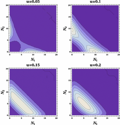
Figure 1. Contour plot of probability distribution P(N1, N2) obtained from stochastic simulations. A Transition from a two peak regime to a one peak regime occurs as the unbinding parameter u increases. g, b and d are kept equal to the E. coli values (4). The line that separates the darkest region in the first picture has a value of 0.005 and every line represents an increase of 0.005, too. In the rest of the pictures, the first line has a value of 0.002 and every line represents an increase of 0.002, as the color gets clearer.
Download figure:
Standard imageTable 1. Value of u for the transition from a bimodal to a unimodal probability distribution. Only one of the parameters g, b, d is changed each time, taking the E. coli values as a reference (4).
| Values of g, b, d | u transition value | Values of g, b, d | u transition value |
|---|---|---|---|
| E. coli | 0.145 ± 0.005 | d = 10−3 | 0.14 ± 0.02 |
| g = 0.015 | 0.345 ± 0.005 | d = 0.01 | 0.295 ± 0.005 |
| g = 0.1 | 0.175 ± 0.005 | b = 0.01 | (4.85 ± 0.05) × 10−2 |
| g = 0.5 | 0.30 ± 0.02 | b = 1.0 | 1.15 ± 0.05 |
| d = 5 × 10⁻⁴ | 0.14 ± 0.02 | b = 3.0 | 3.2 ± 0.2 |
Although the whole probability distribution is always symmetric, distributions P1 and P2 will be a priori asymmetric, since they describe the probability of the number of proteins when a protein 1 or 2 are bound, which are not symmetric situations. Let us now define rA and rB as the probability masses of P1 on either sides of the diagonal N1 = N2:
We can now study how rA, rB change with u, and whether there is a clear transition between the situation in which they are different, and the one in which they are equal to each other (if there is any). Figure 2 shows that these two quantities approach each other in a continuous way, and they are equal only when u → ∞, that is, when the only possible state of the switch is S = 0 and it no longer has any effect on the protein dynamics. Therefore, the probability distributions P1, P2 and hence rA, rB tend to zero, all the probability being concentrated in the distribution P0(N1, N2), which is always symmetric.

Figure 2. Evolution of the two contributions to P1(N1, N2) defined in (5)—rA for N1 > N2 and rB for N1 < N2—as u increases.
Download figure:
Standard imageThe marginal distribution P1 appears to deform continuously into a symmetric distribution when u → ∞. We conclude that (at least for these parameter values) P1(N1, N2) remains asymmetric for u < ∞, and as a consequence so does P2, and there is no transition to a symmetric state in this marginal distribution. As figure 3 shows, P1 has only one peak for different values of u, and even if it becomes smaller as u increases, it does not become symmetric at any point.

Figure 3. Contour plots for the probability distribution P1(N1, N2), for different values of u. As u increases, the peak of the distribution moves towards the diagonal N1 = N2, but the distribution is not completely symmetric as long as u is finite. Also, the probability mass of the distribution decays as u increases, and is transferred to the symmetrical distribution P0(N1, N2). In the pictures, the probability of the points that separates the darkest region, and also the value separation between successive lines is 5 × 10⁻⁵, 10−3, 10−3 and 2.5 × 10⁻⁴, respectively.
Download figure:
Standard imageWe deduce that, even though P(N1, N2) appears to become unimodal at some finite value of u (see figure 1), there is no transition between symmetric and asymmetric regimes, since P1 and P2 always remain asymmetric. Thus, the bistability of the switch is always present, with the asymmetry in distributions P1, P2 decreasing as the switch state becomes less important, that is, as u increases.
2.3. Solution in limit u, b → 0
We now consider the system in the limit u, b → 0 with the binding constant

held fixed. In this limit the system will equilibrate between binding/unbinding events. When the switch is in state 1 the number of type 2 proteins decays to zero and the number of type 1 is given by Poissonian statistics for the generation/degeneration processes:

where r1 is the probability of the switch being in state 1 (r1 = ∑∞N1, N2 = 0P1(N1, N2)). Similarly, in state 2 the number of type 2 is given by Poissonian statistics

and in state 0 both N1 and N2 are given by Poissonian statistics

In order to fix the probabilities r0, r1, r2 we consider the master equation for r1 which can be obtained from summing (2) over the variables N1, N2:

where the quantity 〈N1〉0 is the mean value of N1 given the system is in switch state S = 0, multiplied by the probability of being in switch state S = 0, i.e., 〈N1〉0 = ∑∞N1, N2 = 0N1P1(N1, N2). In the stationary state we have 〈N1〉0 = r0g/d and (10) becomes

A similar equation holds for r2 and the normalisation of probability yields

Thus we see that the system has three long-lived states: when S = 1 the system is dominated by type 1 proteins; when S = 2 the system is dominated by type 2 proteins, and when S = 0 the system is in a symmetric state.
When k → ∞ the symmetric state has zero weight (r0 → 0) and the system is either in the S = 1 state or the S = 2 state. The switching time between the two states is expected to diverge in this limit therefore the system exhibits symmetry breaking. Note that the transition from the S = 1 state to the S = 2 state is through the symmetric S = 0 state.
2.4. Solution in limit u, b → ∞
In this limit the unbinding and binding events happen on a faster time scale than the growth and degradation of proteins. (This may be a physically relevant limit since it is often assumed that binding-unbinding processes are faster than other processes [9].) Therefore, the switch state becomes decoupled from the numbers of protein and the probabilities obey

where P(N1, N2) is the probability of N1, N2 proteins being in the system regardless of switch state, and rS(N1, N2) is the probability for the switch to be in state S, given that the numbers of proteins are N1, N2. That is, for given number of proteins N1 and N2 (which include any bound protein) the switch probabilities equilibrate and obey

which may be solved to obtain

where the binding constant k is given by (6).
A master equation for the evolution of P(N1, N2) on the slower timescale on which generation and degeneration events occur may then be written down:
The terms with coefficient g in (16) represent generation of Ni when the switch is not in switch state i. The terms with coefficient d in (16) represent reduction of Ni with rate dNi when the switch is not state i and reduction with rate d(Ni − 1) when the switch is in state i (this is because the bound protein does not degrade). The stationary state of (16) obeys detailed balance with respect to generation and degradation of N1 and N2 individually, thus
with a similar equation holding for detailed balance in N2. Then these equations may be iterated to obtain
The constant P(0, 0) will be determined by normalisation of the sum of probabilities to one.
The expression (18) is a single-peaked distribution which is symmetric in N1 and N2. To see this one can identify the stationary points of P(N1, N2) through the conditions P(N1 + 1, N2) = P(N1, N2) and P(N1, N2 + 1) = P(N1, N2) which yield
The solution of these equations is N1 = N2 = N/2 which means

and when N is large,

The remaining quadratic

has a single positive root. Thus, in the u, b → ∞ limit the system has reached a symmetric state with the probability distribution peaked at N1 = N2 = N/2 given by (22).
3. Mean field theory
In this section, we develop a mean field theory in which some correlations in the numbers of proteins are ignored.
3.1. Exact moment equations
We start from the exact master equations (1)–(3) for the evolution of probabilities PS(N1, N2). The zeroth moments of Ni are the probabilities rS, i.e.

We now define the first moments of 〈Ni〉S of Ni as follows:

and the second moments

Summing (1) gives


Note that the physical meaning of e.g. 〈Ni〉S is the probability of being in switch state S (rS) multiplied by the mean number of type i, given that the switch is in state S.
Similarly, summing (2) gives


We now invoke symmetry between switch state 1 and 2:

Then the exact steady-state versions of equations (26)–(30) read


Note that if we sum (33)–(35) we obtain the exact relation

which simply gives the overall birth/death balance for N1. Also note that (34) and (35) give exact relations between the second moments and first moments. However, to actually evaluate these moments one would have to consider equations for higher moments, leading to a hierarchy of equations.
3.2. Mean-field approximation
We now make a mean-field approximation that expresses second moments in terms of first moments:


Note that a symmetry condition from (31) has been explicitly used in the last equation of (38). The first relation (37) comes from the assumption that N1 has a Poisson distribution when the switch is in the 0 state. This means that the second moment is equal to the square of the mean plus the mean itself. However, there is an important factor r0, which comes from the fact that 〈N1N1〉0/r0 is the mean square value of N1 given that the switch is in the 0 state and 〈N1〉0/r0 is the mean value of N1 given that the switch is in the 0 state. The Poisson approximation is in fact exact in the limit where u, b tend to zero (see section 2.3).
The second relation (38) is a simple factorization scheme which ignores correlations between the values of N1 and N2 when the switch state is 0.
Using this approximation scheme (34) becomes
and (35) becomes

Using expressions (39) and (40) in (33), combined with the previous approximations (37) and (38) yields the following quadratic equation for 〈N1〉0/r0:

One must take the positive root of this quadratic which yields

Then using (32) one obtains


One may check the limits of section 2 from the quadratic (41). In the limit b, u → 0 with k = b/u one obtains 〈N1〉0/r0 = g/d and ![$r_0 = \big[1 + \frac{2kg}{d}\big]^{-1}$](https://content.cld.iop.org/journals/1751-8121/44/35/355001/revision1/jpa392228ieqn1.gif) in agreement with section 2.3 where it is shown that N1 follows a Poisson distribution with mean g/d when the switch is in state S = 1 or S = 0.
in agreement with section 2.3 where it is shown that N1 follows a Poisson distribution with mean g/d when the switch is in state S = 1 or S = 0.
In the limit b, u → ∞ with k = b/u fixed the quadratic (41) reduces to

This quadratic for  is the same as the quadratic (22) for the value of N = 2N1 that maximises P(N1, N2) in the exact solution of section 2.4.
3.3. Comparison to simulation results
The mean field theory we have developed can be compared with the simulations by studying the zeroth and first order moments of the probability distributions, i.e. r0, 〈N1〉0, 〈N1〉1, 〈N1〉2. (The probabilities r1 and r2 may automatically be obtained from r0, since  .)
.)
Different values of the mentioned quantities are given in table 2, where the parameters of the models have different values. The reference for this table is the set of E. coli values, and only the parameters that are changed are written. For the simulations performed, r0 is always in good agreement with the mean field theory approximation, and so are r1 and r2. Also, 〈N1〉0 is in quite good agreement, too.
Table 2. Results from different quantities from simulations and mean field theory approach. The values of r0 and 〈N1〉0 predicted by the mean field theory are always in good agreement with the simulations. 〈N1〉1 and 〈N1〉2 predictions are quite far from the simulation results, except on the limit u, b → 0, where our approximation is exact.
| E. coli | MFT | u = 0.05 | MFT | |
|---|---|---|---|---|
| r0 | (4.9186 ± 0.0007) × 10−3 | 4.92705 × 10⁻³ |  |
4.54635 × 10⁻² |
| 〈N1〉0 | (2.489 ± 0.005) × 10−2 | 2.48768 × 10⁻² |  |
0.238634 |
| 〈N1〉1 | 4.942 ± 0.008 | 3.74372 |  |
2.71128 |
| 〈N1〉2 | (5.908 ± 0.007) × 10−2 | 1.25604 |  |
2.2774 |
| u = 50, b = 1000 | MFT |  |
MFT | |
| r0 | (4.941 ± 0.004) × 10−3 | 4.95073 × 10⁻³ |  |
2.49872 × 10⁻³ |
| 〈N1〉0 | (2.55 ± 0.06) × 10−2 | 2.48762 × 10⁻² |  |
2.49375 × 10⁻² |
| 〈N1〉1 | 9.89 ± 0.11 | 2.50019 |  |
4.98751 |
| 〈N1〉2 | 0.227 ± 0.013 | 2.49969 |  |
4.97754 × 10⁻⁵ |
〈N1〉1 and 〈N1〉2 are different in the mean field theory, which is an improvement over simpler approximations where they have the same value. However, the values of 〈N1〉1 and 〈N1〉2 are rather different from the simulations, and this comes from ignoring higher correlations of the numbers of proteins and the state of the switch. Only when u, b → 0 are the values in close agreement with the simulation values as expected in this limit where the mean field theory is exact.
Mean field theory can, in principle, be improved by considering higher order moments and correlations. However, the algebra soon gets quite complicated.
4. Exact perturbative solution
In this section, we develop a perturbative approach that allows the steady state probabilities PS(N1, N2) to be computed as a power series in the unbinding rate u.
4.1. Formal solution
We begin by considering the formal solution of the master equation system (1)–(3). To transform the system of equations into a system of partial differential equations, we take the generating function of the different probability distributions:

where S = 0, 1, 2. In this way we obtain a system of linear partial differential equations with non-constant coefficients:


where the right-hand side terms have been set to 0, since the stationary probabilities PS(N1, N2) are the main quantities to be determined in this paper.
The second and the third equations of the system work in a completely analogous way, because of the symmetry of species 1 and 2, so it will be enough to deal with the first two equations. We also note the symmetries K2(z1, z2) = K1(z2, z1) and K0(z1, z2) = K0(z2, z1).
In appendix A we give a formal solution to the system (47)–(49). However, in practice it is not clear how to actually compute e.g. probability distributions from this solution. In order to do this we develop instead a perturbative approach.
4.2. Perturbative approach
In this section we develop a perturbative approach to the problem of finding the exact stationary state. To do so we require a suitable small parameter of the model which we choose to be u, the unbinding parameter. In the u → 0, the exact solution is simple: if, for example, one protein of type 1 is bound, the proteins of this kind will obey the usual Poisson distribution regulated by death and birth terms, while the number of proteins of type 2 will just decay to 0. This limit is the starting point for a perturbative solution, wherein the probability distribution will be expanded in a power series of u:

Owing to the symmetry of the system P2(N1, N2) = P1(N2, N1) we need only consider P0 and P1.
Writing out the expansion explicitly we have
Note that the constant term P(0)0 = 0 since P0 = 0 in the limit of no unbinding.
This approach also makes sense when the typical E. coli values for the parameters are considered [7]:

u is, along with d, the smallest of the parameters. An expansion in 1/b (appendix B) could also be developed, but we find the expansion in u more convenient.
4.3. Zeroth order
In the zeroth order of the u expansion of the stationary master equation (2) (with left-hand side set to zero) we find

We define the generating function

which obeys

the solution of which is independent of z2:

where c1 is a constant to be determined. Analogously  . Applying the normalization condition K(0)1(1) + K(0)2(1) = 1 and the symmetry consideration c1 = c2 leads to

Expanding as a power series in z1, z2 yields

This is a Poisson distribution for N1 with mean g/d, with N2 fixed to be zero. The normalisation factor 1/2 is so that P(0)(N1, N2) = P(0)1(N1, N2) + P(0)2(N1, N2) is normalised to unity.
4.4. General formulation
We substitute the expansion (50) into the stationary master system (1)–(3) with time derivatives set equal to zero. Arranging orders of u the equations may be written as

for S = 0, 1 where the action of the linear operators  is
is
and the inhomogenous terms are


As noted above, we can first determine the zeroth order P(0)1(N1, N2) and P(0)2(N1, N2) = P(0)1(N2, N1) as functions of the parameters of the model. Then, owing to the form of the equation (62), f(1)0 is determined. This allows us to solve for P(1)0 which in turn determines f(1)1 and allows us to solve for P(1)1. Continuing in this fashion the rest of the probabilities will be found following the structure:

In general, P(n)0 will be found before P(n)1.
Having laid out the general perturbation scheme and established the zeroth order (n = 0) solution, we now outline how equations (59) can be solved. We note that for each switch state S the same linear operator  appears at all orders n. This means that the homogeneous parts of the equations are independent of the order (with only the inhomogeneous term on the right-hand side varying between orders) and that they only have to be solved once.
4.5. Green function for 

Let us define a Green function Q0(N1, N2|N01, N02) for the operator  through

so that the solution of (59) may be written

We define a generating function

the equation for which is obtained by summing (65)

with a(zi) = d − (d + b)zi.
In order to solve (68) we use the method of characteristics (see e.g. [28]). The characteristic equations are


where s is a time-like parameter and (69), (70) define characteristic curves along which the partial differential equation (68) reduces to the ordinary differential equation (71). Solving (69), (70) yields the curves

where

and A, B are two constants to be fixed.
Equation (71) can be rewritten as an ordinary differential equation in v as
To integrate (74) we choose an end-point of the integration as v = 1 and set this to correspond to an arbitrary point in the z1–z2 plane. This fixes the two constants A, B as

Thus we obtain
We now expand as a power series in z1, z2 to obtain Q0(N1, N2|N01, N02) from (67)
where I(α, β; x) is defined as the integral

and Γ(z) and 1F1(a, b; z) are the usual Euler Gamma function and confluent hypergeometric function respectively.
4.6. Green function for

If we define a Green function for the operator  through

this equation only has a solution when N2 ≠ 0. To see this we note that summing the left-hand side of (79) over all N1, N2 yields zero, i.e. the operator conserves probability. Therefore, one cannot solve (79) or indeed (59) for an arbitrary right-hand side; one requires that the sum of the right-hand side of (59) over all N1, N2 yields zero. However, since the null space of the operator  is concentrated on N2 = 0 (i.e. the stationary state in (58) is proportional to
  ) we can find a solution of (79) for N2 > 0.
It is simplest to proceed by considering the solution P1 for an arbitrary right-hand side −h(N1, N2)

that satisfies

We define generating functions


then summing (80) yields

In order to solve (84) we again use the method of characteristics. The characteristic equations are this time


Solving the first two equations yields

where now

and A, B are constants to be fixed. The final equation becomes

We choose the integration to be from v = 0 to v = 1 where v = 0 corresponds to z1 = z2 = 1 and v = 1 corresponds to an arbitrary point in the z1–z2 plane which implies A = z1 − 1 and B = z2 − 1. We then obtain the solution of (90)
Expanding as a power series in z1, z2 implies
As discussed above, for N2 > 0 we can define the Green function (79) by means of which the solution of (80) may be written

Then we can read off the Green function from (92) as
For N2 = 0 the solution (92) reads
Some care is required with the r = N1 term of the sum in (95) since the integral I(0, β; x) does not converge. However, the property (81) of the function h implies that the coefficient of the offending integral is zero. To see this one can write the r = N1 term of (95) as
In the final equality, the binomial expansion of (1 − v)p + q has been used with the term s = 0 not present since its coefficient vanishes due to (81). All the integrals in (96) then converge.
4.7. First-order results
The first-order contribution to the stationary probability P(1)0(N1, N2) is given by:

with

Although Q0(N1, N2|N01, N02) is expressed in terms of known integrals in (77), it is advisable to go back to the explicit expression of the integrals (78) to evaluate the sums appearing in (97) more easily. In that way, P(1)0(N1, N2) can be written as:
where the label symm refers to the fact that there will be another term equal to the written one, apart from a switch in the variables N01 and N02.
In appendix C it is shown how the expression may be simplified to the result
Once we have P(1)0, we can plug this result into the P(1)1 equation which becomes for N2 > 0

where f(1)1(N1, N2) = −P(0)1(N1, N2) + b(N1 + 1)P(1)0(N1 + 1, N2).
We consider separately the two terms of f(1)1. The first is

Since the calculation with the Green function (see section 4.6) is only for N2 ≠ 0 this term does not contribute and the only contribution comes from the second term in f(1)1 involving P(1)0. The resulting expression, obtained by substituting h = b(N1 + 1)P(1)0(N1 + 1, N2) in (92) with P(1)0 given by (100), is
where the symmetric term in this case corresponds to the term inside the curly brackets, exchanging the places of N01 + 1 and N02 coming from the symmetric term in P00. For N2 = 0 we obtain the result shown in (95) and cannot be simplified further.
Equations (95), (100) and (103) are the main results of this section and give closed form expressions for the first-order contributions to the stationary probabilities. The normalization constant K(1, 1) appearing in (95) is obtained from the condition:

Once the values of the probabilities P(1)i(N1, N2) have been obtained numerically, they are multiplied by the unbinding parameter u and added to the zeroth order probabilities. In that way, the probability distributions Pi(N1, N2) can be computed and plotted up to the first order of the expansion. Figure 4 shows the probability distributions for different values. The agreement is visually good in the first two examples: typical E. coli values (4) and another interesting case, with smaller g. The order of magnitude is well reproduced in almost every point of the probability distribution. However, the approximation does not work accurately if the value of the unbinding parameter u is of the order or bigger than the other parameters.

Figure 4. Comparison between the analytical first order and the simulation distributions for different values of the parameters (a) E. coli values (4). The probability distributions have the same shape and the order of magnitude is well reproduced in almost every point. (b) g = 0.015, u = 0.0005, d = 0.005, b = 0.1 The order of magnitude is again well reproduced. In this case, the two peaks get closer to the origin as the ratio g/d is smaller. (c) E. coli values with u = 0.05. The approximation at first order is no longer accurate as the value of u is no longer small compared to the rest of the parameters of the model.
Download figure:
Standard imageAlthough the first two examples of figure 4 seem visually in good agreement with the simulations, the best way to check this is to plot different slices of the probability distribution, that is the probability distribution of N2 where N1 is held constant (figure 5). We choose the values of N1 to correspond to the slices with large probability mass, i.e. N1 = 0, 1, 2 for E. coli values. Figure 5 shows that along the slice with greatest probability mass (N1 = 0) the analytical and simulation plots show good agreement. For N1 > 0, there is reasonable agreement for the E. coli values (figure 5(b)), whereas for larger u the agreement is not so good (figure 5(d)).

Figure 5. Comparison between the analytical probability distributions P(N*1, N2) where N*1 is fixed and chosen to correspond to slices with largest probability mass. The agreement in slice N1 = 0 is good for both figures (a) and (c). There is some quantitative difference in (b), which corresponds to the E. coli values in slices with less probability mass. This is improved with second order calculations, as can be seen in figure 6. In (d) the difference is clear, since the first order approximation is no longer accurate, as discussed in figure 4. The error in the values is negligible and, in all the cases, is smaller than the size of the used symbols.
Download figure:
Standard imageSince the proposed method is general, calculations can be performed up to any necessary order to get better results. For example, in the case of E. coli in axes N1 = 1, N2 = 1 is enough to compute the second order to have very good results (figure 6). In general, the method can be iterated as many times as required.

Figure 6. Comparison between the probability slices P(1, N2) and P(2, N2) from second order analytical calculations and simulations, for E. coli values. The second order is clearly enough to get accurate results.
Download figure:
Standard image5. Conclusion
The exclusive genetic switch presented in this paper represents a minimal model of two populations that compete in an indirect way, that is, through a common promoter site that when occupied by a member of one population stops the production of the other. It is a non-equilibrium system because the microscopic processes are irreversible and detailed balance does not hold. The non equilibrium stationary state exhibits interesting properties of bistability, i.e. generically at any given time the system is dominated by one of the populations. We have developed two main analytical approaches to study the stationary state: a mean field theory and an exact perturbative approach. In addition we have presented some exactly solvable limits. We also have studied the system and checked the analytical results by using Monte Carlo simulations.
These simulations show that the system is always bistable, that is, the system is always functioning as a switch, with two opposite states in which one population is much more abundant than the other. This holds generically except in the limit u, b → ∞ where the state is symmetric. As the relevant parameters for the switch become smaller, the probability of finding bound proteins decreases, but the distributions always remain asymmetric, showing no transition between asymmetric and symmetric states.
The mean field theory of section 3 is based on exact moment equations which are factorised at the level of second moments. The approximation scheme is constructed to be exact in the limiting parameter case of vanishing binding/unbinding rates b, u with the binding constant  held constant. The theory shows good agreement with some quantities obtained from the simulation, but there are some other quantities whose agreement varies and depends on the value of the parameters. The mean-field theory could be improved upon by systematically considering higher order moments and correlations.
As a first attempt, to our knowledge, at an exact solution of this nonequilibrium system we have developed an exact perturbative approach which consists of an expansion in the unbinding rate u. We computed the expansion to first order and this has allowed us to obtain the whole probability distribution for the typical E. coli and other values, in good agreement with the simulations. Higher orders can be obtained systematically by iterating the proposed method. The analytical expressions at first order (100), (103) already illustrate the complexity of the nonequilibrium stationary state. In principle, the Green functions that have been calculated in section 4 allow the expansion to be carried out to arbitrary order although analytical expressions for the higher order terms in the expansions might be long or difficult to simplify. However, they still can be computed numerically by programming the proposed operations and, in principle, the method can be iterated as many times as necessary to get more accurate results.
In this paper we have not attempted to study the dynamics, but it would be of interest to do so. In particular the dependence of the flip time or first passage time (the time for the system to change from being dominated by one population to the other) [17] on the parameter values is of interest. It may be possible to extend our analytical solution to consider such flip times and to provide estimate of first passage times between the two bistable states. It might be that the Green functions we have computed in section 4 contain some useful dynamical information.
The techniques that we have developed should be applicable to the understanding of other related systems and properties of genetic switches in general. The factorisation of the moment equation hierarchy is straightforward to implement to obtain a mean field theory; the exact perturbative approach is more involved but can be used in general for problems with similar probability distributions, as long as the Green functions are analytically solvable. Thus the techniques represent standard procedures to analyse this class of systems.
Acknowledgments
Juan Venegas-Ortiz would like to acknowledge the award of a College Studentship from the University of Edinburgh, and would like to thank Francisco Cordobés-Aguilar for useful discussions about numerical implementation of the method.
Appendix A.: Analytical method for systems of linear PDEs
According to [28], there is a way to solve, or at least simplify, a system of linear first-order partial differential equations. First of all, considering a three dimensional space with a vector  for the three probabilities, the system has to be written as

where A, B and C are 3 × 3 matrices, and  and
and  are column matrices. The requirement to solve the system is that detA(z1, z2) ≠ 0 or detB(z1, z2) ≠ 0.
In this case the expression of the matrices is
This is not the most general system that could be written with this notation, since the matrix  is zero, and A and B only depend on z1, z2, respectively.
The requirement to solve the system is that detA(z1, z2) ≠ 0 or detB(z1, z2) ≠ 0, which is fulfilled almost in every point. Multiplying by the matrix B−1, the matrix A is transformed into
whose eigenvalues, written as columns in a matrix R are
This hyperbolic system can be transformed with elementary matrix operations:

The method then states that the components of v obey the following system of equations:
where  are the components of the matrix C' once we have performed the transformation with R:
  .
.
As can be seen from the last equation, we have uncoupled the derivative terms and, even if this system cannot be solved analytically, it is easier to deal with it computationally. The problem itself can be written as
Although this method in principle solves exactly the system of partial differential equations it appears a formidable task to actually integrate equations (A.7).
Appendix B.: Perturbative expansion in 1/b
A perturbative expansion in the parameter 1/b might be performed in the same as the expansion in u. In this case, the explicit expression for the expansion is:
In this case P00(N1, N2) = 0, since in the limit b → ∞, there is no probability to find the system in an unbound state.
In the zeroth order of the 1/b expansion of the stationary master equation (2) (with left-hand side set to zero) we find

which is the same equation as (53). Hence, the zeroth order probability has the solution of equation (58):

As a consequence, the zeroth order of the u and the 1/b expansion are the same. However, higher orders of the expansion in 1/b are much harder to compute than in the u case. For that reason, we have developed the u expansion.
Appendix C.: Derivation of expression (100)
In this appendix we give the detailed derivation of (100). We begin from (99)
where the label symm refers to the fact that there will be another term equal to the written one, apart from a switch in the variables N01 and N02.
Now defining:
we arrive at the expression (for convenience we will drop the dependence of the previous functions on v):
Separating the parts of the expression that can be summed, the following simplification can be obtained by changing the order of the sums appropriately:
where ω = vg/d. Note that this sum could be simplified further, but that the simplification will not allow us to perform the integration over v in closed form. In this and following equation, we will try to obtain the simplest expressions globally, knowing that simplifying one part can lead to further complications in another.
Plugging this sum into the P(1)0 equation and writing all the explicit forms of the functions, we obtain the result (100).