

Abstract
In recent decades, the Barents Sea has warmed more than twice as fast as the rest of the Arctic in winter, but the exact causes behind this amplified warming remain unclear. In this study, we quantify the wintertime Barents Sea warming (BSW, for near-surface air temperature) with an average linear trend of 1.74 °C decade−1 and an interdecadal change around 2003 based on a surface energy budget analysis using the ERA5 reanalysis dataset from 1979–2019. Our analysis suggests that the interdecadal change in the wintertime near-surface air temperature is dominated by enhanced clear-sky downward longwave radiation (CDLW) associated with increased total column water vapor. Furthermore, it is found that a mode of atmospheric variability over the North Atlantic region known as the Barents oscillation (BO) strongly contributed to the BSW with a stepwise jump in 2003. Since 2003, the BO turned into a strengthened and positive phase, characteristic of anomalous high pressure over the North Atlantic and South of the Barents Sea, which promoted two branches of heat and moisture transport from southern Greenland along the Norwegian Sea and from the Eurasian continent to the Barents Sea. This enhanced the water vapor convergence over the Barents Sea, resulting in BSW through enhanced CDLW. Our results highlight the atmospheric circulation related to the BO as an emerging driver of the wintertime BSW through enhanced meridional atmospheric heat and moisture transport over the North Atlantic Ocean.
Export citation and abstract BibTeX RIS

Original content from this work may be used under the terms of the Creative Commons Attribution 4.0 license. Any further distribution of this work must maintain attribution to the author(s) and the title of the work, journal citation and DOI.
1. Introduction
While the Arctic as a whole has warmed more than twice as fast as the rest of the world (Screen and Simmonds 2010a), a phenomenon known as Arctic amplification, the warming has been even more intensified in certain Arctic regions. One such region is the Barents Sea, which has also experienced one of the largest reductions in sea ice extent in recent decades (Chen et al 2016). The meridional heat exchange between the Barents Sea and the North Atlantic Ocean has a strong influence on Barents Sea warming (BSW) and the seasonal sea ice cover over the Barents Sea, which can strongly alter the atmosphere–ocean interactions in this region (Smedsrud et al 2013). The BSW has led to a pronounced upper-ocean warming and a retreating sea ice cover during the 1993–2014 period (Asbjornsen et al 2020) and also caused the reduction of the marine biome and the borealization of fish communities (Fossheim et al 2015, Oziel et al 2020). Moreover, several studies have suggested that the BSW can influence weather and climate extremes in the midlatitudes in winter through changes in the large-scale atmospheric circulation (Cohen et al 2014, Luo et al 2017), and the stratospheric pathway plays a greater role than the tropospheric pathway (Zhang et al 2018). It has been suggested that these circulation changes could act as a positive feedback mechanism that further drives the BSW, which could explain the strong Arctic warming in the early twentieth century (Bengtsson et al 2004). Thus, to improve our understanding of Arctic amplification and its remote effects, it is essential to understand the mechanisms behind the BSW.
Previous studies have attributed the wintertime BSW to different processes, including lapse-rate feedback (Pithan and Mauritsen 2014), cloud feedback due to the increased low cloud cover (Goosse et al 2018) and insulation feedback from sea ice (Boeke and Taylor 2018, Cai et al 2021). Moreover, many previous studies have indicated that the meridional atmospheric and oceanic heat and atmospheric moisture transport from mid-low latitudes have a great influence on the wintertime BSW, which are modulated by the large-scale atmospheric circulation (Chen et al 2013, Woods and Caballero 2016, Hegyi and Taylor 2017, Luo et al 2017, Cho and Kim 2020, Henderson et al 2021, Sang et al 2022). However, most studies explained the BSW from the leading mode of atmospheric variability in the Northern Hemisphere mid- and high-latitudes (Hegyi and Taylor 2017, Cho and Kim 2020, Gao et al 2022) known as the North Atlantic oscillation (NAO) or Arctic oscillation (AO) and there has been little attention paid to secondary atmospheric modes such as the Barents oscillation (BO), which is closely associated with the climate variability in the Barents Sea region (Skeie 2000, Chen et al 2013, Shu et al 2017, Liang et al 2020). Although various processes have been shown to contribute to the BSW, there is still a lack of quantitative studies to determine the dominant factors (You et al 2021), and the exact processes behind the BSW related to the BO changes have so far not been systematically quantified. Therefore, our study aims to quantitatively analyze the variations and causes of the BSW during the 1979–2019 period from the perspective of atmospheric circulations. First, the main factors affecting the BSW were analyzed. Second, the influence and mechanisms of atmospheric circulation on the BSW were investigated. Finally, the changes in atmospheric circulation on the BSW were discussed.
2. Data and methods
In this study, monthly 2 m/skin temperature, sea level/surface pressure, total column water vapor (TCWV), specific humidity, horizontal vector of wind, surface latent/sensible heat flux, surface net downward shortwave/longwave radiation and surface downward shortwave/longwave radiation for all-sky and clear-sky conditions during 1979–2019 were obtained from the ERA5 reanalysis dataset (Hersbach et al 2020), which has a realistic characterization of the spatiotemporal characteristics of Arctic temperature changes (Cai et al 2021). The horizontal resolution of the ERA5 reanalysis data is about 31 km, and the data was obtained on a 0.25° × 0.25° regular grid from the Climate Data Store (https://cds.climate.copernicus.eu).
The horizontal water vapor flux (WVF) represents the amount of water vapor flowing through a unit area per unit time, and the horizontal WVF convergence (WVFC) is the amount of water vapor that converges or divergences per unit time and unit volume. The WVF and WVFC were calculated using the ERA5 data (see supplementary methods 1 and 2 (available online at stacks.iop.org/ERL/17/044068/mmedia) for details). The horizontal temperature advection at 850 hPa was also calculated and decomposed into zonal and meridional temperature advection (supplementary method 3).
Following the method used by Gao et al (2019), we used the moving t-test method to identify the breaking point in the time series of variables, which is based on the mean t-test method to continuously test whether there is a significant difference between two adjacent periods. In this study, the moving step length is 9 years. If the difference between two periods exceeds the significance level of 0.01, it is considered that the mean state has undergone a sudden change, and then the breaking point is obtained (supplementary method 4).
To assess the contributions of different processes to the BSW between two time periods before and after the breaking point over the period 1979–2019, we used the energy budget equation at the Earth's surface proposed by Lu and Cai (2009):
where Q represents the storage of surface heat,  is the surface albedo obtained from the ratio of reflected shortwave radiation (downward shortwave radiation minus net downward shortwave radiation) to incoming shortwave radiation at the surface, SW is the shortwave radiation and LW is the longwave radiation,
  is the longwave emission from the surface (the emissivity,
  , is assumed to be equal to 1, and σ is the Boltzmann constant), and (SH + LH) represent the turbulent heat flux (sum of surface sensible and latent heat fluxes). The perturbation form of equation (1) can be written as,
where Δ represents the change in climatology between the two periods before and after the breaking point (the latter period minus the former period).
The change in the cloud radiative effect (CRE) is calculated as the net radiation difference between all-sky and clear-sky conditions:
where  represents mean state surface albedo for the reference period, and
  ,
,  and
and  indicate cloud-sky, all-sky and clear-sky conditions, respectively.
Combining equations (2) and (3), the final equation can be written as,
In equation (4), the overbar indicates the climatology for the reference period (the former period that was determined by the breaking point) and the surface temperature changes (ΔTs) between the two periods can be decomposed into seven terms, including surface albedo feedback (SAF), change in CRE, the non-SAF-induced change in clear-sky shortwave (SW) radiation, change in clear-sky downward longwave (LW) radiation, change in surface heat storage (Q), changes in turbulent heat flux (SH +LH), and the residual of this decomposition (δ, usually very small) (Lu and Cai 2009). A more detailed derivation of equation (4) is given in the supplementary material. It is worth noting that this method targets the surface temperature and for near-surface air temperature, the contribution of surface heat storage and turbulent heat flux is opposite to that of surface temperature. Nevertheless, the relative magnitude of the terms on the right-hand side of equation (4) can also be interpreted as the relative contribution of each factor to the near-surface air temperature changes.
In addition, monthly wintertime sea-level pressure (SLP) anomalies were decomposed using an area-weighted empirical orthogonal function (EOF) in the region over the North Atlantic and Arctic sector (90° W–90° E and northward of 30° N), and the BO is found to be the second EOF (Skeie 2000, Chen et al 2013). A significance test was performed using the North test (North et al 1982). The main purpose of the limited region is to focus on the internal atmospheric variability of the North Atlantic region, which has a greater impact on the BSW (Chen et al 2013).
3. Results and discussion
3.1. Spatiotemporal characteristics of the BSW and its influencing factors
As shown in figure 1, the wintertime near-surface air temperature in most of the Arctic significantly increased during 1979–2019 with a linear trend of 0.78 °C decade−1. The BSW is accelerated by a linear trend of 1.74 °C decade−1, which is more than twice that of the Arctic. At the same time, the near-surface air temperature changes over the Barents Sea have the largest interannual temperature variability with standard deviations of 3.13 °C. We also verified that changes in near-surface air temperature and surface temperature are very close (figure 1(c)), which justifies the use of the surface energy budget equation for near-surface air temperature changes. The small difference between the two may be due to the near-surface air temperature being affected by horizontal advection in addition to turbulent and radiative fluxes (Kim and Kim 2019, Sang et al 2022).
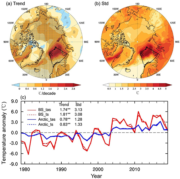
Figure 1. Spatial pattern of (a) near-surface air temperature trend and (b) interannual variability (std) during 1979–2019 in winter (DJF). (c) Time series of Arctic (blue) and Barents Sea (BS, red) averaged wintertime near-surface air temperature (tas, solid line) and surface temperature (ts, dashed line) anomaly (relative to the whole period) during 1979–2019. Hatched regions are statistically significant at the 0.05 level according to the Student's t-test.
Download figure:
Standard image High-resolution imageThe near-surface air temperature, clear-sky downward longwave (CDLW) radiation and TCWV over the Barents Sea had a stepwise jump since 2003 according to the moving t-test analysis (figure 2(a)). To investigate the interdecadal change in the BSW, we analyzed differences between 1979–2002 and 2003–2019 (latter minus former) using the energy budget equation. The regionally averaged mean surface temperature (near-surface air temperature) increase during the latter period is 4.4 °C (4.4 °C) relative to the former period. As shown in figure 2(b), the BSW is dominated by the enhanced CDLW (contributions of 3.6 °C to the surface temperature change), which represents the net effect of changes in the atmospheric water vapor, CO2 concentration and air temperature (Lu and Cai 2009, Gao et al 2019). Among these factors, the effect of atmospheric water vapor changes plays a major role, which is reported to be more pronounced over high latitudes than in other regions (Clark et al 2021). Therefore, the contribution of CDLW to the BSW is considered to come from atmospheric water vapor changes affected by local evaporation and poleward transports (Zhang et al 2013, Cho and Kim 2020), which can also be derived from the simultaneous changes of near-surface air temperature, CDLW and TCWV, as shown in figure 2(a). Surface heat storage exhibits the second strongest BSW contributions (1.5 °C). Changes in the turbulent heat flux are the third-largest contributor (−1.1 °C) and had a cooling effect on the surface, which is related to the increase in the open sea and the enhancement of atmosphere–ocean interaction due to the retreat of sea ice (Screen and Simmonds 2010b, Shu et al 2021). The change in the CRE contributes to a minor part of the temperature change and is only 0.4 °C. Furthermore, SAF, as well as shortwave radiation effects, are negligible in winter due to the absence of solar radiation.
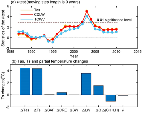
Figure 2. (a) Moving t-test of the wintertime (DJF) near-surface air temperature (yellow), CDLW radiation (red) and TCWV (blue) in the selected region. Black dashed line represents the 0.01 significance level. Period 1979–2019 is divided into two periods according to the moving t-test method (1979–2002 and 2003–2019). (b) Near-surface air temperature (Tas), surface temperature (Ts) and the partial temperature changes due to the changes in SAF, CRE, SW (clear-sky downward shortwave radiation). LW (clear-sky downward longwave radiation), Q (surface heat storage), and SH + LH (the sum of turbulent sensible and latent heat fluxes) between the 1979–2002 and 2003–2019 period in winter.
Download figure:
Standard image High-resolution image3.2. Link between the BSW and atmospheric circulations
The first two leading EOFs of monthly wintertime SLP anomalies during 1979–2019 from the ERA5 reanalysis data set are shown in figure 3. EOF1 is the NAO with the Azores high- and Icelandic low-pressure centers (figure 3(a)), which accounts for 47.0% of the total variance in the selected region and can be well separated from the other modes (North et al 1982). EOF2 is called the BO, which has two primary centers of action over the South of the Barents Sea and the North Atlantic Ocean, and a slightly opposite sign center around Greenland (figure 3(b)). This mode accounts for 16.8% of the total variance and is also a robust mode of climate variability (Chen et al 2013).
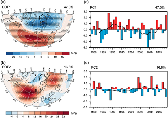
Figure 3. First two EOFs of winter (DJF) SLP anomalies (hPa) in the selected region from 1979–2019 and their corresponding principal components (PCs). All patterns pass the North test. (a), (b) Linear regression of winter SLP on PC1 and PC2. Hatched regions are statistically significant at the 0.05 level according to the Student's t-test. (c), (d) The time series of standardized PC1 and PC2. The black lines represent the 9 year moving average.
Download figure:
Standard image High-resolution imageThe near-surface air temperature anomalies linked to the interannual variability of the two PCs are shown in figure 4. The positive NAO phase corresponds to widespread warming over Eurasia and eastern North America, and cooling over the Greenland–Baffin Bay Seas (figure 4(a)). The positive BO pattern is associated with BSW, along with two cooling centers over Europe and northern East Asia (figure 4(b)). PC2 is also known as the BO index and shows the strongest temporal correlation with near-surface air temperature over the Barents Sea (r = 0.51, p < 0.05), indicating a close linkage between the BO and the wintertime BSW, whereas, the relationship between the BSW and the NAO is weak and insignificant (PC1: r = 0.01, p > 0.05) (figure 4(c)).

Figure 4. Linear regression of winter (DJF) near-surface air temperature (°C) on SLP (a) PC1 and (b) PC2. Dotted regions are statistically significant at the 0.05 level according to the Student's t-test. (c) Time series of standardized PC1 and PC2, and average near-surface air temperature over the Barents Sea.
Download figure:
Standard image High-resolution imageFigure 5 displays the composite differences in winter mean fields between the high and low years of the two SLP-PCs. During the positive BO phase, high-pressure anomalies are found near the North Atlantic Ocean and the Barents Sea. The anticyclones facilitated two branches of water vapor transport from southern Greenland along the Norwegian Sea and from the Eurasian continent to the Barents Sea, which converged over the Barents Sea (figure 5(f)). The increase in water vapor content over the Barents Sea caused the BSW through increased CDLW (figures 5(b) and (d)). Meanwhile, the atmospheric meridional heat transport also increased, which can be derived from the significant positive temperature advection anomaly over the Barents Sea (figure 5(h)). The downward anomaly of the turbulent heat flux (not shown) during the positive BO phase suggests that the atmosphere drives the sea ice loss at this time (Blackport et al 2019). Since the NAO is predominantly associated with zonal winds, it is not significantly correlated with the poleward heat and moisture transport to the Barents Sea, and hence no significant warming is found over the Barents Sea (figures 5(a), (c), (e) and (g)).
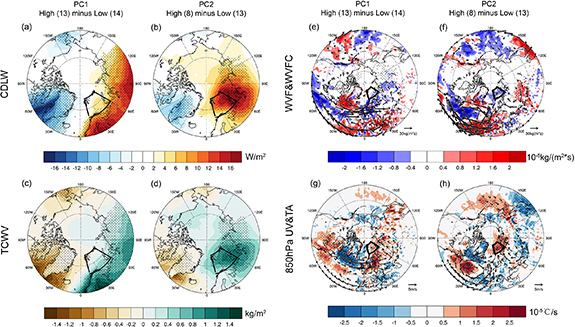
Figure 5. Composite differences in (a), (b) CDLW radiation (units: w m−2), (c), (d) TCWV (units: kg m−2), (e), (f) WVF (units: kg (m·s)−1) in the whole layer and their divergences (WVFC, shading; units: 10−5kg (m2·s)−1) and (g), (h) 850 hPa wind (UV, units: m s−1) and temperature advection (TA, units: 10−5 °C s−1) in winter (DJF) between the high (above +0.5 standard deviation) and low (below −0.5 standard deviation) PC1/PC2 years (former minus latter) from figure 3. Numbers in parentheses indicate the number of years with high and low PCs. Dotted regions are statistically significant at the 0.05 level according to the Student's t-test.
Download figure:
Standard image High-resolution image3.3. Interdecadal changes in the BO have led to a stronger BSW since 2003
As shown in figure 6(a), the BO index had undergone a significant interdecadal change around the winter of 2002/2003, from the negative phase to the positive phase, which was consistent with the observed jump in temperature over the Barents Sea. During the former period (1979–2002), the atmospheric circulation was dominated by the NAO (figure 6(b)). Although the explained variance by NAO reached 48.7%, it made little contribution to the BSW (r = 0.18, p > 0.05) (figure 6(c)). Meanwhile, the BO mode did not appear in the second EOF. During the latter period (2003–2019), the BO with its meridional structure became evident and shifted to a positive phase with the explained variance of 21.4% (figure 6(b)), and the linkage with the BSW was also strengthened (r = 0.54, p < 0.05) (figure 6(c)). The enhanced meridional atmospheric circulation during the latter period contributed to the stronger BSW relative to the former period, indicating an interdecadal strengthening of the BSW modulated by the interdecadal variation of the BO.

Figure 6. (a) Moving t-test of the near-surface air temperature (yellow), PC1 index (blue) and PC2 index (red) of wintertime (DJF) SLP. Purple dashed line represents the 0.01 significance level and the black dashed line represents the 0.05 significance level. (b) First two EOFs of winter SLP anomalies (hPa) in the selected region during the 1979–2002 and 2003–2019 periods. (c) Scatter diagram of wintertime near-surface air temperature (Tas) over the Barents Sea against PC1/PC2 index.
Download figure:
Standard image High-resolution imageThe differences in the mean state of the atmospheric circulations between the two periods are mainly manifested in the increase in SLP in northern Eurasia and the strengthening of the 500 hPa geopotential height near the Barents Sea during the latter period (not shown). This is reminiscent of the recovery of the intensity of the Siberian High (from the former weakening to the latter strengthening) (Jeong et al 2011) and the increased frequency and persistence of Ural blocking since the mid-2000s (Luo et al 2016, Chen et al 2018). These changes may have contributed to the strengthening of the anticyclone on the east side of the BO during the latter period, and the BO shifting to the positive phase strengthened the poleward heat and moisture transport to the Barents Sea (figure 7). In fact, the effect of the positive phase of the BO in our study is similar to the conclusion of Luo et al (2017), who proposed that the combination of wintertime Ural blocking and the positive phase of the NAO led to the strongest BSW and sea ice decline (Luo et al 2016, 2017). Other studies have also pointed out that the influence of poleward heat and moisture transport changes associated with such changes in atmospheric circulation on the wintertime BSW has become more important in recent years (Woods et al 2013, Gong and Luo 2017, Wang et al 2020, Henderson et al 2021).

Figure 7. Schematic diagram of the influence of a positive phase BO on the winter BSW. Anticyclone in the dotted line became significant during the latter period, which facilitated the poleward heat and moisture transport along the Norwegian Sea. Increase in convergence of water vapor amplified the BSW through CDLW.
Download figure:
Standard image High-resolution image
4. Summary and concluding remarks
In this study, we quantified the causes of the wintertime BSW during 1979–2019 through a surface energy budget analysis and further explored the atmospheric circulation associated with the BSW. The main findings are summarized as follows:
- (a)The wintertime BSW is amplified with an average linear trend of 1.74 °C decade−1 during 1979–2019. There was a significant stepwise jump in the BSW in 2003. Enhanced CDLW is the leading factor of the BSW between the two periods before and after the stepwise jump (1979–2002 and 2003–2019), which is dominated by the changes in water vapor over the Barents Sea. The influence of surface heat storage and upward turbulent heat flux are the second-largest contributors to the BSW, while the influences of CRE and SAF are minimal.
- (b)BO is the most important atmospheric mode affecting the near-surface air temperature over the Barents Sea, which is strongly related to the meridional flow over the Norwegian Sea. The positive BO phase is associated with the enhancement of poleward atmospheric heat and moisture transport and enhanced water vapor convergence over the Barents Sea, which amplifies the BSW through CDLW.
- (c)The BO has trended towards a positive phase since 2003, that is, the anticyclones near the Barents Sea and the North Atlantic have strengthened, which would be more conducive to transporting atmospheric heat and moisture to the Barents Sea. Meanwhile, the transition time of the BO index is consistent with the observed jump in near-surface air temperature over the Barents Sea, and the correlation between them has also increased since 2003, suggesting that the wintertime BSW is greatly affected by the atmospheric circulation-related changes in the BO.
This study emphasizes the BO as an emerging driver of wintertime BSW during 1979–2019, contributing to the stepwise jump since 2003. However, whether the BSW and the BO are jointly driven by global warming, and the causal relationship, as well as the interaction between them, need to be further studied. In addition, the wintertime BSW is not constrained to the atmosphere but extends throughout the water column, especially over the northern Barents Sea (Lind et al 2018, Shu et al 2021), which is closely related to the role of oceanic changes (Polyakov et al 2017). During our study period, the ocean heat transport through the Barents Sea Opening (71° N–76° N, 20° E) increased, along with increases in ocean heat content and sea surface temperature in the Barents Sea, which accelerated sea ice area reduction. The increased turbulent heat flux from the ocean to the atmosphere could have promoted the BSW. This phenomenon, known as Atlantification, is a non-negligible factor in the sea ice reduction and warming in the Barents Sea (Polyakov et al 2017, Arthun et al 2019, Asbjornsen et al 2020). However, ocean heat transport cannot explain the stepwise jump since 2003 (figure S1). Therefore, it is the interdecadal changes in the BO that have led to a stronger BSW since 2003. Nonetheless, we still need to note that BSW is caused by the combined effect of atmospheric and oceanic processes, and it is worth investigating their relative contributions in future studies.
Acknowledgments
This work is supported by the National Natural Science Foundation of China (Grant Nos. 41790472 and 41971072). Support from the Swedish Foundation for International Cooperation in Research and Higher Education (CH2019-8377 and CH2020-8799) is also acknowledged. J Cohen is supported by the US National Science Foundation grants PLR-1901352 and ARCSS-2115068.
Data availability statement
The data that support the findings of this study are openly available at the following URL/DOI: https://climate.copernicus.eu/climate-reanalysis.