

Abstract
India's land transport GHG emissions are small in international comparison, but growing exponentially. Understanding of geographically-specific determinants of GHG emissions is crucial to devise low-carbon sustainable development strategies. However, previous studies on transport patterns have been limited to socio-economic context in linear and stationary settings, and with limited spatial scope. Here, we use a machine learning tool to develop a nested typology that categorizes all 640 Indian districts according to the econometrically identified drivers of their commuting emissions. Results reveal that per capita commuting emissions significantly vary over space, after controlling for socioeconomic characteristics, and are strongly influenced by built environment (e.g. urbanization, and road density), and mobility-related variables (e.g. travel distance and travel modes). The commuting emissions of districts are characterized by unique, place-specific combinations of drivers. We find that income and urbanization are dominant classifiers of commuting emissions, while we explain more fine-grained patterns with mode choice and travel distance. Surprisingly the most urbanized areas with highest population density are also associated with the highest transport GHG emissions, a result that is explained by high car ownership. This result contrasts with insights from OECD countries, where commuting emissions are associated with low-density urban sprawl. Our findings demonstrate that low-carbon commuting in India is best advanced with spatially differentiated strategies.
Export citation and abstract BibTeX RIS

Original content from this work may be used under the terms of the Creative Commons Attribution 3.0 licence. Any further distribution of this work must maintain attribution to the author(s) and the title of the work, journal citation and DOI.
1. Introduction
The IPCC indicates that rapid reduction of greenhouse gas (GHG) emissions is necessary to keep temperatures below 2 °C (Edenhofer et al 2014). In 2010, over one-fifth (∼23%, 6.7 GtCO2) of total energy-related emissions originated in the transportation sector (Kahn Ribeiro et al 2012, Sims et al 2014). Moreover, transportation sector's contributions to overall GHG emissions are growing, both in absolute and relative terms, as structural change shifts activity from industry to service sectors (Schäfer 2005). Rapid decarbonization is also challenged by the (perceived) high costs of decarbonizing transport, requiring high energy-density fuels (Creutzig 2016). Nonetheless, halving CO2 emission from transport by 2050 from 2010 levels could be feasible, if not only electric two-, three- and four-wheeler rapidly penetrate into motorized transport markets, but if urbanization dynamics also shift towards more compact urban form (Creutzig et al 2015).
Emerging and rapidly urbanizing countries, like India, provide major opportunities to shape transport systems and infrastructure around low-carbon options (Shukla et al 2008, Bongardt et al 2013; Doll et al 2013). These options have significant co-benefits, such as reducing air pollutants (Xia et al 2015), enhancing population health through physical activity (Woodcock et al 2009, de Sá et al 2017), energy security (Dhar and Shukla 2015), and possibly alleviating poverty (Starkey 2002). In particular, air pollution is a major motivation, as 660 million Indians are estimated to live in areas with health-unsecure levels air fine particulate matter, reducing life expectance in averagy by more than 3 years (Greenstone et al 2015). Often these co-benefits outweigh the benefits of decarbonization in transportation's sector (Creutzig and He 2009, Schipper et al 2011, World Health Organization 2011, Creutzig et al 2012).
India's motorized vehicle growth has increased exponentially over time, and is dominated by two-wheeler (figure 1(a)) that led to exponential increase in the road transport sector's GHG emissions (figure 1(b)). Dhar et al (2018) estimated that Indian transport sector energy demand would increase by 4.5 times, 2.7 times, 2.4 times, and 1.7 times in Business As Usual, Nationally Determined Contributions, 2 °C, and 1.5 °C scenarios respectively by 2050 compared to 2015 levels. Notably, Dhar et al suggest that deep decorbonization in the transport sector, such as envisaged in 2 °C or1.5 °C scenarios, will require both demand and supply side policy interventions, including transformative human behaviors relying on information technology, internet and the sharing economy, the electrification of the transport sector, and innovations in national and sectoral policies, including decarbonization of electricities and explicit carbon prices.
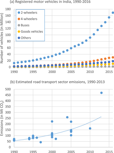
Figure 1. (a) Growth trend in registered motor vehicles, 1990–2016. (b) Estimated road transport sector emissions in India, 1990–2013. Four-wheeler includes cars, jeeps and taxis. Trend analyses show exponential growth in vehicles and related emissions over time. Source: (a) Ministry of Road Transport & Highways MORTH (2018); (b) from various studies, as cited in Singh et al (2019).
Download figure:
Standard image High-resolution imageGiven the high and growing share of carbon emissions from the transport sector, several studies have been conducted to deepen the understanding on transport-based GHG emissions, particularly, its measurements and compositions, geographic/spatial variations, and determinants or correlates. Major transport-based studies on GHG emissions used aggregate level assessment, as those from the International Energy Agency's studies (IEA 2009), and integrated assessment modelling (Edelenbosch et al 2017, Dhar et al 2018). Studies using bottom-up approach utilized disaggregated GHG emissions, such as activity-based (e.g. work, leisure) (Millard‐Ball and Schipper 2011, Jones and Kammen 2014), or mobile sources based (e.g. road, aviation, railways, and navigation) (MoEF 2010). Geographic/spatial variations of transport-based GHG emissions are mostly focused on region and country (Streets et al 2003, IEA 2009, MoEF 2010). A few studies, but growing in number, investigated transport-based GHG emissions at subnational level, including the state level (Ramachandra and Shwetmala 2009), the city level (Ahmad et al 2015) and the sub-city level (Wang et al 2017). Studies have also identified and quantified determinants of GHG emissions at individual or household level (Ahmad et al 2015, 2017), and often spatially aggregated level (Marcotullio et al 2012, Guo et al 2014). Other studies measured vehicle miles travelled (Cervero and Murakami 2010), person miles travelled (Krizek 2003, Jain et al 2018, Korzhenevych and Jain 2018), or transport expenditure (Ahmad et al 2016), proxies of transport-based GHG emissions. While these studies provide valuable insights about correlates of transport-based GHG emissions, one of the characteristics features of these studies is the use of aspatial (stationary) analysis methods such as multivariate regression that do not allow for variations of coefficients over space.
Given significant socio-spatial variation across Indian districts, we hypothesize that major determinants of transportation emissions vary widely over space. This study aims (a) to understand spatial pattern/typology of commuting GHG emissions in India, and (b) to identify its correlates in spatial context (district level). To address these issues, we investigate spatially explicit data of commuting patterns employing tree regression to identify typology of commuting GHG emissions.
2. Methods
We describe first the regression model linking commuting emissions with it determinants, and then the recursive partitions method used to identify the different types of districts (each of which is subject to a separate regression). Throughout the process, we also test and validate models, wherever needed.
We start our analysis of the determinants of commuting emissions with the standard regression equation:

where,  is commuting emissions for district j,
  are determinants factors, and
  is the classical error term representing the effects of unobserved variables. Determinants factors consist of built environment (urbanization level, travel time to nearest city, population density, and road density), mobility related variables (travel distance, travel modes, and fuel prices), and socio-economic characteristics (GDP, and literacy rate). Four variables—commuting emissions, population density, road density, GDP—are considered in their logarithmic transform respecting the distribution of data, and following the econometric literature on this topic (Ahmad et al 2015, Baiocchi et al 2015).
For developing typology of districts with respect to drivers of commuting emissions, we use the classification and regression tree (CART) methods developed by Breiman et al (1984), that iteratively partitions the data into homogeneous subgroups, by fitting separate regression model at each node (equation (1)). We use a regression tree approach since we want to predict the values of a continuous variable, commuting emissions, in different spatial and socio-economic contexts. The algorithm of CART is structured as a sequence of questions, which resulted into a tree like structure, where the ends are terminal nodes that correspond to types of commuting patterns according to spatial context. CART has three main elements: rules for splitting data at a node based on the values of one variable; stopping rules of splitting; and prediction for the target variable in each terminal node. At each split, the available sample is partitioned into two groups by maximizing an information measure of node homogeneity and selecting the covariate showing the best split. The split can be presented, as a binary decision tree where the branch on the right of each non-terminal node contains the districts for which split variable is greater than the split value. CART provides computationally efficient strategies for estimating non-parametric regression model (for detail discussion see Baiocchi et al (2015)).
To avoid overfitting, a large tree is grown first and then reduced in size by a pruning process. Given the flexible non-parametric approach, it is possible to fit a tree with many parameters, including noisy features, which may render to some degree arbitrary and unsuitable for generalization and interpretation. Here, we hence improve the predictive ability of a tree of a specific size by using a technique known as cross-validation. Tree size is optimized by minimizing the cross-validated error.
Alternatively, we have also used geographically weighted regression to assess determinants of commuting emissions spatially to validate our overall findings from the tree regressions (see SI is available online at stacks.iop.org/ERL/14/045007/mmedia). In general findings from both methods agree on the key findings. However, we chose tree regression as the main method for this paper as tree regression allows for relatively straight-forward interpretation and enables the construction of policy-relevant typologies. These analyses were performed using R, a free programming language and software environment for statistical computing and graphics.
2.1. Data
The commuting data were taken from the Census of India enumeration on 'other workers by distance from residence to place of work and mode of travel to place of work' (Census of India 2011a). Here 'other workers' are those persons whose main activity was ascertained according as their time spent as a worker producing goods and services or as a non-worker other than those (a) working as cultivator, (b) working as agricultural labourer, and (c) working at household industry. This commuting data is disaggregated by location (urban and rural), gender (male and female), and distance ranges at district level. Travel mode shares related data include walk, bicycle, two-wheeler, four-wheeler, three-wheeler, bus, train, and water transport or their groups, which are active transport (walk and cycle), motorized transport-private (two-wheeler and four-wheeler), and motorized transport-public (three-wheeler, bus, train, and water transport). We have used this data for calculating annual per capita commuting emissions (kg CO2/p/yr) as follows:
where i represents mean daily distance ranges in kilometer (e.g. 0.5 km for 0–1 km range; 3.5 km for 2–5 km range; 8 km for 6–10 km range; 15.5 km for 11–20 km range; 25.5 km for 21–30 km range; 40.5 km for 31–50 km range; and 60.5 km for 51 + km range), and j represents transportation modes (e.g. two-wheeler, bus). To represent the return trip, emissions were multiplied by 2. Values were converted to annual emissions by assuming 300 mean working days. Further divided by district population to calculate per person emissions. Emission factor for travel mode were taken from data of the India GHG Program (2014) in kg CO2/km (or kg CO2/passenger-km for pblic transport modes such as bus) (see table S1).
Major explanatory variables data were extracted from publicly available sources (table 1). Road density, for instance, is calculated from the road network data from the Open Street Map, a collaborative project to generate a free map of the world based on crowed-source data (openstreetmap.org).
Table 1. Descriptive summary of the study population India, 2011.
| Variable | Mean | St. Dev. | Min | Max | Data source |
|---|---|---|---|---|---|
| Dependent variable: | |||||
| Commuting emissions, kg CO2/person/year | 20.0 | 18.9 | 1.8 | 140.4 | Authors' calculation based on Census of India (2011a) |
| Independent variables: | |||||
| Built environment | |||||
| Urbanization level, % | 26.4 | 21.1 | 0.0 | 100.0 | Census of India (2011b) |
| Travel time nearest city, min | 68.7 | 137.9 | 0.0 | 1,169.3 | Authors' calculation from Weiss et al (2018) |
| Population density, persons/km2 | 934.4 | 3,025.3 | 1 | 37,346 | Census of India (2011b) |
| Road density, km/km2 | 0.7 | 1.9 | 0.02 | 22.8 | Authors' calculation from the Open Street Map (June) 2017 |
| Socio economic characteristics | |||||
| GDP, ₹/cap | 38 830 | 30 197 | 5,198 | 411 633 | State's planning department (c.2011) |
| Literacy rate, % | 72.3 | 10.5 | 36.1 | 97.9 | Census of India (2011b) |
| Mobility-related variables | |||||
| Commuting distance, km | 5.9 | 1.9 | 1.3 | 14.0 | Census of India (2011a) |
| Walk share, % | 13.2 | 8.3 | 3.1 | 57.3 | -do- |
| Bicycle share, % | 14.4 | 10.0 | 0.4 | 45.8 | -do- |
| Active transport, % | 27.6 | 11.8 | 5.6 | 68.3 | -do- |
| Three-wheeler share, % | 4.6 | 3.5 | 0.4 | 24.5 | -do- |
| Bus share, % | 31.6 | 16.7 | 0.6 | 74.2 | -do- |
| Train share, % | 11.2 | 11.2 | 0.01 | 70.1 | -do- |
| Water transp. share, % | 0.7 | 2.4 | 0.0 | 36.9 | -do- |
| Motorized transport-public, % | 48.1 | 15.5 | 7.3 | 85.5 | -do- |
| Two-wheeler share, % | 15.9 | 7.9 | 0.7 | 41.6 | -do- |
| Four-wheeler share, % | 6.3 | 6.3 | 0.5 | 46.5 | -do- |
| Motorized transport-private, % | 22.2 | 9.2 | 3.5 | 49.5 | -do- |
| Diesel price, ₹/l | 46.2 | 1.7 | 42.2 | 48.6 | Ministry of Petroleum & Natural Gas, as cited in Lok Sabha Secretariate (2013) |
| Valid N | 640 | ||||
Note: 1 US$ = 44.7 US$ on 31 March 2011.
3. Results
India's mean annual commuting emissions (home to/from work) is 20 kg CO2 per capita, with the highest (140 kg CO2) in Gurgaon district (Haryana) and the lowest (1.8 kg CO2) in Shrawasti district (Uttar Pradesh) (table 1 and figure S1). The mean urbanization level is 26.4%, but varies immensely from null (e.g. Kinnaur district, Himachal Pradesh) to 100% urban population (e.g. Mumbai district, Maharashtra). The average travel time to the nearest urban center is about 69 min, but it can be as high as 20 h for inhabitants in remote disctricts. The mean district density is 934 p km−2 (SD =3025 p km−2), with the highest 37 000 p km−2 in North East district (Delhi), and the lowest one p km−2 in Dibang Valley district (Arunachal Pradesh). The road density varies between 0.02 and 22.8 km km−2, with mean 0.7 km km−2. The mean district GDP per capita is 39 000 ₹ (circa 2011), with a minimum of 5200 ₹ in Sheohar district (Bihar) and a maximum of 411 000 ₹ in Mumbai district (Maharashtra). The mean commuting distance (among commuters) is 5.9 km, with the lowest 1.3 km in Longleng district (Nagaland) and the highest 14 km in Dharmapuri district (Tamil Nadu). Roughly, annual per capita commuting mobility (mean travel distance/day = 9.007 km) is about 58% of per capita passenger mobility 5685 km (Dhar and Shukla 2015). There is a huge variation in travel mode choices in Indian districts, for instance, four-wheeler share between 0.5% and 47% and active transport (walking and cycling) share between 6% and 68%. In the following, we present seven insights of our analyses.
First, income and urbanization are the key drivers of the district typology with respect to commuting emissions (figure 2). Income is the best discriminator for a typology of districts with respect to commuting emissions. The split based on income occurs at the threshold of about 28 000 ₹/capita. In the high-income part of the tree (nodes 12, 13, 14, and 15) urbanization is the dominant discriminatory attribute splitting clusters at about 43% level. However, urbanization is not a discriminator in low-income district types.
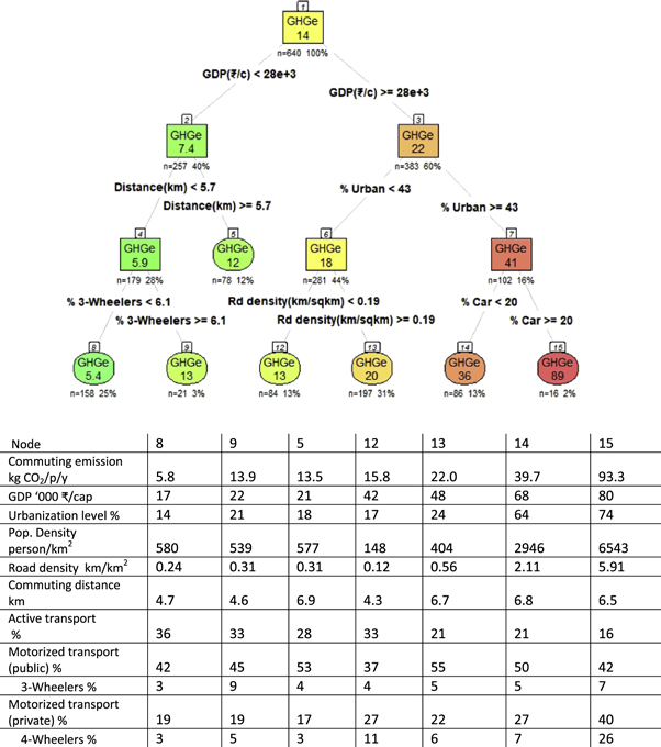
Figure 2. District types in India as determined by their Commuting CO2 emissions drivers. Key statistics are given for each type in the table below (% values are rounded to the nearest whole number, GDP values rounded to the nearest thosand). CO2 emissions drivers split districts recursively to produce maximally distinct district types. Rectangles indicate the splitting criteria in terms of splitting variable and threshold value of splitting variable; Ovals are terminal nodes which represent the different district types and contain the estimated subsamples (see figure 3). Values inside the rectangles or ovals represents average commuting emissions for respective type/node in kg CO2. Small square above rectangles or ovals represent node number, figure 3 maps final nodes that are in oval shape. N represents number of districts at that node and parallel figure in % represents percentage of total districts.
Download figure:
Standard image High-resolution imageSecond, average commuting emissions are highest for districts with high-income inhabitants, that are highly-urbanized, and that heavily rely on four-wheeler for commuting (node 15), and lowest for districts with low-income, have shorter commuting distance, and rely least on three-wheeler for commuting (node 8). These patterns contrast with observations from countries like the United States, where commuting emissions are highest in low-dense settlements (suburban or rural) (Grubler et al 2012, Jones and Kammen 2014). Within high-income and highly-urbanized districts, reduced reliance on four-wheeler for commuting (<20%) cuts average commuting emissions by 60% from 89 kg CO2 (node 15) to 36 kg CO2 (node 14). Similarly, within low-income districts, shorter commuting distance (<5.7 km) cuts average commuting emissions by 51%, 12 kg CO2 (node 5) to 5.9 kg CO2 (node 4), and within low-income, and shorter commuting district, reduced reliance on three-wheeler (<6.1%) cuts average commuting emissions by 58%, 13 kg CO2 (node 9) to 5.4 kg CO2 (node 8).
Third, commuting emissions drivers' impact is not homogeneous, but context dependent (figure 2 and table S3). Thus emission drivers for commuting cannot be adequately explained by a unique global model (table S2), as also argued by Baiocchi et al (2015) for residential CO2 emissions in England. The impact of urbanization level on commuting emissions shows strong variability over the study area in expected positive directionality. A one percentage point increase in urbanization is associated with increase in commuting emissions between 0.5% (node 14) and 2% (node 5). Similarly, income has spatially varying influence in increasing commuting emissions: a 1% increase in income is associated with increase in commuting emissions between 0.35% (node 8) and 0.40% (node 5). Commuting emissions also increase with road density; a 1% increase in road density is associated with increase in commuting emissions between 0.07% (node 14) and 0.24% (node 8). The impact of commuting distance on commuting emissions shows again strong variability in expected positive directionality. A 1 km increase in commuting distance could increase commuting emissions between 4.3% (node 13) and 20.5% (node 12). These heterogeneous relationships indicate that most of the explanatory variables have higher magnitude of influence in currently low emitting districts/regions (nodes 8, 9 and 5), for instance, urbanization, population density, road density, and GDP.

Figure 3. Human settlement type, as characterized by its commuting emission drivers in India. Each district is colored according the corresponding node from the tree regression results it belongs to earlier figure 2.
Download figure:
Standard image High-resolution imageAs expected fuel price is negatively associated with commuting emissions, but only in low-income districts (table S2) or specifically in Node 9 and 12 (table S3). With a 1 ₹ increase in diesel price, commuting emissions decrease by 11% in node 9, and 10% in node 8 (table S3), whereas aggregate 3% in low-income districts (table S2). Given these districts have least commuting emissions and low socio-economic status (figure 2), our study finds limited support for increasing gasoline prices as a strategy to mitigate commuting emissions. Rather increasing gasoline price would burden mobility among low socioeconomic status' population. However, increasing transport fuel prices in Indian metropolitan areas has been identified as a strategy to improve public health (Ahmad et al 2017).
Fourth, per capita commuting emissions decrease with increase in population density, except in node 5 where commuting emissions increase with increase in population density, but with lesser statistical significance (p < 0.1) (table S3). On average, a 10% increase in densification reduces commuting emissions by 1.1%, ceteris paribus. Figure 4 reveals residents living in dense areas (mostly among metropolitan regions) are affluent and that contribute to higher per capita commuting emissions. However, there are several regions (e.g. Gurgaon and Faridabad) that have high per capita commuting emissions but relatively low population density. Mostly, these regions fall in nodes 14 and 15 that have high motorized transport share as well as high road density, hence road congestion (figure 2). This suggests increasing population density with appropriate transportation systems (e.g. active transport and public transport) could reduce commuting emissions in a few regions, mostly across metropolitan regions.
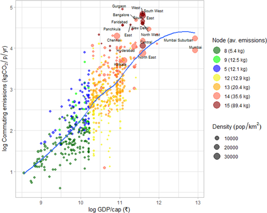
Figure 4. Comuting emissions per capita increases with increasing economic activity. Residents living in higher density regions are very affuluent, and have higher per capita commuting emissions (e.g. metropolitan regions). However, there are several regions with low density but higher per capita commuting emissions (e.g. Faridabad, Gurgaon, North Goa, and South Goa). Scatterplot smoothing uses local regression method 'loess'. The National Capital Territory of Delhi has following districts (mostly labelled): Central, North, South, East, North East, South West, New Delhi, North West and West.
Download figure:
Standard image High-resolution imageFifth, the mean per capita commuting emissions of the district typologies vary by a factor of 16.5. Variance in per capita commuting emissions is higher for high-income districts (factor of 6) than for low-income districts (factor of 2.5). This could be partially explained by the variation in income, urbanization level and transport mode choices between high- and low-income district typologies (see figures 2, 4, and 5). Importantly, districts with similar emissions may have emissions driven by a different set of determinants. For example, nodes 5, 9 and 12 have similar average emissions (12, 13, and 13 kg CO2/cap respectively). However, node 5 is characterized by low income, and long distances, node 9 by low income, short distances, and a high number of three-wheeler, and node 12 by high income, low urbanization, and low road density (figure 2). This result emphasizes the importance of understanding location-specific determinants, even when emission levels are similar, to derive location-specific policies.
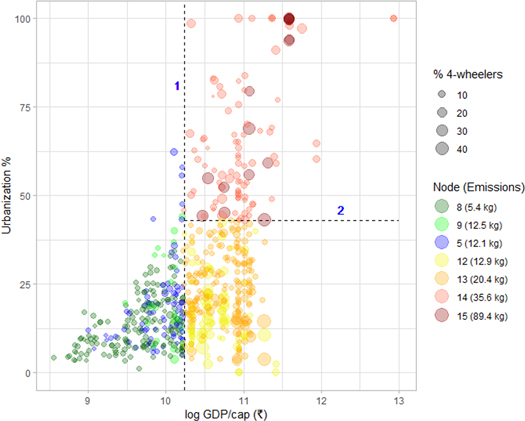
Figure 5. Urbanization and GDP per capita in reference to node levels commuting emissions in India, 2011. Vertical dashed line (1) represents first split by income and horizontal dashed line (2) represents second split by urbanization level in high income districts as a result of tree regressions. Nodes are the same as in figures 2–5.
Download figure:
Standard image High-resolution image
Sixth, among all Indian megacities, Delhi National Capital Region (hereafter Delhi) has the highest commuting emissions per capita (part of node 15). Node 15, which includes Delhi's region, has 2.5 times higher commuting emissions than node 14, which includes most other megacities—Mumbai, Kolkata, Chennai, Bangalore, and Hyderabad. Delhi's higher socio-economic status and heavy reliance on private travel modes (figures 2 and 5) led to higher commuting emissions than in other megacities. This may also be an effect of being the center of government; similarly, as capital of China, Beijing's emissions from car transport exceed those of Shanghai (Liu et al 2007, Creutzig and He 2009). Delhi is also one of the most air-polluted cities in India. This suggests that implementing sustainable transportation options should have higher priority in Delhi than in other megacities.
Seventh, the same district types tend to cluster spatially, as district typology map (figure 3) as well as commuting emissions distribution map (figure S1) reveal. Districts of the same type cluster demonstrates that features covary spatially. The effects is due to underlying drivers vary spatially, e.g. urbanization level. This finding has policy-relevant implication, for instance, adopting strategy from one place to another.
4. Discussion and conclusion
This study provides an improved understanding of commuting emissions in spatial context. To the best of our knowledge, this is the first attempt to assess India's commuting emissions patterns and its drivers at district level (n = 640). Our results provide spatial information relevant to sustainable transport policies at district/regional levels.
Our analysis reveals that GHG emissions from commuting are grounded in urbanization, socio-economic characteristics, and travel mode choices. This result is in accordance with previous research. For instance, previous studies reveal a 1% rise in urbanization increases road transport energy use by 0.37% (Poumanyvong et al 2012) and CO2 emissions by 0.30% (Poumanyvong and Kaneko 2010) in the middle income counries. Similarly, Zhang and Lin (2012) find that in China a 1% increase in urbanization is associated with 0.12% increase in CO2 emissions. Similarly, our estimate reveals that urbanization is positively associated with commuting emissions (urbanization-commuting emission elasticity value is 0.24, that is a 1% increase in urbanization correlates with a 0.24% increase in commuting emissions). The situation in OECD countries is different. For example, Elliott and Clement (2014) showed that per capita CO2 emissions was negatively associated with urbanization and density at county level in USA, after considering constituents of urbanization (i.e. density, percentage of developed land, and urban hierarchy). Urbanization is also associated with denser built-environment, and theory suggests that commuting distances are shorter and more public transit is used, resulting in lower emissions (Fujita 1989, Ahmad et al 2013, Creutzig 2014), in agreement with global data analysis of cities and their energy use and GHG emissions (Marcotullio et al 2013, Creutzig et al 2015, Lohrey and Creutzig 2016). In contrast, our analysis reveals that transport emissions are highest in some of the dense urban areas (figure 4). Districts with similar population density, however, significantly vary in per capita commuting emissions (see node 14 in figure 4). These results indicate that simple-minded densification is an inappropriate policy for reducing commuters' GHG emissions. Instead, a focus on electric two, three, or four-wheeler, and efficient public transit, e.g. in terms of Bus Rapid Transit systems is warranted, like Ahmedabad and Bhopal.
Notably, e-rickshaws are rapidly emerging in metropolitans' suburbs and secondary cities in India, even though they are hardly supported by subsidies (Altenburg et al 2012, Ward and Upadhyay 2018). This suggests that India has the potential to leapfrog oil-driven mobility to electric mobility. Indeed, expansion of e-vehicles would reduce both emissions and air-pollutions, particularly in suburbs and secondary cities (e.g. node 9). However, related infrastructures need appropriate investments for public charging infrastructures in simultaneously and in a coordinated way (Altenburg et al 2012). With such investments, e-vehicle could also become a viable option for long-distance commuting.
Nonetheless, significant variation in commuting emission drivers over space suggests that one-solution fits-all for mitigating transport sector emissions will not work. Solutions instead need to be tailored to geographical contexts (table 2). Finer spatial clustering of determinants of commuting emissions enables both specialization and generalization of policies. Policy interventions can be targeted to the district or region level, acknowledging their different combinations of commuting emission drivers; in turn, policies can also be generalized to similar district/region. Across similar regions, policy makers can learn from context-specific best practice experiences. At a local scale, our analyses enable nuances to be understood by highlighting the spatial heterogeneity of the relationships. For instance, variables' coefficients significantly vary over space (tables S2 and S3). Therefore, a similar change in built environment or mobility-related variables may have different response in mitigating commuting emissions across the country.
Table 2. Summary of district traits and potential interventions by nodes for mitigating commuting emissions.
| Node (Av. Emiss.) | Trait of regiona | Potential interventions |
|---|---|---|
| 8 (5.4 kg) | Low-income, short commuting distance, and less use of three-wheeler | Improving public transport infrastructure |
| 9 (12.5 kg) | Low-income, short commuting distance, but high use three-wheeler | Densification and taxes on fuels |
| 5 (12.1 kg) | Low income, but long commuting distance | Reducing commuting distance (for instance through mixed land use) and improving active/public transport infrastructure |
| 12 (12.9 kg) | High-income, less urbanized with lower road density | Reducing commuting distance, taxes on fuel, and improving active/pulic transport infrastructure |
| 13 (20.4 kg) | High-income, less urbanized but higher road density (e.g. Nellor) | Densification, reducing commuting distance, and improving active transport infrastructure |
| 14 (35.6 kg) | High-income, high-urbanized, with less car use for commuting (e.g. Mumbai) | Reducing commuting distance, and discouraging private transport use, possibly taxes on fuelb |
| 15 (89.4 kg) | High-income, high-urbanized, and high car use for commuting (e.g. Delhi) | Densification, reducing commuting distance, and improving public transport infrastructure, possibly taxes on fuelb |
Note: aSee figure 2 for cut-off line, and figure 3 for geographical location. bHere we suggest fuel taxes based on related study (Ahmad et al 2017).
Another striking example is Delhi's significantly large commuting emissions than other metropolitan cities, associated with high-income, a high share of four-wheeler (node 15). Unlike other districts on the same node, Delhi (and its region) has vast population (over 46 million), and one of the most polluted regions in the world (Ahmad et al 2013). Our analysis suggests immediate policy interventions to mitigate commuting emissions in the region, particularly through alternative commuting modes (non-motorized, e-bikes), also as feeders to improved private transport, as also echoed while studying Delhi's land cover change (Ahmad et al 2016). Rapid action on both demand and supply sides would avoid not only the worst aspects of a collapsing mobility system, but would also support low-carbon trajectories (Creutzig and He 2009, Dhar et al 2018). Delhi, in fact, can emerge as a laboratory for experimenting sustainable options, which may be replicated in other regions.
This study has two limitations: (a) adoption of a modelling approach at district level using aggregated data, whereas microdata (e.g. individual or household) and high spatial resolution (e.g. lower administrative unit than district) could provide a better estimate; (b) census data has home to/from work commuting with travelling modes and distance ranges only. New types of data are necessary to improve these types of studies. For next census, we suggest to collect information on trip lengths and reason and vehicle load factor. Unavailability of India's national travel survey, these additional information could be useful for better assessments.
Our new commuting emissions estimate over space has several implications for urban policymakers. The spatial estimate identifies hotspots for implementing low-carbon commuting options, through restructuring travel characteristics (e.g. travel mode shift, and travel distance) and modifying the built environment (e.g. urbanization, and density aspects). As a result, we gain an improved understanding of the transport sector's mitigation options in spatial context. This will be useful for multi-level of governments to deduce transport policies and programs in local or regional context as per their priorities.
The nonlinear, non-stationarity understanding of India's commuting patterns is scalable also to other issues and other world regions. Our results suggest that policies (e.g. to decrease emissions or improve active transportation) should follow the spatial patterns of the relationships to strengthen their efficiency. Conceptually, our analyses highlights that the study of commuting emissions should be not only socio-economic specific but also location specific. Therefore, we argue for making best use of the increasing availability of big data sources for identifying context-based stratified sustainable solutions.
Acknowledgments
Earlier versions of this article were presented in the Cities and Climate Change Science Conference (Edmonton 2018), Systematizing and upscaling urban solutions for climate change mitigation (SUUCCM) conference (Berlin 2018), and Humboldt-Kolleg 'Sustainable development and climate change: Connecting research, education, policy and practice' (Belgrade 2018). The authors gratefully acknowledge the comments and suggestions received on these occasions. Authors acknowledge Ulf Weddige for excellent data support in the project, and Sumit Mishra for suggesting/providing relevant data and maps. SA is thankful to Jérôme Hilaire, and Max Callaghan for their valuable help in navigating spatial data in ArcGIS/R, Anjali Ramakrishnan for her constructive feedback on an earlier draft, and Vidhi Singh for data assistance. SA acknowledges the Alexander von Humboldt Foundation and the Federal Ministry for Education and Research (Germany) for the research fellowship.