

Abstract
Large missing daytime HONO sources have been reported by many previous studies around the world. Possible HONO sources include ground heterogeneous conversion, aerosol heterogeneous formation, soil emission, and photochemical production. In this study, a consistent 1D framework based on regional and 3D chemical transport models (CTMs) was used to analyze the unknown daytime HONO sources in 14 cases worldwide. We assume that the source of HONO from aerosols is through NO2 hydrolysis (not including its oxidation products) and that non-local mixing effect is negligible. Assuming all the missing unknown HONO source is from the ground, it would imply a NO2-to-HONO ground heterogeneous conversion exceeding 100% in daytime, which is unphysical. In contrast, a strong R2 reaching up to 0.92 is found between the unknown HONO sources and the products of aerosol wet surface area and short-wave radiation. Because the largest unknown daytime HONO sources are found in China due to high concentrations of aerosols and NO2, we derive an optimized NO2 uptake coefficient on the basis of these measurements. The 3D CTM simulations suggest that in some regions of central, eastern, and southwestern (e.g. SiChuan province) China, the aerosol HONO source has the greatest effects on ozone (>10 ppbv) and OH (>200%) in winter. In January, the simulated particulate sulfate level over these three regions increases by 6–10 μg m−3 after including the aerosol-HONO source, which helps reduce the previous model underestimation of sulfate production in winter. Additional measurement studies that target the daytime HONO sources will be essential to a better understanding of the mechanisms and resulting effects on atmospheric oxidants.
Export citation and abstract BibTeX RIS

Original content from this work may be used under the terms of the Creative Commons Attribution 3.0 licence. Any further distribution of this work must maintain attribution to the author(s) and the title of the work, journal citation and DOI.
1. Introduction
Ozone (O3) is one of the most notorious ambient photochemical pollutants worldwide. High concentrations of this pollutant can adversely affect human health and cause substantial reductions in crop yields (Avnery et al 2011, Lu et al 2016). O3 formation is influenced by the photochemical reactions of ROx (OH + HO2 + RO2) and NOx in the atmosphere. Many recent studies have investigated the role of the ROx cycle in O3 formation (Liu et al 2012a, Lu et al 2017). Known atmospheric sources of OH radicals include (but are not limited to) reactions between water vapor and electronically excited oxygen atoms (O1D), the photodissociation of some types of volatile organic compounds (Jaeglé et al 2011), and the photolysis of nitrous acid (HONO) (Liu et al 2012a). According to Lu et al (2017), HONO can contribute to over 30% of the O3 production rate during the daytime at a site of central China in Wuhan City.
Many field campaigns have analyzed the ambient level, diurnal profile, and sources of HONO because of its importance to atmospheric OH radical formation (Su et al 2008, Liu et al 2012a, Lee et al 2016). Short-wave radiation (SWR) induced photolysis has been acknowledged as the major sink of HONO during the daytime. However, the daytime source of HONO remains unknown based on current knowledge and cannot merely be explained by the gaseous reaction between atmospheric NO and OH. As a result, the performance of the 3D chemical transport model (CTM) simulations of OH radicals and O3 might be influenced by the missing HONO source (Zhang et al 2012). Hence, the missing daytime HONO source is highly significant and must be understood to achieve better 3D CTM simulations of O3. Several mechanisms have been proposed to explain the missing daytime HONO source. Su et al (2011) proposed that nitrites in low-pH fertilized soil may be a strong source of ambient HONO (Su et al 2011), whereas VandenBoer et al (2015) reported that surface acid displacement processes were an important potential HONO daytime source in both urban and vegetated regions. Zhou et al (2011) found that surface nitrate loading correlated with HONO flux in a forest environment. Furthermore, in the ambient environment, the heterogeneous conversion of NO2 to HONO on the soot surface was found to increase dramatically in response to solar radiation (Monge et al 2010).
Increasing attention has recently been directed to the heterogeneous conversion of NO2 to HONO on aerosol surfaces. Tong et al (2016) reported that the RH (relative humidity) and PM2.5 (atmospheric particulate matter with a diameter <2.5 mm) concentration might be important factors in the conversion of NO2 to HONO (Tong et al 2016). Combined with 1D model simulation and correlation analysis, Liu et al reported that rapid daytime HONO formation depended on the aerosol surface area and solar radiation strength (Liu et al 2014). They further proposed that dicarboxylic acid anions on the wet aerosol surface could catalyze the enhanced hydrolytic disproportionation of NO2. Given the high levels of discarbonyl compounds and organic acid found in China (Ho et al 2010, Ho et al 2011, Kawamura et al 2013), aerosol might serve a more important role in HONO formation in this region than in other areas of the world. However, the importance of aerosol surface area with respect to heterogeneous HONO formation remains controversial. Some studies reported relatively low (10−7 to 10−6) NO2 uptake coefficients on the aerosol surface area (Stemmler et al 2007), whereas others observed uptake coefficients of 10−4 to 10−3 (Colussi et al 2013).
This study combined observational and 3D CTM simulation data to further investigate the role of aerosol in heterogeneous HONO formation. We applied observational data and output from models to calculate the unknown HONO production source and investigated the relative HONO contributions from aerosol, ground heterogeneous sources and soil emissions. The NO2 uptake coefficient was further estimated based on the calculated unknown HONO source, and the new coefficient was modified into the community multiscale air quality model (CMAQ) to further study the effects of aerosol-generated HONO on O3 concentrations in China.
2. Data and methods
2.1. Observational and model data
In this work, the average diurnal HONO concentrations from 14 different cases worldwide were extracted from the literature to calculate the unknown HONO source. Data from forest or Arctic regions, which have unique underlying surfaces, were excluded. Table 1 lists the locations of the campaigns investigated in this study. In general, the collected HONO data were sampled in China, the United States, Italy, Mexico, and France. The locations of the sampling sites can be found in figure 1 (green triangles). The sampling period as well as the HONO measurement method are listed in table S1 (available online at stacks.iop.org/ERL/13/114002/mmedia).
Table 1. References analyzed for the HONO unknown source in this work.
| No. | References | Location | Time period | Aerosol surface area | Note |
|---|---|---|---|---|---|
| 1 | Liu et al (2014) | Beijing, China | 2007.08 | Observation | Average Case |
| 2 | Liu et al (2014) | Beijing, China | 2007.08 | Observation | Heavy Pollution Case |
| 3 | Hou et al (2016) | Beijing, China | 2014.02/03 | CMAQ a | Clean Case |
| 4 | Hou et al (2016) | Beijing, China | 2014.02 | CMAQ a | Heavy Pollution Case |
| 5 | Zhao et al (2015) | Shanghai, China | 2010.06 | CMAQ | |
| 6 | Yue et al (2015) | Jiangmen, China | 2013.10 | CMAQ a | |
| 7 | Su et al (2008) | Guangzhou, China | 2004.10 | Observation | |
| 8 | Acker et al (2006) | Rome, Italy | 2001.05/06 | GEOS-Chem | |
| 9 | Michoud et al (2014) | Paris, France | 2009.07 | GEOS-Chem a | Summer case |
| 10 | Michoud et al (2014) | Paris, France | 2010.01/02 | GEOS-Chem a | Winter case |
| 11 | Li et al (2010) | Mexico City, Mexico | 2006.03 | GEOS-Chem | |
| 12 | VandenBoer et al (2014) | California, USA | 2010.05/06 | Observation | |
| 13 | VandenBoer et al (2013) | Colorado, USA | 2011.02 | GEOS-Chem | |
| 14 | Gall et al (2016) | Dallas, USA | 2011.06 | Observation |
aThe aerosol wet surface area was corrected by the ratio of the observed PM2.5 concentration over the simulated PM2.5 concentration.
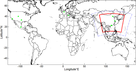
Figure 1. HONO data sampling locations and WRF-CMAQ model domain setting. Green Triangle represents the location of the studied site; blue and red lines represent the domain extents of WRF and CMAQ simulations, respectively.
Download figure:
Standard image High-resolution imageThe wet aerosol surface area was used for correlation analyses (between unknown HONO source) and NO2 uptake coefficient calculations. The observed dry aerosol surface area was corrected using the ratio of the simulated wet surface area over the simulated dry surface area. For some areas with observed PM2.5 concentration data but no available aerosol surface area data, the simulated wet surface area was corrected by the ratio of the observed PM2.5 concentration over the simulated PM2.5 concentration. The availability of the aerosol surface area data for each case is listed in table 1. The wet aerosol surface areas of the sampling sites in China were simulated with the CMAQ model, whereas these surface areas of other sites were simulated using the GEOS-Chem global CTM. Cai et al (2017) reported that the R2 between the active aerosol surface area and PM2.5 mass concentration reached a value of 0.85. Hence, the correction method is adequate for the analysis of correlating the unknown HONO source with aerosol surface area. The random errors in the aerosol surface area corrections will lead to a low bias in the R2 between the unknown HONO source and aerosol surface area.
The OH concentration is needed to calculate HONO production from NO + OH. For study that did not contain OH concentration (e.g. Jiangmen), this value was calculated by the 3D CTM. The J(HONO) values were simulated with CMAQ (within China) and GEOS-Chem (outside China). In addition, SWR(W m−2) data are required for an investigation of the photo-enhanced effect on HONO formation. Because most of the analyzed field campaigns did not report the SWR value, we adopted SWR values from Weather Research Forecast (WRF) corrected by a factor of exp(-AOD) (aerosol optical depth) and from the Modern-Era Retrospective analysis for Research and Applications, Version 2 (MERRA-2) for cases within China and outside China, respectively. We used AOD data from the moderate resolution imaging spectroradiometer (MODIS) AOD 550 nm product. In short, the observation and model data used in this study includes: HONO data, aerosol surface area data, J values (HONO), SWR value (simulated), dry deposition velocities for HONO and NO2 (simulated, section 2.3), and vertical diffusion coefficient (simulated, section 2.3).
2.2. Model configuration
WRF v3.2 was used to simulate the meteorology field for the CMAQ model. WRF has a domain resolution of 27 km, and the domain extent is shown in figure 1 (blue dash line). Final Operational Global Analysis (FNL) Data were used to drive the WRF model. CMAQ (v5.0.1) also has a domain resolution of 27 km, and its domain extent is plotted as a red line in figure 1. The CMAQ domain covers most of China and some neighboring countries, including Korea and Japan. CB05 and ISORROPIA were respectively selected as the gas-phase chemistry scheme and inorganic aerosol scheme for the simulation. The in-line photolysis module, which considers aerosol, ozone, and cloud attenuation effects, was selected for the chemical photolysis rate calculation. The dry deposition velocity in the CMAQ model is calculated using the M3Dry module (Pleim and Byun 2004). The MIX emission inventory was used as the anthropogenic emission input for this simulation (Li et al 2017). More details about the WRF and CMAQ schemes settings have been reported by Lu et al (2015).
GEOS-Chem v10.01 was used in this work. This model was driven by the GEOS-FP met fields and has a worldwide domain extent with a spatial resolution of 2 × 2.5 degree. The GEOS-Chem model is run with full gaseous chemistry and an updated isoprene scheme (Mao et al 2013), and the simulated aerosol species included sulfate, nitrate, ammonium, black carbon (BC), sea salts, natural dust, and primary organic carbon. A non-local scheme (Lin and McElroy 2010) and a relaxed Arakawa-Schubert scheme (Suarez et al 2008) were selected for vertical mixing and convection, respectively, in the simulation. The model-based dry deposition velocity calculation was based on the Wesely resistance-in-series model (Wesely 1989). More details of the dry deposition calculations in GEOS-Chem and CMAQ can be found in the supplemental material.
2.3. Unknown HONO source estimation
We proposed an analytic 1D framework based on the equations shown below to analyze the unknown HONO source. The proposed equations consider the gaseous HONO source (NO + OH), daytime HONO sink, NO2 heterogeneous conversion to HONO from the ground and an unknown source:
where c is the HONO concentration, t is the time, Kz is the vertical eddy diffusion coefficient (table S2), Kc is the HONO chemical reaction coefficient (s−1), F is the vertical HONO flux from the ground and S' is the combination of the unknown HONO source and the source from the reaction of NO and OH (molecule cm−3 s−1). The pseudo-steady state is assumed, ( = 0), and hence we selected for analysis the period when the daytime HONO concentration reached a steady value (the period for each case is listed in table 1). The daytime HONO photochemical lifetime is on the order of 10–20 min. Therefore, when daytime HONO concentrations do not change, it suggests that mixing processes reached a steady state with HONO chemical sources and sinks. We assumed that the unknown HONO source would not change with the height near the surface, allowing us to derive an analytical solution for equation (1):

where X is the observed HONO concentration subtracted the HONO formed by NO + OH. Other unknown gas phase HONO formation reaction is not considered here. Kc is calculated based on the HONO photolysis rate and the reaction rate between HONO and OH, which determine the HONO lifetime during the daytime. F is the net HONO ground flux and is calculated as the upward HONO flux subtracted by the downward HONO flux (dry deposition). S is the unknown HONO source (molecule cm−3 s−1), which is not the ground heterogeneous conversion or the gaseous phase formation. Zhang et al (2016) evaluated several PBL schemes in a 1D column model to investigate the boundary-layer vertical gradients of reactive nitrogen oxides using the DISCOVER-AQ 2011 campaign and reported that the ACM2 scheme is the best and that it can reproduce the profile of the deep turbulent mixing. Hence, in this work, ACM2 scheme was used to calculate the vertical diffusion coefficients for the 1D analytic framework. Non-local mixing is not considered here, which may cause biases in the computed HONO budget calculation. However, the differences among the different WRF boundary layer mixing schemes found by Zhang et al (2016) is considerably less than the uncertainties in unknown HONO aerosols.
In this analytic 1D framework, we assumed that as the NO2 molecules reached the ground via dry deposition, part of them would be converted to HONO and released to the atmosphere immediately (upward HONO flux). According to Liu et al (2014), we assumed that the ground heterogeneous conversion of NO2 and dry deposition of HONO were the major nighttime HONO source and sink, respectively. The NO2 ground conversion ratio (f) during the nighttime could then be calculated by equation (3):

The dry deposition velocities of HONO and NO2 were calculated using the CMAQ (within China) and GEOS-Chem 3D models. The NO2 ground conversion ratio (f) from equation (3) was then used to calculate the upward HONO flux during the daytime. Hence, the F term in equation (2) is calculated by subtracting the right-hand side by the left-hand side of equation (3). The conversion ratio (f) for each case can be found in table S2 in the supplemental material. The parameter, (f), is mainly dependent on the surface characteristics, e.g. surface area, surface type. Hence, it is reasonable to keep the value of (f) constant when the sampling location did not change. Some of other works also applied the dry deposition rate of NO2 to calculate the NO2 ground conversion rate during the nighttime (Li et al 2012, Liu et al 2014).
After acquiring the unknown HONO source S (molecule cm−3 s−1) from equation (1), the NO2 uptake coefficient for aerosol could then be calculated using equations (4) and (5) listed below:


where ka is the first-order NO2 uptake coefficient for aerosol (s−1), Ai and  are the aerosol surface area (μm2 cm−3) and particle radius (μm) for the ith size bin, respectively. ω is the NO2 mean molecular velocity (m s−1), Dg is the gas molecular diffusion coefficient (m2 s−1) and γ is the NO2 uptake coefficient.
We discuss the correlation between the unknown HONO source and aerosol wet surface area in section 3. The NO2 uptake coefficient, calculated using equation (5), was implemented into the CMAQ model and its effects on O3 and OH concentrations in China were investigated.
3. Results and discussion
3.1. Heterogeneous HONO formation from aerosol
The calculated unknown HONO concentration/source and time periods we selected for the study are shown in table 2. The calculated unknown HONO concentrations ranged from 7.17 × 10⁸ (No. 13 for Colorado case) to 4.07 × 10¹⁰ molecules cm−3 (No.2 for 2007 Beijing Heavy Pollution Case), and the unknown HONO sources ranged from 8.70 × 10⁵ (No.13 for Colorado case) to 3.48 × 10⁷ molecules cm−3 s−1 (No.4 for 2014 Beijing Heavy Pollution Case). The calculated unknown HONO concentrations were generally higher in China than in other countries. The unknown HONO sources in Beijing (cases No.1, 2 and 4), Jiangmen (No.6) and Guangzhou (No.7 for Xinken site) all exceeded 107 molecules cm−3 s−1.
Table 2. Calculated unknown HONO concentrations/sources for the selected campaigns.
| Time | Unknown HONO concentrationa | Unknown HONO sourceb | |
|---|---|---|---|
| 1 | 14:00–16:00 | 1.78 × 10¹⁰ | 2.00 × 10⁷ |
| 2 | 15:00–17:00 | 4.07 × 10¹⁰ | 2.84 × 10⁷ |
| 3 | 15:00–16:00 | 1.25 × 10¹⁰ | 9.38 × 10⁶ |
| 4 | 13:00–14:00 | 4.00 × 10¹⁰ | 3.48 × 10⁷ |
| 5 | 14:00–15:00 | 5.76 × 10⁹ | 6.82 × 10⁶ |
| 6 | 10:00–14:00 | 2.39 × 10¹⁰ | 1.70 × 10⁷ |
| 7 | 12:00–14:00 | 1.98 × 10¹⁰ | 2.50 × 10⁷ |
| 8 | 14:00–15:00 | 3.25 × 10⁹ | 6.88 × 10⁶ |
| 9 | 14:00–16:00 | 2.09 × 10⁹ | 3.07 × 10⁶ |
| 10 | 15:00–17:00 | 7.49 × 10⁹ | 1.75 × 10⁶ |
| 11 | 14:00–16:00 | 3.86 × 10⁹ | 4.24 × 10⁶ |
| 12 | 16:00–17:00 | 1.70 × 10⁹ | 1.90 × 10⁶ |
| 13 | 11:00–13:00 | 7.17 × 10⁸ | 8.70 × 10⁵ |
| 14 | 9:00–11:00 | 5.19 × 10⁹ | 7.93 × 10⁶ |
aValues are shown in molecules cm−3. bValues are shown in molecules cm−3 s−1.
Figure 2(a) depicts the R2 between the calculated unknown HONO source and aerosol wet surface area. A total of 14 points were used for the correlation analysis, and each point represents an individual case listed in table 1. The R2 between these two parameters reached 0.87. Some studies have reported that SWR could enhance heterogeneous HONO formation by aerosol (Liu et al 2014, Lu et al 2017). Accordingly, the the R2 value between the unknown HONO source and aerosol wet surface area increased to 0.92 after multiplying by SWR (figure 2(b)). These results provide the evidence to support that the aerosol surfaces comprise an important medium for HONO formation. The OH radical concentrations for Jiangmen (No.6), Shanghai (No.5) and Rome (No.8) cases were calculated by the 3D CTM. A sensitivity test was performed by adding 50% more to the OH concentrations to these three cases and the changes of the calculated unknown HONO source are 2.9% (No.6 for Jiangmen case), 1.5% (No.8 for Rome case) and 3.2% (No.5 for Shanghai case) respectively, when compared to the original values. This shows that HONO production from the reaction of NO + OH is limited when compared to the unknown HONO source and the uncertainty caused by the OH radical computation in these three cases would not influence the results. Since the effect of multiple scattering by aerosols is not included, the attenuation effect of SWR may be overestimated. However, the biases do not lead to false correlations between the unknown HONO source and aerosol since the bias in SWR estimate is monotonic with aerosol AOD.
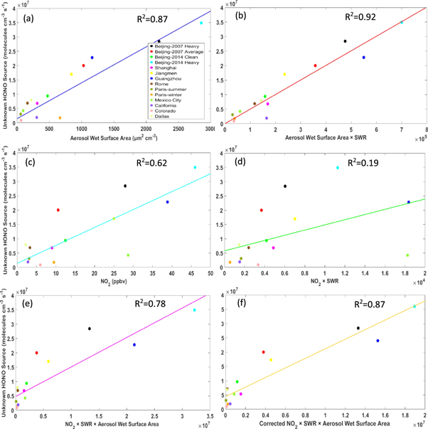
Figure 2. The R2 values of calculated unknown HONO sources with the aerosol wet surface area (a), the aerosol wet surface area × SWR (W m−2) (b), NO2 (c), NO2 × SWR (d), NO2 × SWR × aerosol wet surface area (e) and corrected NO2 × SWR × aerosol wet surface area (f).
Download figure:
Standard image High-resolution imageNO2 is the major gaseous precursor of both HONO and aerosol formation, and this might drive the strong correlation between the aerosol surface area and the unknown HONO source. As shown in figure 2(c), the R2 between NO2 and the unknown HONO source was only 0.62, much lower than the R2 between the unknown HONO source and aerosol wet surface area. Multiplication by SWR decreased the R2 value between the unknown HONO source and NO2 to 0.19. Therefore, figures 2(c) and (d) indicate that the strong R2 between the unknown HONO source and the aerosol surface area was not driven by NO2. However, the R2 between the unknown HONO source and the product of aerosol wet surface area × NO2 × SWR dropped down to 0.78. Except the cases of California, Colorado, Beijing 2007 and Shanghai, the NO2 data in the other datasets were measured by the chemiluminescence method, which might be influenced by the NOy species (e.g. PAN). We further applied the observed seasonal ratios of coincident NO2 measurements of by the chemiluminescence instrument to the more selective photolytic instrument reported by Zhang et al (2018) to correct the NO2 data and found that the R2 (0.87) increased after the correction (figure 2(f)). Xu et al (2013) reported that this ratio varied in different seasons and locations. Hence, the applied correction ratios by Zhang et al (2018) may not be representative for the different campaigns in this study. By using a consistent NO2 dataset, the R2 between the unknown HONO source and the product of SWR × NO2 × aerosol surface area was the highest when compared to other correlations in Liu et al (2014). Therefore, figures 2(e), (f) implies that the decrease of R2 after adding NO2 might be caused by the inconsistent uncertainties in NO2 measurements in different campaigns. The decrease of the R2 value may reflect some of the approximations used in this study. However, we believe that the change may be more numerical than physical. Panel (b) of figure 2 shows much more evenly distributed data points without NO2 than panel (f) with NO2. In panel (f), there are effectively only 7 data points because the low NO2 × SWR × aerosol wet surface area data points are essentially lumped together. The large deviations of the three data points (in red, black, and blue) from the regression line explain most of the decrease of the R2 value. Recent studies pointed towards much faster photolysis of aerosol nitrate as a source of HONO (Ye et al 2016, Ye et al 2017). Our analysis cannot rule out that this pathway contributes significantly to daytime HONO formation. Given the relatively small amount of nitrate in aerosols, the supply of aerosol nitrate through the reaction of OH and NO2 in daytime essentially balances out nitrate photolysis and therefore the production of HONO in aerosols has a similar daytime cycle as OH. Modeling analysis of summer data at Wangdu, China (e.g. Liu et al 2017, Tan et al 2017) suggests that if aerosol nitrate photolysis rate is ten times higher than that of gas-phase HNO3 photolysis, the pathway will provide <10% of the daytime unknown HONO (Hang Qu 2018 personal communication). More research is required to understand if this mechanism can reproduce the observed daytime variation of HONO (Liu et al 2014).
Besides the investigation of the averaged unknown HONO source around the world, the day-to-day unknown HONO source has also been analyzed for the Beijing 2007 case. During the sampling period in this campaign, eleven days' data are available (e.g. valid aerosol surface area data, no precipitation, and at least 2 h stable daytime HONO concentrations). However, the MODIS AOD data are available for only five days and hence, the correlation between the unknown HONO source and aerosol wet surface area × NO2 × SWR was not examined. Shown in figure S1, the unknown HONO source still has a relatively high R2 with the aerosol wet surface area, which demonstrates that aerosol surface is possibly an important driver for the formation of HONO during daytime.
Ground heterogeneous conversion might also be an important potential source of heterogeneous HONO formation. Hence, we investigated whether ground heterogeneous conversion could sustain the daytime HONO level. We excluded the third term in equation (2) and set the unknown HONO as directly equal to the ground-generated HONO. The ground NO2-to-HONO conversion ratio, (f), was then calculated by substituting all other parameters into this modified equation. The new f values for different cases are shown in table 3. Based on our calculation, the NO2-to-HONO conversion ratios of all cases, except Beijing 2007 Heavy Pollution (99%), Mexico City (37%) and Colorado (87%), exceeded 100% if the aerosol heterogeneous formation was not considered. In other words, these results suggest the non-physical conversion of one NO2 molecule to more than one HONO molecule on the ground. This result indicates that NO2 ground heterogeneous conversion cannot be the only major unknown HONO source under most circumstances. We note that it is assumed that soil nitrate is not a source of atmospheric HNO2.
Table 3. NO2-to-HONO ground conversion ratios without consideration of the aerosol source.
| Conversion ratio | |
|---|---|
| 1 | 118% |
| 2 | 99% |
| 3 | 320% |
| 4 | 290% |
| 5 | 232% |
| 6 | 250% |
| 7 | 195% |
| 8 | 208% |
| 9 | 100% |
| 10 | 195% |
| 11 | 37% |
| 12 | 131% |
| 13 | 87% |
| 14 | 450% |
The calculated unknown HONO concentrations at Chinese sites were large and possibly derived from soil emissions. Through laboratory experiments, Oswald et al (2013) found that the ammonia-oxidizing bacteria in soil can directly emit HONO and reported HONO emission flux values from different types of soil. Notably, differences in emission were great, even for the same type of soil, as demonstrated by the >500% difference between two pasture soil samples taken from different locations. Sörgel et al (2015) reported that acidic soil might not promote HONO emission and stated that the mechanisms of soil emission remained under debate. Given this uncertainty, the HONO emission flux for related soil types could not be applied to equation (1) when estimating the exact HONO budget from soil emissions based on current knowledge.
Hence, we discuss herein the relative importance of soil emissions compared to the aerosol heterogeneous source. Among the seven sites in China, the Beijing and Shanghai sites are located in urban areas, far from farmlands, whereas the Guangzhou (No.7 for Xinken site) and Jiangmen (No.6) sites are in rural areas. The urban areas mainly comprise concrete surfaces, with a small proportion of tree and grass coverage. Hence, soil emission is unlikely to be a major HONO source in urban areas. However, it remains interesting to compare the relative amounts of HONO generated by aerosol sources and estimates of soil HONO flux. Because the sites did not have homogeneous land-use types, we calculated the average HONO emission fluxes of pasture, woody savannah, and grassland according to Oswald et al (2013) and added the optimum value (∼5.8 × 10¹⁰ molecules cm−2 s−1 at 25 °C) to the second term of equation (2). The HONO soil emission flux depends on the soil water content and can decrease to zero when the soil water content is near zero or exceeds 40%. For the soil flux, we used the peak value (optimum) for each soil type at an approximate soil water content of 15%. After adding the potential soil emission flux, the ratios of aerosol-generated HONO (the third term in equation (2)) versus observed HONO are 56.5%, 80.5%, 34.1%, 69.9%, 53.2%, and 60.9% for the Beijing 2007 average and heavy cases (No.1 and 2), Beijing 2014 clean and heavy cases (No.3 and 4), Guangzhou (No.7), and Jiangmen cases (No.6), respectively. The optimum soil emission could sustain the daytime HONO budget in the Shanghai case (No.5), for which the aerosol concentration was relatively low. At the optimum HONO soil flux, however, HONO from an aerosol source still accounted for more than 60% of the total HONO budget for both the Beijing heavy pollution cases. This further demonstrates that aerosol is an important HONO source in China in urban sites with high aerosol loading. Earlier soil studies found that N2O correlated positively with soil temperature (Dobbie and Smith 2001, Schindlbacher et al 2004). In a soil model, Parton et al (2001) reported that at temperatures below 10 °C, the parameter used to characterize the nitrification process decreased dramatically. Oswald et al (2013) also showed that the soil HONO emissions would decrease with decreasing temperature. In winter, low soil temperatures prohibit soil HONO emissions, and aerosol becomes a more important medium for heterogeneous HONO formation (e.g. No.4 case).
3.2. NO2 reactive uptake coefficient
As introduced in section 1, the NO2 reactive uptake coefficient can be calculated using equations (4) and (5) once the unknown HONO source has been acquired. Because high daytime HONO sources have been along with high aerosol loading are found in China (table 2), the NO2 reactive uptake coefficients for the first seven cases were calculated and used to study the regional effect on O3 in China (in section 3.3). As shown in table 4, the calculated γ values range from 1.0 × 10⁻⁴ (Beijing 2014 heavy pollution case) to 7.9 × 10⁻⁴ (Shanghai 2010 case). The magnitudes of our calculated γ values are equivalent to those reported by Colussi et al (2013) and those used by Liu et al (2014) and Wong et al (2012) for 1D/3D model simulations. As introduced in section 1, some aerosol components (e.g. dicarboxylic acid anions) can enhance HONO formation. Nie et al (2015) observed a high NO2/HONO ratio in the mixed plumes resulting from biomass burning and fossil fuel emission and concluded that this mixed aerosol could promote HONO formation. Other studies reported that the NO2-to-HONO conversion ratio could be influenced by mineral (e.g. Al2O3) (Romanias et al 2013) and metal (e.g. Fe2+) (Kebede 2015) compositions. According to an observation study, the metal compositions of aerosols in China exhibit large daily variations (Okuda et al 2004). Recently, Han et al (2016 and 2017) reported that the NO2 uptake coefficient and HONO yield would not change with light intensity on the humid acid; however, once the benzophenone was added, the HONO yield increased linearly with the light intensity. Hence, differences in γ values may be attributable to differences in aerosol components during different periods and at various locations. Another factor that influences the uptake coefficient calculation is the interference of the chemiluminescence measurements of NO2 as discussed in section 3.1. More field experiments are needed to verify the dominant factors that affect the magnitude of the reactive NO2 uptake coefficient in an ambient environment.
Table 4. Calculated NO2 reactive uptake coefficients (γ) for the seven cases in China.
| γ | γ/SWR | |
|---|---|---|
| 1 | 7.6 × 10⁻⁴ | 2.2 × 10⁻⁶ |
| 2 | 1.9 × 10⁻⁴ | 8.8 × 10⁻⁷ |
| 3 | 6.2 × 10⁻⁴ | 1.8 × 10⁻⁶ |
| 4 | 1.0 × 10⁻⁴ | 4.2 × 10⁻⁷ |
| 5 | 7.9 × 10⁻⁴ | 1.5 × 10⁻⁶ |
| 6 | 2.3 × 10⁻⁴ | 8.2 × 10⁻⁷ |
| 7 | 2.1 × 10⁻⁴ | 4.5 × 10⁻⁷ |
Liu et al (2014) assumed a linear dependence of γ on SWR. Using their method, we calculated the γ/SWR (γ'), as shown in the second column of table 4. Our γ' values for the seven cases were on the order of 10−7 to 10−6. In some modeling studies, such as that conducted by Zhang et al (2012), the reactive NO2 uptake coefficient was set to equal the magnitude of γ' calculated in this work, without considering the photo-enhancement effect. Using such a parameterization, the NO2 uptake coefficient during daytime could be underestimated (Liu et al 2014). Accordingly, the aerosol contribution to heterogeneous HONO formation is negligible in some 3D modeling studies. Because the exact soil HONO flux could not be identified, the γ' calculated in this work harbors some uncertainty.
3.3. Effect on O3 spatial distribution
The formation of HONO from heterogeneous NO2 conversion on aerosol and ground surfaces was implemented into the CMAQ model. The effects of aerosols on regional-scale ambient HONO, OH and O3 concentrations were also investigated. The following simulations were set for this comparison: (1) HONO formation mechanisms, including gaseous formation in CB05, tailpipe emission (0.8% of total NOx emission), and ground heterogeneous formation (f set as 0.1) and (2) the mechanism listed in the first set of simulations, together with the aerosol heterogeneous HONO formation based on equation (4). We used the same CMAQ domain shown in figure 1 for this sensitivity comparison. January, April, July, and October 2015 were selected for the simulation, representing four different seasons. To determine heterogeneous HONO formation on the aerosol surface, we parameterized the reactive NO2 uptake coefficient by γ = γ' × SWR. As shown in table 4, the γ' value differed for each case. Given the short lifetime of HONO for our analysis periods, HONO sources should be balanced by its chemical loss. We therefore obtain the optimal γ' value by minimizing the squared difference between HONO sources and chemical sink for all data points in table 1. The value of the optimized γ' is 5.0 × 10⁻⁷.
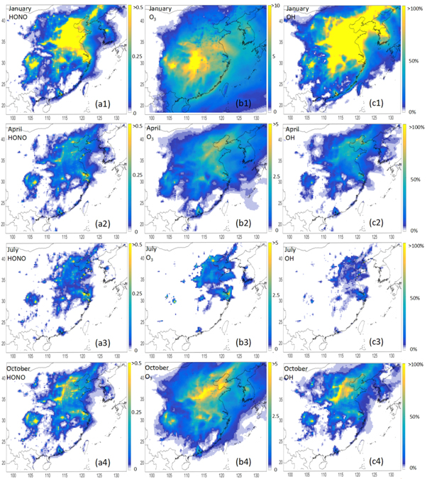
The difference between the CMAQ baseline and updated HONO heterogeneous formation scheme is shown in figure 3. Following the update, during winter daytime (9:00 am–17:00 pm), a simulated HONO difference generally greater than 0.5 ppbv mainly appeared in central, southwestern (SiChuan Basin) and eastern China (Yangtze River Delta). The difference in OH was also centered in this region and reached approximately 200% after updating the scheme. The O3 differences in some of areas of this region reached 10 ppbv. In summer, the differences in HONO, O3, and OH in the northern plain and eastern coast of China were relatively larger than those in other places. The simulated spatial difference in July in this study was similar to that in August as reported by Liu et al (2014). The differences in the spatial patterns of these three species between April (spring) and October (autumn) were similar. In the northern central plain of China, the differences for O3 and HONO were larger during October than during April. When an adequate HONO soil emission module is included, the simulation differences of HONO, O3, OH are expected to become larger.
Figure 3. Monthly average changes in HONO (ppbv), O3(ppbv) and OH (%) levels during 9:00 am–17:00 pm in January, April, July and October 2015 (1–4 represent the cases in different seasons and (a)–(c) represent the changes of HONO, O3 and OH).
Download figure:
Standard image High-resolution image
The simulation over China yielded a much larger difference in winter than in summer, which can be attributed largely to two factors. (1) The aerosol concentration over the northern plain of China is higher in winter than in summer because of weaker, stable meteorology conditions (Zou et al 2017). (2) As noted by Liu et al (2014), the OH source generated by O (1D) + H2O is much smaller in winter than in summer because of the low RH in winter. Accordingly, heterogeneous HONO formation from aerosol plays a more important role with respect to the radical budget and the O3 ambient level during winter. Based on this result, the O3 concentration would decrease if the particulate matter level decreases, especially during winter. However, the O3 production rate would increase as the aerosol optical depth decreases, in contrast to the effect of aerosol on the formation of HONO (Lu et al 2017). The HO2 uptake by aerosol has not yet been included in the CMAQ model. If this mechanism is active, however, the HO2 concentration would increase as the aerosol concentration decreases, which would promote O3 formation (Liu et al 2012a). Hence, in the future, it is important to investigate the combined effects of aerosol on O3 formation in China.
Two important factors are needed in future studies to improve the 3D CTM simulations of the ambient HONO concentrations in China: (1) the effects of aerosol components on the coefficient of NO2 heterogeneous uptake and (2) the important factors determining HONO soil emissions. Liu et al (2012b) investigated satellite products and reported a relatively high concentration of glyoxal (discarboxylic acid precursor) in central China. Colussi et al (2013) reported that the carboxylate anions can work as a catalyst to promote the disproportionation of NO2 on water and HONO formation. This may have driven the heterogeneous HONO generation in the northern central plain of China. Yabushita et al (2009) also reported that the NO2 uptake coefficient can be enhanced by several order of magnitude by the disproportionation of gas phase NO2 on the air/water interface. More experimental studies are needed to quantify the effect of the aerosol component on the production of HONO. Although Oswald et al (2013) reported the HONO emissions of different soil types, large emission differences were observed even for single soil type, and the factors that determine this process will require further identification in the future.
Several recent studies found that current mechanisms in 3D CTMs could not explain the observed sulfate production rates during winter in north and central China (Wang et al 2014, Zheng et al 2015). The following reactions could oxidize sulfur(IV) and produce particulate sulfate (R2–R4 are aqueous phase reactions):


As shown in figure 3, the OH and O3 concentrations increased substantially after the heterogeneous HONO production in January was added. H2O2 would increase as a result of increases in OH and HO2. According to R1–R4, increases in OH and O3 could promote the formation of  which might partly explain the missing sulfate formation in the 3D CTMs. Spatially enhanced sulfate production in January is demonstrated in figure S2 in the supplemental material. Sulfate production increased by approximately 6–8 μg m−3 in the northern central plain and by 10 μg m−3 or more in the Sichuan Basin. Czader et al (2013) noted that the CMAQ underestimated the daytime OH and HO2 concentrations of a polluted air mass. In other words, the missing daytime OH could explain part of the missing particulate sulfate in the 3D CTMs.
3.4. Conclusion
In this study, a consistent 1D framework based on regional and 3D CTMs was used to analyze the unknown daytime HONO sources in 14 cases worldwide. We assume that the source of HONO from aerosols is through NO2 hydrolysis (not including its oxidation products) and that non-local mixing effect is negligible. We found that the daytime unknown HONO source correlated strongly with the aerosol wet surface area. If all unknown HONO were derived from NO2 ground heterogeneous formation, the NO2-to-HONO conversion fraction would exceed 100% in most cases, which is unphysical. After adding the optimized soil emission, heterogeneous HONO formation from aerosol still accounted for more than 60% in the two urban heavy pollution cases. Furthermore, low soil temperatures in winter could prohibit the emission of HONO from soils. Hence, our results indicate that aerosol should play an important role in daytime HONO heterogeneous formation, especially on days affected by heavy pollution and winter temperatures. This result contrasts with the general assumption that aerosols are insignificant with regard to daytime HONO formation. The NO2 uptake coefficient was estimated for seven cases in China, leading us to propose that variations in the uptake coefficients depend on the aerosol composition. According to the CMAQ simulation results, the aerosol generated HONO can contribute up to 10 ppbv of O3 in central China. Further investigations of the effects of different aerosol components on HONO production in China are warranted, because such efforts could improve O3 and PM2.5 simulations based on 3D CTMs.
Acknowledgments
We thank the CalNex 2010 campaign for making the data public. We also thank the constructive comments from the anonymous reviewers. We appreciate the help from Prof Alexis Lau (HKUST) for the CMAQ model consultation. This work was supported by the Research Grants Council of Hong Kong Government (Project No. T24/504/17). Xingcheng Lu was supported by the Overseas Research Award from the Hong Kong University of Science and Technology. Yuhang Wang was supported by the Atmospheric Chemistry Program of the US National Science Foundation.