

Abstract
Since 1992, there has been a revolution in our ability to quantify the land ice contribution to sea level rise using a variety of satellite missions and technologies. Each mission has provided unique, but sometimes conflicting, insights into the mass trends of land ice. Over the last decade, over fifty estimates of land ice trends have been published, providing a confusing and often inconsistent picture. The IPCC Fifth Assessment Report (AR5) attempted to synthesise estimates published up to early 2013. Since then, considerable advances have been made in understanding the origin of the inconsistencies, reducing uncertainties in estimates and extending time series. We assess and synthesise results published, primarily, since the AR5, to produce a consistent estimate of land ice mass trends during the satellite era (1992–2016). We combine observations from multiple missions and approaches including sea level budget analyses. Our resulting synthesis is both consistent and rigorous, drawing on (i) the published literature, (ii) expert assessment of that literature, and (iii) a new analysis of Arctic glacier and ice cap trends combined with statistical modelling.
We present annual and pentad (five-year mean) time series for the East, West Antarctic and Greenland Ice Sheets and glaciers separately and combined. When averaged over pentads, covering the entire period considered, we obtain a monotonic trend in mass contribution to the oceans, increasing from 0.31 ± 0.35 mm of sea level equivalent for 1992–1996 to 1.85 ± 0.13 for 2012–2016. Our integrated land ice trend is lower than many estimates of GRACE-derived ocean mass change for the same periods. This is due, in part, to a smaller estimate for glacier and ice cap mass trends compared to previous assessments. We discuss this, and other likely reasons, for the difference between GRACE ocean mass and land ice trends.
Export citation and abstract BibTeX RIS

Original content from this work may be used under the terms of the Creative Commons Attribution 3.0 licence.
Any further distribution of this work must maintain attribution to the author(s) and the title of the work, journal citation and DOI.
1. Introdution
Permanent ice covers 12.5% of the land surface of the Earth and contains about 70% of the world's freshwater. It comprises the two great ice sheets that cover Antarctica (the AIS) and Greenland (the GrIS) and glaciers and ice caps (GIC). The distinction between these two categories is one of size. Figure 1 shows the geographic distribution of land ice, alongside the area and percentage of glaciers that are marine versus land terminating. Almost all land ice (99.5%) is locked in the ice sheets, with a volume in sea level equivalent (SLE) terms of 7.4 m for Greenland, and 58.3 m for Antarctica, while glaciers is estimated at around 41 cm (Vaughan et al 2013). Thus, the ice sheets are the largest potential source of future sea level rise (SLR) and represent the largest uncertainty in projections of future sea level.
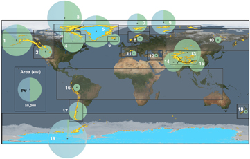
Figure 1. Distribution of land ice over the surface of the Earth. The 19 numbered, yellow shaded areas represent the GIC regions or sectors that are typically chosen for regional mass balance studies of GIC. The blue shading illustrates the ice sheets covering Antarctica and Greenland. The size of the coloured circles indicates the glacierized area for each sector and the green colour is used for the proportion of land-terminating glaciers with blue shading for marine-terminating (Vaughan et al 2013). Section S4.2 of the supplement available at stacks.iop.org/ERL/13/063008/mmedia provides the names of the regions.
Download figure:
Standard image High-resolution imageDespite their diminutive size in comparison to the ice sheets, GIC have dominated the land ice contribution to SLR during the 20th century (Vaughan et al 2013). This has only changed over the last decade due, primarily, to the accelerating contribution of the GrIS since about 1995 (Rignot et al 2011). GIC were the dominant source partly because, on short time scales, they are more sensitive to external forcing compared to the ice sheets. While GIC contain a much smaller reservoir of ice, they are of considerable importance for water resources (Immerzeel et al 2010) and local economies (Huss et al 2017). Changes in downstream discharge rates, glacier extent and exposure of previously pristine permafrost will have important socio-economic consequences.
1.1. The importance of understanding present-day and future land ice trends
Sea level rise is considered to be one of the most serious consequences of future climate change. It is estimated that up to 187 million people could be displaced by a global mean sea level rise of 1 m (Nicholls et al 2011) and the cost of infrastructure damage and land degradation will be immense (Nicholls and Cazenave 2010). The AR5 produced projections for SLR to 2100 for different future climate scenarios. The dominant uncertainty, for high end emission scenarios, in these projections is the potential contribution of land ice (Church et al 2013). Indeed, for the ice sheets, the dynamic contribution (the part due to changes in ice flow rate rather than surface processes) was independent of climate scenario because 'the current state of knowledge does not permit a quantitative assessment', except for the GrIS and the most extreme warming scenario. More recent studies suggest that the potential contribution from Antarctica, in particular, could be larger than forecast in the AR5 (DeConto and Pollard 2016). That study, and many other ice sheet modelling studies, used past behaviour to either calibrate the model or as a target for it (Price et al 2017). Thus, robust and reliable estimates of land ice trends and their relationship to external forcing and internal variability in the climate system, are essential for improved projections of future behaviour. They are also important, as we will explain in section 1.4, for constraining and closing the sea level budget (SLB).
Another important reason for constraining the recent contribution from land ice is in the use of so called Semi-Empirical Models used for SLR projections. These models use the relationship between past changes in SLR and surface air temperature to predict future changes based on climate warming scenarios (Jevrejeva et al 2010, Rahmstorf 2007). There is a lag between a change in temperature and SLR, and there will be multiple lags depending on what part of the climate system is responding: the oceans (via thermal expansion), land hydrology, GIC or the ice sheets. Improved estimates of the land ice response to external forcing and internal variability will, in turn, improve the predictive skill of semi-empirical models. Thus, for a range of reasons, knowledge of past and future mass trends of both GIC and the ice sheets is important. It is worth noting that this has not always been the consensus view. Prior to the advent of high fidelity satellite observations in the 1990s, it was generally believed that the ice sheets responded slowly (over millennia) to external forcing and required a large amplitude perturbation to demonstrate a significant response (Vaughan 2008).

Figure 2. Schematic representation of the marine-terminating portion of an ice sheet or glacier with bedrock below sea level.
Download figure:
Standard image High-resolution image1.2. Mass balance of GIC and ice sheets
The mass balance of a glacier or an ice sheet represents the trade-off between gains, primarily through snowfall, and losses, through melting at the upper surface (also called surface ablation), iceberg calving (in the case of marine-terminating land ice), bottom melting underneath floating ice shelves and basal melting at the ice/bedrock interface, which is generally a small term. Snowfall and surface ablation are the key terms that make up the surface mass balance (SMB). Calving and bottom melting (beneath floating ice shelves) can be aggregated into a single term, which is the ice discharge (D) across the grounding line (figure 2). If the SMB equals D, then the ice mass is in balance: the net accumulation of ice at the surface is balanced by discharge across the grounding line, assuming that basal melt beneath the grounded ice is negligible. This does not, however, necessarily mean that the ice mass is in equilibrium as we shall discuss in section 1.6.
For land terminating glaciers, such as those in Asia and the European Alps, only surface melting is important as D is zero (there is no grounding line flux). In the case of marine-terminating glaciers, such as those in most of the Arctic (see figure 1), discharge is an important, and sometimes dominant, component of mass loss. For Antarctica, surface melting is negligible because air temperatures, even in summer, are generally below freezing and it is a reasonable approximation to assume that all mass is lost through discharge across the grounding line (see box 1). For Greenland, about 60% of the present-day mass removal is from ice discharge, and 40% from surface ablation but their influence on recent imbalance is the other way around (van den Broeke et al 2009, van den Broeke et al 2016). In other words, the change in surface processes has been responsible for 60% of the imbalance and change in D for 40%.
Box 1. Jargon box/primer.
| Altimetry: Satellite radar (ERS-1, ENVISat, CryoSat 2) and laser (ICESat) altimetry can be used to measure, with high accuracy, the changing surface elevation (and hence volume) of an ice sheet or ice cap and, in the case of ICESat, larger glaciers. To go from a volume change (∆V) to a mass change (∆M) requires knowledge of the density of the medium that has changed. Over polar ice masses, this may be that of the surface layer (called firn), which can have a density of 350 kg m−3 or that of ice, with a density of 918 kg m−3. Clearly, the difference between these two results in a concomitant difference in the inferred mass trend. Knowing what density to use requires knowledge about the process driving the volume change: is it due to surface processes such as changes in snowfall and runoff, or is it due to a change in ice motion (usually termed ice dynamics). In general, it is some combination of the two resulting in the effective density of the volume change having an intermediate value. In addition, the rate of densification from firn to ice depends on temperature and accumulation rate. A change in either of these can affect, what is called, the firn compaction rate, and hence surface elevation without having any change in mass. Over sub-polar glaciers these issues are of less significance because the surface firn layer is thinner and closer in density to that of ice. |
| GRACE: The Gravity Recovery and Climate Experiment was launched in 2002 and comprised two satellites flying in tandem at about 200 km separation (Tapley et al 2004). They measure changes in the gravity field at the Earth's surface and below it within the mantle. From these gravity anomalies, it is possible to infer a mass change. The effective resolution of GRACE is about 300 km so it cannot measure changes of individual glaciers or ice caps but integrates the changes over larger areas. To determine ice mass trends from GRACE, it is necessary to remove any signals from other sources of mass movement. These are primarily due to land hydrology and a process called glacial isostatic adjustment (GIA). |
| Glacial isostatic adjustment (GIA): GIA is the solid Earth response to past loading of the lithosphere by ice sheets during the last glacial period which ended about 12,000 years BP. Removal of the ice results in uplift of the land and redistribution of the mantle at depth. It makes an important contribution to contemporary sea level changes at a regional scale but also directly affects the gravity anomaly measured by GRACE. Models of the response of the Earth to this loading can be used to predict present-day GIA (Peltier 2004), or it can be reconstructed using a data inversion approach (Wu et al 2010). |
| Grounding line: when a glacier or ice mass is in direct contact with the ocean, there will be a triple junction formed of sea water, bedrock and ice (figure 2). This junction is called the grounding line and is important for several reasons. First, it forms the point at which ice is no longer on land but has become part of the ocean system. At some distance (typically a few kilometres downstream) the ice is freely floating on the ocean (it is in hydrostatic equilibrium) and has almost no influence on sea level anymore. Second, the grounding line is the first point at which the ocean can influence ice mass. Warm ocean water in the vicinity of the grounding line can cause high melt rates (Rignot 1996) and changes in water temperature can directly influence the inland ice speed and discharge into the ocean (Holland et al 2008). Third, under certain circumstances the position of the grounding line can be inherently unstable and small changes in, for example, ocean temperatures, can result in a rapid retreat of the grounding line and, as a consequence, ice mass loss (Schoof 2007). |
Both Greenland and Antarctica contain GIC around the margins of the main ice sheets (regions 5 and 19 in figure 1), often referred to as peripheral GIC (PGIC). Some studies consider the mass balance of the ice sheets and the PGIC separately but there has been, in general, no consistency in the treatment of PGIC and many studies do not specify if they are included or excluded from the total. For Greenland, the PGIC are a significant proportion of the total mass imbalance (circa 15%–20%) (Bolch et al 2013). The GRACE satellites have an approximate spatial resolution of 300 km and the large number of studies that use GRACE, by default, include all land ice within the domain of interest. For this reason, in the following sections, when discussing AIS or GrIS mass trends, the values include PGIC. To avoid double counting PGIC in estimates of GIC, such as modelling studies, that include these regions, we have subtracted the best estimates for PGIC contribution from the total GIC value. However, it is not always possible to determine what the GIC estimate refers to (Yi et al 2015), most likely because the authors are not aware of the difference. In general, where a study has used GRACE to determine the GIC trend, we assume that this does not include PGIC as this will be part of the ice sheet estimates.
The AIS is usually partitioned into the West (WAIS) and East (EAIS) separated by the natural geographic barrier of the Transantarctic Mountains. Other factors, however, also differentiate the two. The WAIS is a predominantly marine ice sheet—one that is resting on bedrock below sea level—on a retrograde bed slope (where the bed deepens inland). This configuration is believed to be inherently unstable and is associated with the marine ice sheet instability hypothesis first posited in the 1970s (Hughes 1973, Mercer 1978) and now, potentially, already underway (Joughin et al 2014). The Antarctic Peninsula, often considered part of the WAIS, but geographically and climatologically distinct from it, also has regions that satisfy the marine instability criteria (Bamber et al 2009). It is a region that, until recently, has experienced a marked warming and dramatic changes to a number of fringing ice shelves, with associated changes to grounded ice motion (Rignot et al 2004, Rott et al 1998, Scambos et al 2014, van den Broeke 2005, Vaughan and Doake 1996). More recently accelerated mass loss has also been identified for the southern Peninsula (Wouters et al 2015). In contrast, the EAIS is predominantly resting on bedrock above sea level although some sectors are marine with limited areas of retrograde bed slopes (Bamber et al 2009) and have shown recent signs of dynamic change (Greenbaum et al 2015). It is, therefore, believed to be, largely, more stable than its western neighbour and recent observations tend to support this view (Martín-Español et al 2016a), although paleo-proxy data suggests variability in ice extent for part of East Antarctica during previous warm epochs (Gulick et al 2017).
1.3. How mass balance is determined
There are three main methods for estimating or measuring the mass balance of an ice mass, each of which relies on different types of satellite instrument, based on observations (but, typically, including model output to address one or more unobserved processes).
The first method involves measuring changes in elevation of the ice surface over time either from imagery or from altimetry (see box 1). Radar and laser altimeters have been flown on both satellite and airborne platforms and all have been used to make repeat measurements of elevation change over both GIC and the ice sheets (Arendt et al 2008, Helm et al 2014, Krabill et al 2000). ERS-1 was launched in 1991 and was the first satellite to carry a radar altimeter that covered a substantial proportion of both the GrIS and AIS. It had a latitudinal limit of 81.5° which meant it covered almost all of the GrIS and four-fifths of the AIS (Bamber and Kwok 2003). It was succeeded by ERS-2 in 1995, ENVISat in 2000 and CryoSat-2 in 2010, which extended the latitudinal limit to 88°. Autonomous satellite laser altimeter observations over the same area were provided from 2003–2009 by ICESat.
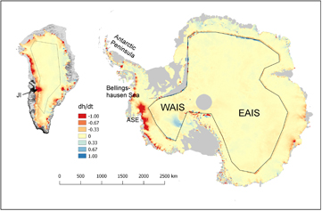
Figure 3. Mean elevation rates for 2010–2017 for the Antarctic and Greenland Ice Sheets, derived from CryoSat-2 radar altimetry (updated from Hurkmans et al (2014) and Martín-Español et al (2016a)). Both ice sheets are shown at the same scale. Regions of mass loss, concentrated around the southeast and western margins of the GrIS and the Amundsen sea Embayment (ASE) of the WAIS, are shown in red. The solid black polygons show where CryoSat- 2 switches between different modes, which introduces some artefacts in dh/dt near the boundary between them.
Download figure:
Standard image High-resolution imageThis first method involves interpolating a heterogeneous distribution of elevation differences (dh/dt) into a volume change and from volume to mass (dm/dt), requiring knowledge of the density of the volume change (Sørensen et al 2011). For GIC, it is usually assumed that this is the density of ice but for the ice sheets this is not the case as the upper layer is compacted snow known as firn, which can have a density around 2.5 times smaller than ice (see box 1). Changes in firn compaction rate can alter the ice sheet volume without any change to its mass (Sørensen et al 2011). Although, GIC, and in particular Arctic ice caps, can have an extensive firn layer, it is roughly an order of magnitude less deep compared to the interior of the ice sheets and, as a consequence, generally has less impact on volume changes. Figure 3 illustrates the mean elevation trends for 2010–2017 for the GrIS and AIS, obtained from CryoSat-2 radar altimeter data. It shows the sectors of both ice sheets that have been the primary contributors to SLR during the satellite era, as these same regions have dominated mass loss over most of the period from 1992–2016. In the interior of both ice sheets, the elevation rates are small and close to the signal threshold for detecting a mass change from volume change estimates. This is discussed in more detail in section 2.1 on the EAIS.
For glaciers, mass balance can also be measured via direct, field-based, observations although these only exist for a small proportion (<200) of the >200 000 glaciers that have been identified (Zemp et al 2009). Attempts have been made to extrapolate these in-situ data to cover all glacier sectors shown in figure 1 (Cogley 2009, Dyurgerov and Meier 1997), but because of the non-uniform sampling in altitude, aspect, climatic setting and size of the field-based data, scaling up to entire mountain ranges/sectors introduces large uncertainties (Gardner et al 2013). In general, the agreement between scaling up of these direct observations and other estimates, both regional and global, has been mixed (Gardner et al 2013). Length and volume change records extend back over a century for some glaciers and these can be used to calibrate glacier mass balance models that are driven by global climatologies such as surface air temperature data (Marzeion et al 2015) and re-analysis products (Radic and Hock 2010, Radić et al 2014). This approach differs from using a regional climate model (RCM) to estimate, directly, the surface mass balance of an ice mass, as it is based on a statistical scaling relationship. We term this method statistical modelling (e.g. Marzeion et al 2015, Radić et al 2014). While RCMs work well for larger ice masses, such as the ice sheets and Arctic ice caps, the complex topography, and corresponding micro-climatological effects this creates, makes them less suitable for GIC on a smaller scale and/or in mountainous terrain.
More recently, airborne and satellite-based stereo photogrammetry has been used to estimate volume changes of some of the glaciated regions shown in figure 1. With the aid of historical photo archives, this has provided observational reconstructions extending as far back as the 1930s for some sectors (Bjørk et al 2012, Nuth et al 2010).

Figure 4. Comparison of cumulative mass balance trends for the Greenland Ice Sheet and peripheral glaciers and ice caps for 1992–2016, based on satellite altimetry, the input/output method (IOM) and GRACE.
Download figure:
Standard image High-resolution imageThe second method for estimating mass balance is known as the mass budget or Input-Output Method (IOM) and, as the name suggests, involves estimating the difference between the surface mass balance (SMB) and ice discharge (D). The former is comprised of primarily snowfall minus runoff (surface ablation) and, for large ice masses, is often estimated from regional climate models (RCMs) that are forced at their boundaries by re-analyses (Fettweis 2007, Lenaerts et al 2012). The RCMs are coupled to snow diagenesis models so that they can realistically reproduce both atmospheric conditions and processes at and within the snowpack. Discharge comprises ice velocity multiplied by ice thickness across a gate, usually taken to be the grounding line or a short distance inland from it (Rignot et al 2008a, Rignot et al 2008b). As mentioned previously, for land-terminating ice masses D is zero and it is only SMB that determines the state of the ice mass. As will be shown later, when discussing Arctic ice caps, RCMs are of sufficient resolution and sophistication that they can reliably reproduce mass trends without the use of in-situ data.
The third and final approach, and the most recently developed, only became viable with the launch of the Gravity Recovery and Climate Experiment (GRACE) satellites in 2002 (see box 1). They have provided gravity anomaly measurements continuously from 2002 until September 2017 when one of the satellites failed. The gravity anomalies provide information about redistribution of mass at, and below, the surface of the Earth at relatively coarse resolution of about 300 km (see box 1).
The most appropriate approach depends on the location and size of the ice mass. For example, satellite radar altimetry is compromised in areas of high relief such as mountain ranges, while GRACE integrates changes in the gravity field over a characteristic length scale of about 300 km. As a consequence, GRACE cannot provide trends for single glaciers but rather over larger areas such as the whole Svalbard archipelago or basins of the ice sheets (e.g. Jacob et al 2012). Another limitation of using GRACE data to determine mass balance for land-locked GIC is if the redistribution of mass from a glacier to an aquifer is local (within the resolution of GRACE), then the satellites will not see a significant change in gravity even though the glacier imbalance may be large and, in principle, measurable by GRACE. Another constraint is local tectonics, which can affect the solid-earth gravity anomalies in areas of seismic activity (Jacob et al 2012). For example, for High Mountain Asia (HMA; regions 13–15 in figure 1), the uncertainties due to land hydrology and solid-Earth processes are larger than the signal, which is also the case for several other smaller mountain ranges (Jacob et al 2012).
Ice sheet wide agreement between the three approaches has been previously demonstrated for Greenland by Sasgen et al (2012) for the period 2003–2011, although there was less consistency at a basin scale. In figure 4 we present a similar, but longer, time series based on methods published elsewhere (Hurkmans et al 2014, van den Broeke et al 2009, van den Broeke et al 2016, Wouters et al 2013). The results extend the analysis of Sasgen et al (2012), using CryoSat-2 altimetry data, updated RCM simulations downscaled to 1 km (Noël et al 2016) and a GRACE inversion approach (Wouters et al 2008). Excellent agreement is seen between the methods, including for the exceptional melt event in 2012, which has the potential to bias altimeter-derived mass changes estimates (Nilsson et al 2015). It is also apparent the trends from satellite altimetry (in this instance ERS-2, ENVISat, ICESat I and CryoSat-2) are smooth in time and do not capture sub-annual behaviour before 2003. This is because, to achieve adequate sampling in space, it was necessary to average a large number of individual dh/dt estimates and to interpolate to unobserved sectors, especially, prior to CryoSat-2 (Hurkmans et al 2014).
Prior to 2003, we are reliant on satellite radar altimetry (Hurkmans et al 2014) and IOM (van den Broeke et al 2016) alone and it is apparent that there is greater divergence between these two approaches for this epoch (for example from 1995–1998). Observed discharge estimates were used from 2000 onward and are assumed to decrease linearly to 1996 and to be stationary before that (van den Broeke et al 2016). Radar altimetry does not fully sample coastal thinning and requires interpolation to capture the high rates near the margins (e.g. Hurkmans et al 2014). An approach called kriging with external drift was used, which was effective in determining the rates but with a potential delayed signal (by 1–2 years) due to the time it takes for thinning at the margin to propagate sufficiently far inland to be observed by radar altimetry (Hurkmans et al 2014). Thus, our understanding of ice mass changes prior to 2003 is more uncertain.
A promising approach that attempts to address these limitations is to combine GRACE with other gravity data derived from satellite laser ranging (Talpe et al 2017). The advantage of this approach is that it is a more direct measurement of mass movement at the surface with data extending as far back as 1976. The disadvantage is its low spatial resolution and the subsequent challenges in separating mass-movement signals from different sources and processes and the comparatively large errors (Talpe et al 2017). Using this approach, the total error estimate for the GrIS is between 150 and 200 Gt yr−1 and for the AIS around 100–120 Gt yr−1 (Talpe et al 2017).
1.4. The sea level budget and role of land ice
The SLB is relevant with respect to land ice for two interlinked reasons. The first is the central role land ice contributes towards it and the second is that estimates of the SLB can be compared with independent assessments of the land ice contribution. For example, GRACE can measure the global change in mass of the oceans, which should equal the total contribution from land ice along with some other smaller contributions.
Changes in global mean sea level (∆GMSLTotal) is influenced by a number of geophysical processes defined in equation (1), which is commonly termed the SLB:
Where ∆GMSLsteric is the term related to changes in density caused by temperature (thermosteric) and salinity (halosteric) variations, ∆GMSLmass is the term due to mass exchange between the land and ocean and ∆GMSLVLM is the term related to changes in ocean basin volume due to vertical land motion (VLM). The mass term (∆GMSLmass) can be further broken down to include the different land ice components (the focus of this paper):
Where ∆MGIC, ∆MGrIS and ∆MAIS are the change in mass due to glaciers and ice caps, Greenland and Antarctica, respectively. ∆MLWS is land water storage including both natural and anthropogenic factors such as secular trends in precipitation minus evaporation, water impoundment and extraction. ∆Mother captures several other smaller contributions including secular trends in atmospheric water vapour loading and seasonal snow cover.
Since 1992 we have had a reliable record of ∆GMSLTotal for the oceans up to a latitude of ±60° from satellite radar altimetry. In principle, ∆GMSLTotal as measured by altimetry should equal the sum of the three terms on the right-hand side of equation (1), which is termed closing the SLB. Various attempts to close the SLB have been made with considerable progress being made after the launch of the GRACE satellites in March 2002. GRACE allowed, for the first time, a direct measurement of changes in ocean mass and exchange with land. This roughly coincided with a step change in observations of ∆GMSLsteric from the network of Argo buoys that was near-complete by 2005 (Freeland and Cummins 2005, Riser et al 2016). These buoys measure temperature and salinity variations down to a depth of 2000 m and provide the most complete observational record of steric changes in the upper ocean. Vertical land motion is a relatively small term in the range 0.2–0.4 mm yr−1 (Spada 2017, Tamisiea 2011) due, predominantly, to glacial isostatic adjustment (GIA) (see box 1) with an uncertainty of about 0.2 mm yr−1. Thus for 2003 to the present, each term in equation (1) is relatively well constrained. There are, however, other terms related to vertical land motion, as a result of present-day mass exchange that have, in general, been ignored in SLB studies (Frederikse et al 2017, Lickley et al 2018).
For the prior epoch (1993–2003), the steric and mass terms are less well constrained by observations and drift in the altimeter instrument electronics (specifically Topex A from 1993–1998) has also impacted the reliability of the ∆GMSLTotal observations (Watson et al 2015). Despite these limitations, Dieng et al (2017) investigated the SLB for the satellite era (1993–2015) by comparing multiple estimates of each term in equation (1), including the integrated ocean mass trend from GRACE versus the sum of each contribution to this term, namely GIC, Greenland, Antarctica, land water storage, snow storage and atmospheric water vapour changes. The residual difference between the left-hand and right-hand side of equation (1) was found to be 0.0 ± 0.22 mm yr−1 (Dieng et al 2017). This provides, in principle, some confidence in the individual component estimates. However, other studies have obtained both higher and lower estimates of the various components that make up the mass term in equation (1) (section 3.1). Indeed, the uncertainty in the solid Earth influence due to GIA on the GRACE estimate of ocean mass is ±0.5 mm yr−1 alone (Tamisiea 2011). Thus, choices made in the estimates used, and corrections applied, can result in an apparent closure of the budget. We will return to the SLB later in this review, when assessing the veracity of mass trend estimates for the ice sheets and GIC. What the SLB does provide are bounding limits for ∆GMSLmass given estimates of the other terms from recent observations.
1.5. The difference between mass balance and sea level contribution
Understanding of the global land ice contribution to sea level rise is complicated by the fact that ice mass balance and sea level contribution are not the same quantity. In the case of an ice mass with a marine-terminating margin and bedrock elevation below mean sea level, some proportion of the volume of ice lost is below mean sea level. Figure 2 illustrates the typical geometry of most of the WAIS, parts of the EAIS, GrIS and many marine-terminating glaciers in the Arctic. Seaward of the grounding line, the floating ice shelf is in hydrostatic equilibrium with the ocean. If it melts, it has a negligible impact on sea level (there is a small halosteric effect due to dilution of the ocean by freshwater). A change in mass on the landward side, however, does have a direct impact. The grounding line represents, therefore, a natural and logical boundary for defining the mass balance of a marine-terminating glacier/ice mass.
There is a further complication to this apparently simple situation. Imagine a scenario (as is the case for parts of the WAIS) where the grounding line is migrating inland. The change in mass of the grounded ice sheet is the integral of the total ice thickness along the grounding line multiplied by the distance it has moved inland. Consider a 20 km wide glacier (similar to Pine Island Glacier, WAIS) and ice thickness at the grounding line of 1 km. For a grounding line migration rate of 1 km yr−1, the mass loss is 20 km3 yr−1. This is, however, not the same as the SLE contribution, as that comes only from the proportion of ice above buoyancy (tens to over a hundred metres above the black dashed line in figure 2). Typically, grounding lines of fast moving outlet glaciers are close to flotation and this means that the SLE contribution is an order of magnitude smaller than the total mass imbalance. This only matters where the grounding line is moving, which is relevant primarily for parts of the WAIS. However, previous studies of the WAIS have not been clear on whether it is the SLE or the mass imbalance they are estimating when using altimetry and/or IOM (e.g. Rignot et al 2011, Shepherd et al 2012, Sutterley et al 2014). GRACE measurements only detect the SLE contribution and do not measure mass imbalance. Volume change and IOM estimates may do either depending on whether they account for grounding line migration in their calculations. If they do not, then they may be measuring a volume change over floating ice. If they do, then they must estimate the proportion of ice above floatation and discount the remainder if it is the SLE contribution that is being estimated. Later, we investigate the impact of this effect on SLE and mass balance estimate for the WAIS and show that the error is significant if ignored.
For GIC, there may also be a difference between ice mass balance and sea level contribution due to the fact that the meltwater from land-locked GIC may never reach the ocean (Brun et al 2017). For example, in HMA (regions 13–15 in figure 1), it is likely that some proportion of the glacial meltwater is taken up by aquifer recharge, irrigation or other forms of impoundment, particularly for endorheic (or closed) drainage basins (Brun et al 2017).
1.6. The 20th century sea level contribution from land ice
As land ice has a relatively slow response time to external forcing, it is useful to consider its longer-term behaviour, prior to the satellite era. There are, however, limited observational data on the 20th century behaviour of land ice, especially for the ice sheets. The last IPCC report (the AR5) considered whether, modelling and observational data could be used to close the SLB for 1900–1990 (Church et al 2013). Ice sheets were excluded from this assessment, due to lack of reliable estimates. Observations from a small number of in-situ mass balance measurements of individual glaciers (outside of the ice sheets) and upscaling to the 19 regions shown in figure 1 gave a rate of 0.54 ± 0.7 mm yr−1, while statistical modelling produced a slightly higher rate of 0.63 ± 0.28 mm yr−1. Taking into account the other terms in equation (1) (thermal expansion and land hydrology) they obtained a residual (i.e. difference from sea level rise observed by tide gauges) of 0.5 mm yr−1, with an uncertainty range of 0.1 to 1.0 mm yr−1. This could be accounted for by contributions from the GrIS and AIS, but in what proportion was largely unknown.
Since then, two notable advances have been made that help resolve the ice sheet contribution during the 20th century. First, reassessment of the long-term tide gauge record, used to reconstruct SLR, suggests that the 20th century rate has likely been overestimated by 0.3–0.4 mm yr−1 (Dangendorf et al 2017, Hay et al 2015). Second, a reconstruction of the Little Ice Age volume of the GrIS from aerial stereo photogrammetry has provided the first robust estimate of the 20th century contribution from this source (Kjeldsen et al 2015). While the estimate lacks temporal fidelity, it does provide a mean rate of mass loss equivalent to 0.21 ± 0.08 mm yr−1 for the period 1900–1983, with a similar rate for 1983–2003 (Kjeldsen et al 2015).
Combining these two advances with the remaining terms in the SLB provides a constraint on the AIS contribution. Using the value for SLR of 1.2 ± 0.2 mm yr−1 for 1901–1990 (Hay et al 2015), the new GrIS estimate reduces the residual in the AR5 SLB to 0.1 mm yr−1 (−0.4 to 0.5). Although the combined uncertainties are large, this suggests that the AIS was likely close to balance up to 1990. To date, there are, unfortunately, few other approaches available to constrain the behaviour of the AIS prior to the satellite era. The ice sheet has an area of about 13 million km2, larger than the conterminous USA and the only reliable way to make direct, continent-wide observations is, as a consequence, using Earth observation (EO) techniques.
It is also worth noting that, although the SLB approach suggests a near balance for the AIS, it provides no information about regional variations and, by inference, if the ice sheet is in equilibrium. For example, estimates for about the last decade indicate that mass loss from the WAIS has been partly compensated for by gains from the EAIS (Martín-Español et al 2016a). Furthermore, velocities derived from satellite imagery suggest that mass loss for part of the Amundsen Sea Embayment of West Antarctica began as early as the 1970s (Rignot 2008). It is possible, therefore, that recent regional trends (i.e. gains over the EAIS and losses in the WAIS) may have existed for decades prior to our ability to detect them. In terms of the ice sheet contribution to SLR, this may not appear relevant, but it is critical for understanding the evolution of the trends, their origin and drivers, and therefore for predicting their future behaviour. The origins of the losses/gains are also likely different: one due to changes in the ocean and the other, potentially, due to changes in the atmosphere. Likewise in the case of the GrIS, it has been assumed that the ice sheet was close to balance from about 1960 to 1990 (van den Broeke et al 2009). This may be a reasonable assumption, but examination of the longer term (20th century) reconstruction of the SMB over the ice sheet indicates that this was a period of slight cooling with lower ablation and higher snowfall resulting in a more positive SMB (Fettweis et al 2017) that likely compensated the long-term negative dynamic response of the ice sheet to the end of the Little Ice Age (Kjeldsen et al 2015). These two examples highlight the importance of constraining not just the overall balance but the origin of the losses and gains and how they relate to external forcing.
GIC are considerably smaller than the ice sheets. Their individual mass balance can often, therefore, be derived from in-situ observations, but due to the large number of glaciers (about 200 000 are included in the Randolph glacier inventory (Pfeffer et al 2014), the sampling of directly observed glaciers is necessarily sparse. The EO techniques applicable to the ice sheets can, in principle, be applied to GIC, but the small size of individual GIC and their location in often complex terrain reduces the ability of these approaches to provide reliable data with a useful signal to noise ratio. In the first half of the 20th century, glacier length records (Leclercq et al 2014) provide the only direct observations of GIC change that allow for a global assessment of their contribution to sea-level change. These length-change records indicate that glacier retreat, and thus presumable glacier mass loss, started on the global scale around 1850, at the end of the Little Ice Age (Leclercq et al 2011). Glacier statistical modelling, using climate observations as forcing, corroborates the finding that mass loss rates from GIC increased slightly until the 1930s or 1940s, peaking around 1 mm SLE/yr (but with large associated uncertainties), before decreasing until the 1960s or 1970s to around 0.5 mm SLE/yr. The subsequent increase of mass loss rates until present day is apparent in estimates based on glacier length retreat, direct and geodetic observations, and GIC statistical modelling alike (Marzeion et al 2015).
2. Synthesis of mass balance assessments
During the satellite era, and particularly since 2002, there has been an unprecedented increase in the number of studies investigating land ice mass trends. The IPCC AR5 provided a thorough and careful synthesis of those studies published up to early 2013. In preparation for the AR5, two studies were undertaken to attempt to provide so called reconciled estimates of mass trends for the ice sheets (Shepherd et al 2012) and GIC (Gardner et al 2013). In both studies, estimates from the various approaches available (dh/dt, IOM, GRACE and extrapolation of terrestrial data) were compared, and for GIC, combined. Consistency between methods was improved by, for example, focusing on a common time period and common drainage basin definitions and/or areal extent of glaciated land yet inconsistencies remained between published results for specific regions (Gardner et al 2013) or ice sheet sectors and methods. To describe these studies as reconciled is, therefore, not entirely accurate but more a shorthand for a reduction in the inconsistency between results. Since then, new estimates for both GIC regions and the ice sheets have been published, which further explore or challenge the consistency (or lack thereof) between methods and approaches.
Here, we focus primarily on studies published since the AR5 to: (i) present and update ice sheet trends for GrIS and AIS to 2016 based on previously published results; (ii) present a new synthesis of GIC trends by combining the latest satellite observations and statistical modelling; and (iii) assess the consistency between land ice mass loss and the global SLB. The outcome is a comprehensive, consistent and rigorous assessment of the land ice contribution to SLR from 1992–2016.
A complete list of previously published results considered in this review are provided in tables S1 (AIS), S3 (GrIS) and S5 (GIC) in the supplementary data. In our assessment of consistency between the various results, we have used a new approach for presenting time-averaged trends. Typically, results have been compared by plotting mass balance values as boxes where the width is the time span and the height is the uncertainty (e.g. Hanna et al 2013). As an increasing number of results are plotted, this becomes harder to interpret, and is also misleading because, in general, each box does not reflect a stationary value in time but plotting it this way tends to make it appear so.
This final point is important as many studies have published a mean rate over a given time period based on the data available, which varies substantially between methods. For both ice sheets and GIC, inter-annual variability in the mass balance is relatively large (Marzeion et al 2017, van den Broeke et al 2011, Wouters et al 2013). We have estimated the 1-sigma (68% confidence level) range due to inter-annual variability using an updated GRACE time series for the GrIS covering the period 2003–2016 (Wouters et al 2013) and an updated annual time series from a Bayesian Hierarchical Model (BHM) combination of data sets for the period 2003–2015 for the AIS (Martín‐Español et al 2016a). For GrIS and WAIS we identified and removed a linear trend and estimated the variability as the residual. For EAIS, we assumed there was no overall trend in mass balance as the variations seen during the GRACE epoch, at least, are dominated by inter-annual variability in SMB (Groh et al 2014, Martín‐Español et al 2016a). This gives estimates of inter-annual variability of ±228, ±220 and ±114 Gt yr−1 for the GrIS, EAIS and WAIS, respectively. For short timescale studies (≤5 years) differences in the epoch chosen can have, therefore, a significant impact on the overall trend. For the GrIS, for example, a 5 year mean value can vary by ±102 Gt (i.e. 228 / ✓5) due solely to inter-annual variability. This also highlights caution required in inferring a trend and/or acceleration from a short record (Wouters et al 2013a).
We take the inter-annual variability into account by 'collapsing' the time-averaged rate onto the central year of the reported estimate and including both the measurement error (the height of the box) and inter-annual variability (the height of the 'whisker') to illustrate the overall uncertainty (e.g. figure 5). We assume that the year-to-year differences are uncorrelated so that both components are reduced by ✓n, where n is the number of years the trend is estimated over. All errors are quoted as 1-sigma (68% confidence interval) unless otherwise stated. When combining time series from different studies we assume the errors between studies are uncorrelated. This is a reasonable assumption for the different approaches discussed in section 1.3 but is less valid when combining, for example, GRACE time series from different studies. Systematic biases may exist between these due, for example, to uncertainties in GIA, the atmospheric and hydrology correction applied to the data and signal leakage between land and ocean. Nonetheless, different studies tend to employ different corrections, which will reduce these biases.
We consider the WAIS and EAIS separately for reasons explained earlier: they are behaving differently, because they are experiencing different external forcing and respond differently to the same forcing (Pritchard et al 2012). There is a general consensus that the EAIS has been close to balance or slightly gaining mass over at least the last decade (e.g. Helm et al 2014, Martín-Español et al 2017, Shepherd et al 2012), while the WAIS has been doing the opposite but at a greater rate (e.g. Martín-Español et al 2016b, Shepherd et al 2012, Talpe et al 2017, Gardner et al 2018).
We include two further elements on each plot. First, a dashed black line which is a weighted mean (weighted by the formal error) of published solutions that provide annual mass balance data. The datasets used to derive the weighted mean are listed in tables S2 and S4, and further details about the method are provided in the supplementary data. It should be noted that the weighted mean annual values for GIC are for a balance year (end of summer to end of summer), while the annual values for GrIS and AIS are for calendar years (January–December). The balance year is typically September–August in the Northern Hemisphere, and April–March in the Southern Hemisphere.
Second, 'boxes' and 'whiskers' have been added to illustrate the IPCC AR5 synthesis estimates. For the ice sheets, these were presented as four 'pentad' (i.e. 5 year average) values spanning the period 1992 to 2011. The IPCC AR5 pentad estimates for Antarctica were not divided into separate values for EAIS and WAIS, so we have partitioned them based on the ratio of mass balance described in previously published papers for equivalent time periods: Rignot et al (2008b) for 1992–1996 and 1997–2001; Shepherd et al (2012) for 2002–2006; update from Martín‐Español et al (2016b) for 2007–2011. The AR5 did not tabulate equivalent pentad values for GIC. Instead, it gave details of average rates of global mass change from all glaciers globally as estimated in published studies. Two of these estimates (Cogley 2009/Marzeion et al 2012 and Gardner et al 2013) provide three estimates wholly within the satellite era (1993–2009, 2003–2009 and 2005–2009), and it is these that are included as the IPCC AR5 synthesis values.

Figure 5. Post AR5 estimates of EAIS mass balance and the IPCC AR5 synthesis values. Horizontal whiskers indicate the time span of the estimate. The boxes are colour-coded to reflect measurement technique used (altimetry, GRACE or Bayesian hierarchical model, BHM, which is a statistical combination of methods). Vertical whiskers are the sum of quoted measurement uncertainty and the 1-sigma range due to inter-annual variability (see text for more details). Black dashed line is the weighted mean of the studies listed in table S2. Solid black boxes and whiskers represent the values stated in the AR5.
Download figure:
Standard image High-resolution image2.1. EAIS
Figure 5 shows the results of the analysis described above for the EAIS. In table S6 we detail the annual rates, which possess high variability, while the pentad values are given in table 2, based on a weighted mean of the estimates from the studies in table S2. Overall there is no clear trend in ice mass balance, although there is reasonable consistency between estimates. One set of altimetry-derived results (the two positive green boxes in figure 5) appear to be an outlier (Zwally et al 2015) and merit further discussion.
In this study, Zwally et al combined a satellite radar and laser record of elevation changes for two epochs, 1992–2003 and 2003–2008, to infer a volume and, subsequently, mass change for both the WAIS and EAIS. Of any ice mass considered here, the EAIS presents the greatest challenges. It is the least well sampled by in-situ data that could be used to validate or improve satellite data and is the largest by an order of magnitude. A 1 cm yr−1 change in elevation over the whole ice sheet (about the magnitude of the signal) is equivalent to a about 35 Gt yr−1 change in snowfall or 90 Gt change in ice volume or no change at all in mass but a change in density of the upper surface due to variations in firn compaction (see box 1). Clearly, a drift in the altimeter data, when integrated over the ice sheet, results in a large error in estimated mass change. Issues with the approach used for calibration of the altimetry by Zwally et al have been identified (Scambos and Shuman 2016) and an attempt to replicate the trends using similar assumptions for the physical mechanism could not reproduce the large positive balance they found (Martín-Español et al 2017). For these reasons, we believe that the estimates from this study are likely erroneous.
2.2. WAIS
Figure 6 shows the results of the analysis described above for the WAIS. In table S6 we detail the annual rates, while the pentad values are given in table 2, based on a weighted mean of the estimates from the studies in table S2. There is generally good agreement on the trend of mass balance and increase due to changes in discharge (Rignot 2008), and mass loss is concentrated in the Amundsen Sea Embayment (ASE) and Bellinghausen Sea sectors of the WAIS (figure 2).

Figure 6. Post AR5 estimates of WAIS mass balance and the IPCC AR5 synthesis values. Horizontal whiskers indicate the time span of the estimate. The boxes are colour-coded to reflect measurement technique used (altimetry, GRACE or BHM, which is a statistical combination of methods). Vertical whiskers are the sum of quoted measurement uncertainty and the 1-sigma range due to inter-annual variability (see text for more details). Black dashed line is the weighted mean of the studies listed in table S2. Solid black boxes and whiskers represent the values stated in the AR5.
Download figure:
Standard image High-resolution imageThe altimetry-based estimate covering 2010–2013 (McMillan et al 2014) appears markedly less negative than the weighted mean annual time series (dashed line). A study that compared four approaches for deriving mass trends for the ASE of West Antarctica obtained a mean value of −144 Gt yr−1 (Sutterley et al 2014) compared with the altimetry estimate of −120 Gt yr−1, suggesting that the altimetry may be underestimating mass loss in this region. There was an SMB trend (Martín-Español et al 2016a) over the ASE for the relevant period, and if this is not corrected for, could explain the smaller mass loss inferred from the volume change obtained using radar altimetry (McMillan et al 2014). This is because part of the dynamic signal is compensated by a positive elevation rate due to snowfall (see box 1). Nonetheless, it is also apparent from the weighted mean time series that the annual mass balance for WAIS, following a period of relatively constant loss between 2009 and 2013, has become less negative (160 Gt or less) in recent years, most likely due to an increase in snowfall rather than a slowdown of the outlet glaciers (Seroussi et al 2017).
Our WAIS estimates are SLE values (see section 1.5) as opposed to mass imbalance. It is less clear what the AR5 values and other studies plotted in figure 5 refer to. Based on the approaches used, we infer that they are SLE values but, for altimetry, are based on a static grounding line and, therefore, include volume changes taking place over floating ice at some point during the measurement period. This error is significantly smaller than the difference between SLE contribution and mass imbalance. For the WAIS, we estimate that, since 1992, the mean volume loss due to grounding line retreat (the mass imbalance) is 137 km3 yr−1 (Christie et al 2016, Park et al 2013, Rignot et al 2014, Scheuchl et al 2016) but that only 15% (21 km3 yr−1) of this volume is above flotation, which is the SLE value. As mentioned in section 1.5, GRACE-derived mass trends only observe the SLE change. Defining what is observed by other methods will depend on whether grounding line migration is included in the estimation process.
2.3. Greenland
Figure 7 shows the results of the analysis described above for the GrIS. In table S6 we detail the annual rates, while the pentad values are given in table 2, based on a weighted mean of the estimates from the studies in table S4. A number of features are evident. First, there is generally excellent agreement between estimates. This is not surprising since some of the factors that introduce uncertainty in AIS mass trends are less critical here. The GIA correction for GRACE is smaller (around 20 Gt yr−1) and less uncertain (Barletta et al 2008). Accumulation rates and SMB are around an order of magnitude larger than for the EAIS, which improves the signal to noise ratio for estimates using a volume change approach. Finally, there are a greater number and density of in-situ data to calibrate and evaluate regional climate models compared to Antarctica.

Figure 7. Post AR5 estimates of Greenland (GrIS) mass balance and the IPCC AR5 synthesis values. Horizontal whiskers indicate the time span of the estimate. The boxes are colour-coded to reflect measurement technique used (altimetry, GRACE, IOM or geodetic). Vertical whiskers are the sum of quoted measurement uncertainty and the 1-sigma range due to inter-annual variability (see text for more details). Black dashed line is the weighted mean of the studies listed in table S2. Solid black boxes and whiskers represent the values stated in the AR5.
Download figure:
Standard image High-resolution imageTable 1. Comparison of observational (ICESat, GRACE and CryoSat2) and modelled (RCM and Marzeion et al 2017) estimates of mean trends for two periods for Arctic GIC and the southern Andes. Years are balance years from September to August.
| Region | Mass balance estimates 2003–2009 | Mass balance estimates 2010–2014 | ||||||
|---|---|---|---|---|---|---|---|---|
| ICESat | GRACE | RCM | M15 | CryoSat2 | GRACE | RCM | M15 | |
| 3 (Arctic Canada North) | −37 | −34 | −34 | −47 | −38 | −38 | −39 | −29 |
| 4 (Arctic Canada South) | −27 | −26 | −27 | +8 | −29 | −32 | −29 | −6 |
| 7 (Svalbard) | −5 | −5 | −6 | −42 | −17 | −18 | −13 | −52 |
| 5 (Greenland PGIC) | −39 | −39 | −34 | −34 | −32 | −27 | ||
| 9 (Russian Arctic) | −9 | −11 | −23 | −14 | −16 | −32 | ||
| 17 (S Andes) | −29 | −9 | ||||||
Second, several studies have identified an acceleration in mass loss over the ice sheet for various epochs ending by, or before, 2012 (Rignot et al 2011, Velicogna 2009). In 2012, the ice sheet experienced exceptional surface melting reaching as far as summit (Nghiem et al 2012) and a record mass loss since at least 1958 exceeding 400 Gt (van den Broeke et al 2016). The following years, however, show a reduced loss (e.g. less than 100 Gt in 2013). Including these years in an estimation of an acceleration term reduces its rate and statistical significance. A simple extrapolation of the trends over the last 20 years forward in time is, clearly, unwise and unjustified (Wouters et al 2013).
2.4. GIC
Marzeion et al (2017) provides a comparison of assessments of GIC trends from 1900–2015 based on all available approaches. This demonstrates that, for a common period 2003–2009, there is agreement between observational, statistical modelling and upscaled direct estimates (from in-situ or terrestrial mass balance data) within the respective uncertainties, and at the global scale. Significant disagreement, however, between the different methods was found to persist at regional scales. It is important to note that the values discussed in Marzeion et al (2017) include GrIS PGIC, whereas here we include this sector (region 5, figure 1) in the GrIS totals.
2.4.1. A new synthesis of GIC trends
Here we update the Marzeion et al (2015) time series (as extended in Marzeion et al 2017, and hereafter labelled M15) using new estimates of mass trends for Arctic GIC, HMA and Patagonia; areas that represent 84% of the total GIC contribution to SLR estimated by Marzeion et al 2017. Figure 8 and table 1 compare M15 results for regional sectors of the Canadian Arctic Archipelago, Svalbard and Iceland with observational (altimetry and GRACE) and/or time series derived from regional climate modelling. We find poor agreement with M15 for regions 3, 4, 7, 9 and 17 which are all Arctic sectors with significant marine (and lacustrine in the case of Patagonia) margins and, therefore, a significant discharge term. This is expected as for some regions, in particular those with a significant proportion of marine-terminating margins (figure 1), statistical modelling is less reliable than observational-based approaches as it does not include variations in frontal ablation (iceberg calving and sub-aerial melt). Consequently, for these sectors we substitute the original M15 data with observational and/or time series from regional climate modelling (Noel et al 2018).
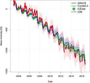
Figure 8. Comparison of cumulative mass balance trends for Arctic glaciers and ice caps for 1992–2016, based on satellite altimetry, the IOM and GRACE illustrating the agreement between the three approaches. The regions covered are 3, 4, 5, 7 and 9 in figure 1 (see also table 1).
Download figure:
Standard image High-resolution imageTable 2. Pentad mass balance rates for all land ice areas for the period 1992–2016 as plotted in figure 11. Further details about how these values were derived are provided in the supplementary data.
| Pentad | EAIS | WAIS | GrIS | GIC | TOTAL | |
|---|---|---|---|---|---|---|
| 1992–1996 | Δ mass Gt yr−1 | 28 ± 76 | −55 ± 30 | 31 ± 83 | −117 ± 44 | −113 ± 125 |
| (SLE mm yr−1) | (−0.08 ± 0.21) | (0.15 ± 0.08) | (−0.09 ± 0.23) | (0.32 ± 0.12) | (0.31 ± 0.35) | |
| 1997–2001 | Δ mass Gt yr−1 | −50 ± 76 | −53 ± 30 | −47 ± 81 | −149 ± 44 | −299 ± 123 |
| (SLE mm yr−1) | (0.14 ± 0.21) | (0.15 ± 0.08) | (0.13 ± 0.22) | (0.42 ± 0.12) | (0.83 ± 0.34) | |
| 2002–2006 | Δ mass Gt yr−1 | 52 ± 37 | −77 ± 17 | −206 ± 28 | −173 ± 33 | -405 ± 60 |
| (SLE mm yr−1) | (−0.14 ± 0.10) | (0.21 ± 0.05) | (0.57 ± 0.08) | (0.48 ± 0.09) | (1.13 ± 0.17) | |
| 2007–2011 | Δ mass Gt yr−1 | 80 ± 17 | −197 ± 11 | −320 ± 10 | −197 ± 30 | -634 ± 38 |
| (SLE mm yr−1) | (−0.22 ± 0.05) | (0.55 ± 0.03) | (0.89 ± 0.03) | (0.55 ± 0.08) | (1.76 ± 0.11) | |
| 2012–2016 | Δ mass Gt yr−1 | −19 ± 20 | −172 ± 27 | −247 ± 15 | −227 ± 31 | -665 ± 48 |
| (SLE mm yr−1) | (0.05 ± 0.06) | (0.48 ± 0.08) | (0.69 ± 0.04) | (0.63 ± 0.08) | (1.85 ± 0.13) |
For HMA, we utilise a recently published observational estimate of volume change from stereo photogrammetry covering the period 2000–2016 (Brun et al 2017). We only include those basins that are exorheic but even for these, it is likely that not all the glacial melt contributes directly to SLR (Brun et al 2017). For these basins the mean trend is −14.6 Gt yr−1 compared to a total for the whole of the High Mountains Asia of 16 Gt yr−1. This is consistent with an estimate derived from ICESat elevation changes for a shorter epoch (2003-08) (Kääb et al 2012). To extend the GIC time series back to 1992, we estimate a scaling factor from the climate-forced M15 modelled data.
In summary, where reliable observations or validated RCM simulations exist we use these and where they do not we use the original M15 global statistical modelling time series, resulting in about 86% of the mass trends being updated. Using this approach, we obtain agreement between GRACE-derived trends for 2003–2010 (Jacob et al 2012) and the statistical model simulations to within 10 Gt yr−1. Accounting for a 12 Gt yr−1 difference for HMA, we also obtain agreement with the synthesis results in Gardner et al (2013) to within 25 Gt yr−1. We partition the errors for GIC in proportion to the data source: i.e. 84% from the errors in the GRACE, RCM and stereo photogrammetry data used and 16% from the uncertainties in the statistical modelling (Marzeion et al 2017).
Figure 9 shows the results of this updated synthesis of GIC (black dashed line; excluding PGIC) compared with other published estimates. In table S6 we detail the annual rates, while the pentad values are given in table 2. There is, in general, less consistency between published studies compared to the ice sheets, with studies that use GRACE typically giving a less negative mass balance than those obtained from other methods. Marzeion et al (2017) estimated an average annual mass loss of −184 Gt from several GRACE studies for the period 2003–2009 (not including PGIC). The equivalent mass loss value from studies using other methods (WGMS 2017, Marzeion et al 2015, update from Cogley 2009); update from Leclercq et al 2011) was 230 Gt or more.

Figure 9. Post AR5 estimates of GIC mass balance and the IPCC AR5 synthesis values. Horizontal whiskers indicate the time span of the estimate. The boxes are colour-coded to reflect measurement technique used (GRACE, empirical, geodetic or direct). Vertical whiskers are the sum of quoted measurement uncertainty and the 1-sigma range due to inter-annual variability (see text for more details). Dashed line is the synthesis of observations and modelled mass balance discussed in the main text.
Download figure:
Standard image High-resolution imageThere are no studies on global GIC trends with a central year more recent than 2007, making it difficult to compare our new synthesis of GIC trends with other work over the past decade. The most recent World Glacier Monitoring Service Global Glacier Change Bulletin (WGMS 2017) suggests an average mass loss from global glaciers of ~179 Gt yr−1 and ~237 Gt yr−1 for the period 2007–2015, using direct and volume change methods, respectively (both values adjusted for PGIC by subtracting the Greenland estimate in Gardner et al 2013). These compare favourably to our estimate of 181 Gt yr−1 for the same period.
3. Synthesis
Figures 10 and 11 and table 2 summarise our synthesis of land ice mass trends discussed in section 2 (with further details provided in the supplementary data). The error bars, in this case, do not incorporate inter-annual variability and are comprised of the combined errors of the data sets used. In keeping with previous assessments, we also provide pentad means but have also plotted and tabulated the annual land ice mass balance values (figure 11 and table S6). These are useful, for example, for comparing with inter-annual estimates of ocean mass from GRACE and/or other approaches (e.g. Dieng et al 2017).
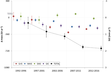
Figure 10. Pentad estimates of mass balance for the EAIS, GrIS, WAIS and GIC for the period 1992–2016 as listed in table 2. Vertical whiskers indicate the one-sigma uncertainty derived from the errors in the data used to generate the estimates. Further details about how these values were derived are provided in the supplementary data.
Download figure:
Standard image High-resolution image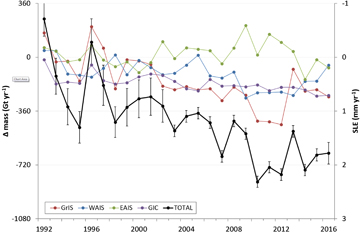
Figure 11. Our synthesis annual time series of mass trends for the ice sheets and GIC and the total SLE contribution of land ice (black line).
Download figure:
Standard image High-resolution image
Our total land ice mass contribution is smaller than some estimates from, for example, an assessment of the sum of the individual terms or GRACE-derived ocean mass (Cheng et al 2017, Dieng et al 2017) or from a global GRACE-derived land ice estimate (Jacob et al 2012). It is, however, consistent with other assessments of the total change in ocean mass (minus land hydrology) (Chen et al 2013). In the case of the GRACE-derived land ice mass trends (Jacob et al 2012), the difference, for the same period (2003–2010), is due predominantly to the difference in estimates for the AIS. Jacob et al (2012) uses the ICE-5G GIA model to correct GRACE data which over Antarctica results in a correction that is about 60 Gt yr−1 larger than more recent studies, including our synthesis, based on newer GIA solutions (Martín-Español et al 2016b). Accounting for this, results in reasonable agreement with our synthesis: −476 ± 93 and −516 ± 39 Gt yr−1, respectively. If we also substitute the most recent HMA estimate of −14 Gt yr−1, for the −4±20 Gt yr−1 used in Jacob et al this brings the numbers even closer (−486 versus −516 Gt yr−1).
Prior to the availability of GRACE data from 2003, our synthesis incorporates data from other approaches discussed previously and it is evident from figure 11 that this is reflected by larger uncertainties for the total SLE contribution. It is also interesting to note that the year-to-year differences in the total SLE can exceed 400 Gt (1.1 mm SLE). Thus, even the pentad estimates shown in figure 10 incorporate substantial inter-annual variability. This further emphasises the challenges in extrapolating a relatively short time series such as this (Wouters et al 2013b). For example, 1992 appears to be an exceptionally positive mass balance year in terms of the total land ice contribution. This coincides with maximum global cooling (of about 0.6 °C) after the eruption of Mount Pinatubo in 1991, which may be a contributory factor (Soden et al 2002).
3.1. Comparison with SLB studies
A number of studies have attempted to solve the global SLB (i.e. equation 1) by directly estimating (or synthesising published values for) all mass terms in equation (2). Others have estimated change in total ocean mass using either GRACE observations or by subtracting ∆GMSLsteric (i.e. changes in sea level due to thermal expansion and salinity, and therefore not due to mass) measured by Argo buoys from ∆GMSLTotal obtained via satellite altimetry. Table 3 shows a comparison of a selection of these studies with our synthesised land ice contributions for identical epochs.
Table 3. Published SLB estimates of ocean mass and land ice contributions derived from the sum of land ice contributions, GRACE or altimetry minus Argo (∆GMSLtotal −∆GMSLsteric ). In the case of the latter two, the inferred mass includes the land hydrology term (see equation (2)). The values in brackets indicate the difference between each estimate and our synthesis land ice contributions for identical epochs.
| Study | Time period | Δ ocean mass from sum of land ice mass contributions (mm yr−1) | Δ ocean mass from GRACE (mm yr−1) | Δ ocean mass from altimetry/Argo (mm yr−1) | Land ice sum from this study (mm yr−1) |
|---|---|---|---|---|---|
| Dieng et al 2017 | January 2004–December 2015 | 1.93 (+0.71) | 2.24 (+1.02) | 2.35 (+1.13) | 1.22 |
| Chambers et al 2017 | January 1992–December 2010 | 1.35 (+0.6) | 1.99 (+1.04) | 0.95 | |
| Chambers et al 2017 | January 2005–December 2015 | 2.11 (+0.54) | 2.20 (+0.63) | 1.67 | |
| Leuliette and Nerem 2016 | January 2005–December 2015 | 2.3 (+0.73) | 1.67 | ||
| Chen et al 2013 | January 2005–December 2011 | 1.80 (+0.24) | 1.79 (+0.23) | 1.56 | |
| Purkey et al 2014 | January 2003–December 2013 | 1.53 (0.0) | 1.53 | ||
| Purkey et al 2014 | August 1995–March 2006 | 1.47 (0.60) | 0.87 | ||
| Dieng et al 2015a | January 2003–December 2013 | 1.68 (+0.15) | 1.85 (+0.32) | 2.03 (+0.5) | 1.53 |
| Reager et al 2016 | April 2002–November 2014 | 1.58 (+0.05) | 1.53 | ||
| Rietbroek et al 2016 | January 2002–December 2014 | 1.37 (−0.16) | 1.08 (−0.45) | 1.53 | |
| Dieng et al 2015b | January 2005–December 2013 | 2.04 (+0.44) | 1.60 |
Attempting to close the SLB in this way requires consideration of the contribution of land water storage (LWS; also called terrestrial water storage, TWS). Estimates of ΔMLWS are both highly uncertain, particularly prior to the launch of GRACE, and sensitive to the epoch chosen because of the large inter-annual variability in the water cycle (Llovel et al 2011). For example, both Reager et al (2016) and Rietbroek et al (2016) estimate that LWS provides a negative contribution to the SLB (−0.33 and −0.29 mm yr−1 for the period 2002–2014, respectively), while both Chambers et al (2017) and Dieng et al (2017) attribute positive contributions (0.45 mm yr−1 for 1992–2013 and 0.25 mm yr−1 for 2004–2015, respectively). LWS adds, therefore, considerable uncertainty in attempting to close the SLB. An additional uncertainty is the influence of GIA on vertical land motion of ocean basins and the resultant change in their volume. Observations of vertical land motion in mid ocean basins are absent and rates depend on GIA models that present a substantial spread in term of the impact on absolute sea level, as measured by satellite altimetry (Tamisiea 2011).
Our estimates of SLE contributions from land ice are consistently smaller than the ocean mass estimates in the SLB studies listed in table 3 apart from one study (Rietbroek et al 2016). For example, for the epoch 1993–2015, our land ice sum produces a SLE contribution of 28 mm compared to 38 mm in Dieng et al (2017). Using our land ice estimate would not permit closure of the SLB in that study and requires a positive value for ΔMLWS and/or ΔMother. However, it is clear from table 3 that global ocean mass estimates, particularly those derived from GRACE, are currently inconsistent and present challenges for closing the SLB. An outstanding issue for these estimates is the GIA model used to correct for solid Earth effects, which have a spread equivalent to 1.4 mm yr−1 SLE but which also directly impacts the GMSL measurement made by altimetry (Tamisiea 2011). In addition, the earlier part of the satellite altimeter record of GMSL (relevant to column five in table 3), obtained from Topex/Poseidon is subject to a drift term that has been accounted for in some studies but not others (Watson et al 2015). There are also small, but non-random, effects from other factors including ocean floor deformation (Frederikse et al 2017) and water vapour (e.g. Dieng et al 2017).
4. Summary and outlook
In this review, we have concentrated, primarily, on post-AR5 estimates of the land ice contribution to SLR from 1992–2016, and compiled a single time series of global ice mass trends for this period (figure 11).
Since 2003, in particular, with the addition of GRACE data, uncertainties in both ice sheet and GIC contributions have been reduced and agreement between GIC estimates has improved significantly (Marzeion et al 2017). Despite some issues of signal to noise limitations for smaller GIC sectors, and acknowledging the uncertainties associated with High Mountains Asia, we have demonstrated that GRACE can provide unbiased land ice trends. Incorporating other techniques such as satellite-based stereo photogrammetry (e.g. Brun et al 2017) and altimetry for regions with poor signal to noise (Scandinavia, Central Europe, Caucasus, low latitudes and New Zealand) has reduced the trend uncertainties and provides an optimised global approach.
Taking this approach, our combined land ice contribution for the satellite era is in broad agreement, for example, with the AR5 synthesis for the ice sheets up to 2012, (figures 5, 6 and 7) and at the lower end for GIC up to 2010 (figure 9). For the most recent 5 year period (2012–2016 in table 2), we found an average global contribution of 665 Gt yr−1 (1.85 mm yr−1 SLE), with Greenland contributing 37% (247 Gt yr−1 or 0.69 mm yr−1 SLE) and GIC contributing 34% (227 Gt yr−1 or 0.63 mm yr−1 SLE). Antarctica as a whole contributed the remainder, though the vast majority was from WAIS (172 Gt yr−1 or 0.48 mm yr−1 SLE) with EAIS close to balance.
Our land ice contribution time series results, in general, in a smaller contribution to SLR than other assessments of both individual components of ∆GMSLmass and SLB estimates based on the total change in mass of the ocean (e.g. Chambers et al 2017, Dieng et al 2017). There are several possible reasons for this. First, the largest difference is in our GIC estimates where we use an updated statistical modelling time series (Marzeion et al 2017) that has lower mass loss rates compared to the previous version. In addition, for several regions, we have substituted modelled values for 2003–2016 with observation-based estimates (from GRACE and, for HMA, from satellite stereo-photogrammetry), all of which have lower mass loss values. This means we obtain a mean mass contribution of 189 Gt yr−1 (0.53 mm yr−1 SLE) for 2003–09 compared with, for example, 215 Gt yr−1 in the consensus study of Gardner et al (2013). Most of the difference between these values is explained by our lower estimate for the HMA (14.5 vs 26 Gt yr−1).
Second, for the GrIS, we use a new 1 km downscaled version of the regional climate model that results in a marginally smaller mass loss for the period 1992–2002 compared with previous IOM trends (e.g. Van den Broeke et al 2016) of about 0.1 mm yr−1 SLE. Third, the most recent GIA solutions for Antarctica are converging on a smaller mass correction for GRACE data compared with earlier solutions (Martín-Español et al 2016b). The difference is as much as 60 Gt yr−1 or the equivalent to 0.2 mm yr−1 SLE when using GRACE data to determine AIS trends. Finally, we have taken care to ensure that PGIC are not double counted in our time series. This has occurred in some, but not all, previous studies and, in particular, in SLB assessments where the authors may be unaware that the ice sheet mass trends implicitly include PGIC, but where they are also included in the GIC trends used (e.g. Dieng et al 2017). In Greenland, the PGIC contribution is on the order of 0.1 mm yr−1 (table 1). These three factors, combined, could be responsible for as much as a 0.4 mm yr−1 difference for the land ice contribution to SLR. Combined, our updates and improvements to previous land ice time series have resulted in a reduction of 6±1.1 mm SLE compared to a recent SLB estimate of the land ice contribution for 2003–2015 (Dieng et al 2017), equivalent to a difference of 0.46 mm yr−1. Our smaller land ice contribution makes closing the SLB, potentially, more challenging. It implies a positive contribution from land hydrology and/or other factors such as a GIA trend on ocean basin volume closer to the lower end of estimates of −0.15 mm yr−1 (Tamisiea 2011).
Whilst it has been instructive to compare our land ice time series with SLB estimates of ocean mass (table 3), either from GRACE or from altimetry minus Argo (∆GMSLtotal −∆GMSLsteric), uncertainties in global GIA (e.g. Tamisiea 2011, Spada 2017), low degree and order corrections to GRACE, steric estimates for high latitudes and the deep ocean and the land hydrology component of the SLB limit the value of a quantitative comparison with our land ice time series. We note, in addition, that there is a large spread in GRACE-derived ocean mass trends in table 3, varying by more than a factor of 2, which cannot be explained by the slightly different epochs used. Nonetheless, with a longer time series of observations, improvements in the corrections mentioned above and the addition of GRACE follow on data, SLB assessments will be a helpful tool for constraining land ice mass trends.
The GRACE mission ended in September 2017 with the failure of one of the satellites and the quality of the data during the last year of the mission was degraded due to aging electronics. A GRACE follow on mission was launched in May 2018 and, with a successful deployment, will provide continuity of gravity-derived mass trends over land ice. CryoSat-2 is still in orbit and has enough fuel to last until at least 2020, continuing the elevation change measurements over the ice sheets and larger ice caps that began in 2010. In addition, the next generation laser altimeter mission, ICESat-2, also has a planned launch date of 2018. With three pairs of beams, this system will provide improved coverage of GIC, in particular, offering an additional measurement tool for land ice trends (Markus et al 2017). Together these satellite missions will provide unprecedented accuracy and resolution over land ice globally and help further refine and improve our understanding of land ice contributions to contemporary sea level rise. They will also provide robust and reliable calibration and validation for statistical scaling and numerical modelling approaches that can, and have been, used to extend the mass trend record back in time (e.g. Leclercq et al 2011, Marzeion et al 2015) and for projecting future changes, driven by climate forcing scenarios. We have developed, and presented, a well constrained and robust record of the land ice contribution to SLR for the last 25 years. With successful deployment of slated satellite missions, we have the potential for both improved accuracy and resolution for monitoring land ice trends in the future.
Acknowledgments
JLB and RMW were supported by the European Research Council (ERC) under the European Union's Horizon 2020 research and innovation programme under grant agreement No 694188 (GlobalMass). JLB was also supported by a Leverhulme Trust Fellowship RF-2016-718. The authors would like to thank the following colleagues for providing datasets used in this study: Valentina Barletta; Stephen Chuter; Ellyn Enderlin; Andreas Groh; Martin Horwath; Bryant Loomis; Scott Luthcke; Ingo Sasgen; Ernst Schrama; Michiel van den Broeke; and David Wiese.