

Abstract
Georeferenced information on road infrastructure is essential for spatial planning, socio-economic assessments and environmental impact analyses. Yet current global road maps are typically outdated or characterized by spatial bias in coverage. In the Global Roads Inventory Project we gathered, harmonized and integrated nearly 60 geospatial datasets on road infrastructure into a global roads dataset. The resulting dataset covers 222 countries and includes over 21 million km of roads, which is two to three times the total length in the currently best available country-based global roads datasets. We then related total road length per country to country area, population density, GDP and OECD membership, resulting in a regression model with adjusted R2 of 0.90, and found that that the highest road densities are associated with densely populated and wealthier countries. Applying our regression model to future population densities and GDP estimates from the Shared Socioeconomic Pathway (SSP) scenarios, we obtained a tentative estimate of 3.0–4.7 million km additional road length for the year 2050. Large increases in road length were projected for developing nations in some of the world's last remaining wilderness areas, such as the Amazon, the Congo basin and New Guinea. This highlights the need for accurate spatial road datasets to underpin strategic spatial planning in order to reduce the impacts of roads in remaining pristine ecosystems.
Export citation and abstract BibTeX RIS

Original content from this work may be used under the terms of the Creative Commons Attribution 3.0 licence.
Any further distribution of this work must maintain attribution to the author(s) and the title of the work, journal citation and DOI.
Introduction
Roads are important for socio-economic development by providing access to resources, jobs and markets [1–5], but they also bring about various direct and indirect environmental impacts. For example, road construction and use lead to increased emissions of greenhouse gasses and air pollutants, including carbon dioxide, nitrogen oxides and fine particulate matter, which in turn lead to climate change as well as adverse health effects [6–8]. Ecosystems and wildlife are affected mainly because roads provide access to otherwise undisturbed areas. This results in habitat fragmentation, deforestation, and reduced wildlife abundance though disturbance, mortality (road kills) and overhunting, particularly in tropical regions [9–13]. Further, roads may exacerbate societal inequities. For example, only farmers with sufficiently high output might be able to afford and benefit from bulk transportation services, which gives them a competitive advantage over smaller farmers [14].
To adequately quantify the benefits as well as the impacts of roads, accurate and up-to-date georeferenced information on the global road network is essential [15]. Possible applications of such data include global-scale estimations of travel time and accessibility, quantification of road transport and associated emissions, biodiversity impact assessments, and explorations of options to reduce impacts [5, 8, 11, 15, 16]. Global road data is typically retrieved from the Vector Map Level 0 (VMAP0) dataset from the United States National Imagery and Mapping Agency [17]. VMAP0 (covering the period 1979–1997) comprises approximately 7.4 million km of road, which is only a minor share of the total road length as reported in national statistics [15, 18]. The gRoads initiative [19] substantially increased the road coverage for specific countries, but it still remains largely based on VMAP0 data. This also applies to commercial products, such as the ADC worldmap and Global Discovery dataset [20, 21]. Commercial high-resolution datasets intended for navigation have also been produced [22, 23], but these are not freely available. Moreover, the spatial coverage of these commercial datasets is biased towards Europe, North America and large urban areas. This limitation also holds for the crowdsourced information available from the OpenStreetMap project [24, 25], due to the opportunistic approach to data collection. This means that current public-domain global road maps are either outdated or that their coverage is strongly geographically biased.
Over the last decade, digital georeferenced data on roads are becoming increasingly available online, and the manifestation of numerous thematic and national spatial data infrastructures (SDIs) facilitates the discovery of these road network datasets [26, 27]. Driven by the need to improve the coverage of georeferenced global road data as well as the increasing availability of road data in the public domain, we initiated the Global Roads Inventory Project (GRIP). The primary aim of GRIP was to gather and integrate existing publicly available georeferenced roads datasets into a consistent global roads dataset. In addition, we aimed to explore and quantify possible relationships between road construction and ultimate socio-economic drivers, which may serve to obtain estimates of future infrastructural expansion.
To create the GRIP dataset, we selected, combined and harmonized publicly available national and supra-national vector datasets from governments, research institutes, NGOs and crowdsource initiatives into one global dataset. Apart from the vector dataset, we also compiled gridded layers for road length (km of road per cell) and road density (meters of road per km2 land area per cell) on a 5 × 5 arcminute resolution (approximately 8 × 8 km at the equator). In order to quantify possible relationships between road construction and socio-economic drivers, we then performed a multiple linear regression analysis where we related the total road length per country, as retrieved from the GRIP dataset, to four explanatory variables: the countries' total land surface area, human population density, gross domestic product per capita (GDP; in international PPP US$) and OECD membership (yes or no) [28, 29]. Thus, we cover both human population and affluence, which are generally considered two main ultimate drivers of environmental impact [30]. Finally, we applied our regression models to obtain country-level estimates of the total additional road length for the year 2050, based on projections of GDP and population density according to the so-called Shared Socioeconomic Pathway (SSP) scenarios [31], i.e. a coherent set of scenarios describing five alternative socio-economic futures.
Data and methods
Data gathering and selection
To compile the GRIP dataset we combined the best available (supra-)national geospatial road data. We searched for data from organizations and activities that are responsible for or have an interest in spatial data on road infrastructure. This included United Nations (UN) organizations like the Logistics Cluster of the World Food Programme, the Food and Agriculture Organization, the Organization for the Coordination of Humanitarian Affairs and the High Commission on Refugees. We also searched for data via international research organizations and non-governmental organizations (NGOs). Crowdsourced data initiatives were searched for to cover gaps in the (supra-)national datasets.
For the (supra-)national datasets, the following selection criteria were defined for inclusion in GRIP:
- The selected dataset has a supra-national or national coverage, in order to prevent the sub-national bias in network coverage that characterizes existing global roads datasets due to fragmented digitization of map tiles, varying intensity of crowdsourcing activities and the occasional inclusion of detailed sub-national fragments of data [5, 15, 32]. If more than one data source was identified for a country, they were compared and combined to achieve the best national road network coverage.
- The error in the spatial positional accuracy is maximum 500 meters, as derived from meta-data or determined based on visual comparison with the VMAP data, digital and paper atlases, official topographic maps and remote sensing images from Google Maps, ESRI Basemaps and other available sources, using ArcGIS.
- The attribute information should include an indication of road type, in order to facilitate classification into one of five commonly applied functional road types [19, 33, 34]: highways, primary roads, secondary roads, tertiary roads and local roads.
- The scale should range between 1:100 000 and 1:500 000, in order to reduce spatial bias in road coverage induced by large differences in scale.
- The temporal coverage of the dataset should be as recent as possible and at least exceed the VMAP0 dataset (>1997).
- The dataset is publicly available in order to ensure that the GRIP database can be easily shared with others.
Crowdsourced OpenStreetMap data were used to cover Europe, as best available seamless dataset, and China, because of a lack of publicly available data from government or research institutes. OpenStreetMap data were further used for 200 cities worldwide with a population of more than 1 million people. In total 35% of the global road length in GRIP is derived from OpenStreetMap. An overview of all data sources used in GRIP is provided in tables S1 and S2 available at stacks.iop.org/ERL/13/064006/mmedia.
Data model for harmonization
To harmonize the road attribute information among the different source datasets, we applied the UNSDI-Transportation data model. The UNSDI-Transportation data model is a globally applicable transportation network attribute description designed by the United Nations Logistics Cluster [34]. It defines and categorizes various relevant attributes of roads, such as road type, pavement type and seasonality. Its description of road characteristics is commonly used in UN operations globally and other data initiatives that harmonize transportation information across countries [19, 33, 35, 36]. Following this data model, we classified each road segment into one of five distinguished functional road type categories: highways, primary roads, secondary roads, tertiary roads and local roads. We included surface pavement attributes because paved highways typically have much larger environmental impacts than unpaved roads, especially in wet environments where unpaved roads can become seasonally impassable [37], which in turn could also affect humanitarian operations. In case information on seasonality was lacking, unpaved rural secondary/tertiary roads in tropical regions were classified as having seasonal availability.
Data handling and integration
All datasets were re-projected to the WGS84 geographic coordinate system. If the original projection information of the dataset was unknown, the details were derived from the source, national mapping agencies or manually defined. To achieve coverage of all defined road types, for some countries multiple data sources were combined to create the best representation of the national road network (see table S2 for data sources used per road type per country). Then, in order to clean the dataset and reduce the number of line segments to optimize performance for analyses, a single features 'dissolve' operation on the road type attribute was performed. Next all remaining attributes were added and classified based on the available source information. Finally, a global coverage dataset was created by first merging country datasets into continental datasets and subsequently merging those into one global dataset. Highway and primary road network connections across country borders were visually inspected and discontinuities were repaired if needed. We did this by manually reconnecting the line elements for discontinuities larger than 50 m and using the 'extend line' tool in ArcGIS to repair smaller discontinuities, whereby we verified the locations of the road using ESRI satellite imagery basemaps in ArcGIS. All data handling and integration was performed in ArcGIS, with version 9.1 through 10.3.1 [38].
Raster datasets
In addition to the vector dataset, we produced global road density raster layers (road length per unit of area) at a resolution of 5 arcminutes (approximately 8 × 8 km at the equator). To that end we overlaid the road vector dataset with a global 5 arcminute 'fishnet' vector dataset with unique cell identifiers and assigned all road vector elements within a given cell the corresponding cell ID. We then calculated the length (in meters) of each individual road vector element in ArcGIS, accounting for the distance distortion in the WGS84 coordinate system, and summed the lengths per cell ID for each of the individual road types. The resulting table was joined to the fishnet vector dataset, which was then converted to 5 arcminute raster datasets using the summed road length per road type. Finally, the 5 arcminute road length rasters were divided by a matching 5 arcminute resolution area (km2 per cell) raster [39] to derive road densities (in m per km2).

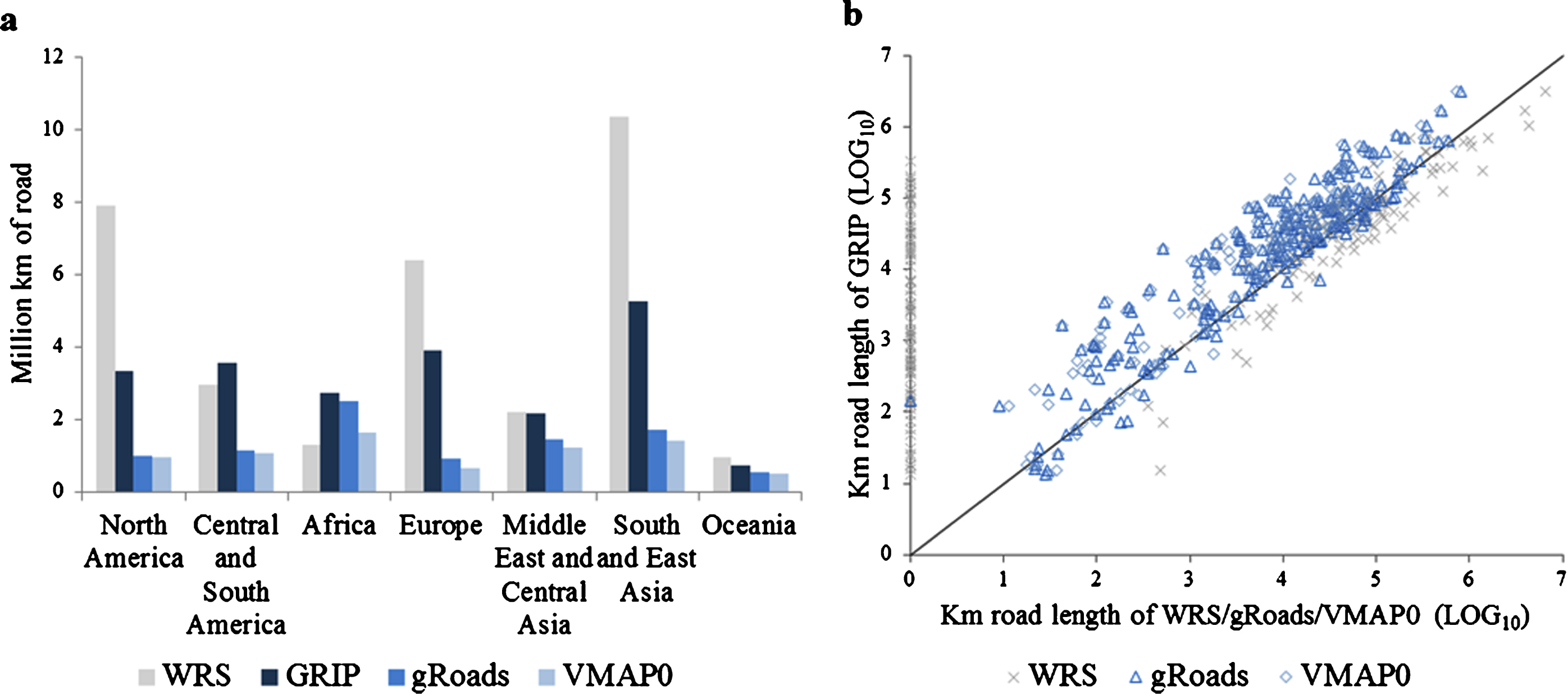
Figure 1. Road network length included in GRIP as compared to the geo-referenced global road datasets VMAP0 and gRoads and the country-level non-spatial data in the World Road Statistics (WRS) database, (a) per region and (b) per country. The comparison per country is based on the log10-transformed total road length (km) with +1 added prior to the log-transformation. WRS data represent 10 year averages over 2005–2014.
Download figure:
Standard image High-resolution imageRegression analysis
After establishing the dataset, we performed a multiple linear regression analysis where we related road length to four explanatory variables: area, human population density, gross domestic product (GDP) per capita and OECD membership. We did this analysis on a country level, because this matched best with both the scope of the road data collection in GRIP and the availability of current and future explanatory variable data. We retrieved country-specific data on land surface area (km2), population size (n) and GDP per capita (purchasing power parity (PPP) corrected, in current international US$) from the World Bank and obtained population density by dividing the population size by the land surface area. For countries not included in the World Bank database, we retrieved data from additional sources (mainly the CIA World Fact Book or Wikipedia; see table S3). For both population size and GDP per capita, we used values from the most recent year with data available (mostly 2015; table S3). We then took the countries with data available for all response and explanatory variables (n = 219) and log10-transformed all continuous variables because of the skewed data distribution (table S4). As zero values cannot be log-transformed, we added +1 to all road length values prior to the transformation. Variance inflation factors (VIFs) of the four explanatory variables were well below 2 (country area = 1.62, human population density = 1.40, GDP = 1.37, and OECD = 1.33), indicating limited multicollinearity [40, 41]. To account for possible levelling off of the effects of affluence or population density on road length, we added the squared terms of these explanatory variables to our regression models. To prevent overfitting, we performed a step-wise variable selection procedure to identify the most parsimonious model, using the Bayesian Information Criterion (BIC) as selection criterion, and allowing a quadratic term only if the corresponding linear term was also included. We evaluated the resulting regression models based on Cook's distance values and residual plots. Cook's distances were all well below 1, indicating that none of the observations had an undue influence on the regression coefficients [42]. The residuals were randomly distributed and outliers (absolute standardized residuals > 3) were restricted to cases where zero road length was observed (figure S3). Finally, to test the predictive ability of our models, we performed a three-fold cross-validation, using 146 countries for model training and 73 for testing, such that each country was within the test set once. All statistical analyses were performed in the R environment [43].
Projecting future road length
For the future projections we used the regression model for total road length only. This model performed equally well on the training and independent test data (cross-validated mean R2 of 90%), whereas the cross-validation results showed considerably lower and more variable performance of the regression models for specific road types (table S5). We applied our regression model to obtain estimates of the total additional road length for the year 2050, based on projections of GDP and population density according to the so-called shared socio-economic pathway (SSP) scenarios, i.e. a coherent set of scenarios describing five alternative socio-economic futures. The SSPs are based on five narratives describing alternative socio-economic developments, including sustainable development, regional rivalry, inequality, fossil-fueled development, and middle-of-the-road development. The three main socio-economic drivers of the scenarios are population, urbanization and gross domestic product [31]. For our projections of future road length, we retrieved country-specific projections of population growth and GDP from the IIASA SSP portal [44]. Data were available for 165 of the 222 countries included in GRIP (representing 97% of the present-day total road length). In the projections we assumed that the road network in a given country would not shrink, i.e. if future population size and per-capita GDP resulted in projected road lengths smaller than the present-day estimate, the present-day estimate was retained (as presented in table S6).
Results
Coverage of the global road network
The GRIP dataset comprises more than 21.6 million km of roads in total. This is a considerable improvement over the VMAP0 and the gRoads datasets, which cover 7.4 and 9.1 million km, respectively (figure 1). Yet, the total global road length in GRIP is mostly smaller than suggested by the World Road Statistics (WRS) database, which contains non-spatial country-level road length estimates [18]. Over 50% of the road length included in GRIP is from data sources published in 2010 or later. A further 23% is from data sources published between 2006 and 2010 and 14% was published between 2000 and 2005. Only 8% is still based on the VMAP0 data (table S1). Improved coverage compared to the earlier geo-referenced datasets was especially apparent for North America, South and Central America, Europe, and South and East Asia (figure 1(a)). For regions were GRIP relies mainly on VMAP0 data, such as the Russian Federation and several other Central Asian countries, only a slight increase in road length coverage was obtained.

Figure 2. (a) Distribution of road length over the different road types in the GRIP dataset compared to VMAP0 and gRoads, and (b) road length plotted against rank on a log10 transformed scale, with road types ranked starting from highways (type 1).
Download figure:
Standard image High-resolution imageThe more recent gRoads initiative (2013) mainly focused on finding data sources that helped improve coverage in Africa [19]. These data sources were also included in GRIP, which explains the relatively small difference in total road length between the two global datasets for this region. Yet, for 186 countries worldwide, GRIP covers a larger part of the road network compared to VMAP0 and gRoads (figure 1(b)). In a few cases the total road length in GRIP was (slightly) lower compared to VMAP0 or gRoads. These included small (island) states like Bermuda, Cook Islands, Niue, Palau and Wallis and Futuna, which have very small road networks, hence an uncertainty of just a few kilometers may result in a relatively large deviation between the different datasets (figure 1(b)).
Road type distribution
On a global scale, the distribution of the total length of the road types 1, 2, 3 and 4 (figure 2(a)) resembles a pattern that is commonly found when roads are hierarchically classified into roads that enable fast long-distance mobility as opposed to roads that increase local accessibility. This typically results in relatively few kilometers of highways and primary roads and a larger length for secondary and tertiary roads [45, 46]. In the VMAP0 and gRoads datasets, a similar pattern was observed for road types 1–3, but not for type 4 (figure 2(a)).
In the GRIP data, the distribution of the total length across the first four road types appeared to follow a power law, with the total length per road type nearly doubling with each increase in rank from the highways (rank 1) to the tertiary roads (rank 4) (figure 2(b)). Power law distributions between frequency of occurrence or size on the one hand and rank on the other are commonly observed in a wide variety of phenomena, including the frequency of words in texts, population sizes of cities, and size distributions of earthquakes, although the power law does not always hold over the entire range [47, 48]. The total length of the local roads (type 5) clearly deviated from the power-law distribution. This suggests that local roads in particular may be underrepresented in the GRIP dataset, likely due to geographical bias in data availability. Many of the country-level datasets incorporated in GRIP have only limited coverage of local roads. The majority of the local roads in GRIP (almost 60% of the total length) have been derived from OpenStreetMap, thus including its bias in coverage towards more developed regions and large urban areas [25].
Global patterns in road density and quality
The global GRIP road maps show clear spatial variability in road density (figures 3 and 4). In general, the highest road densities were observed in Northwest Europe and parts of South and East Asia. Roads are rare or even absent in the northern parts of Canada and the Russian Federation, the Sahara desert and large parts of the Amazon forest. The maps confirm a spatial bias in coverage for the local roads (type 5; figure 3). For various countries in South America, Africa and Asia, the coverage of local roads is less dense compared to other regions and other road types, and mainly limited to larger urban areas (see also table S3). Road surface type and accessibility information was available for 75% of the total road length covered in GRIP (see figure S1). Globally we found that 35% of the roads are paved and 50% of the roads have all year accessibility. Most paved roads are found in North America and Europe, whereas most unpaved and only seasonally accessible roads are found in Central and South America and Africa.

Figure 3. The GRIP global road maps, displaying the detailed and harmonized coverage over world regions and the coverage per individual road type.
Download figure:
Standard image High-resolution image
Figure 4. GRIP global road density map on 5 arcminute resolution (approximately 8 × 8 km at the equator), representing the densities summed across the five road types.
Download figure:
Standard image High-resolution image
Figure 5. Total road length per country (n = 222) as obtained with multiple linear regression models (table 1) compared to the values observed for (a) all roads combined and (b) per sub-type. Values represent log10-transformed total road length (km) with +1 added prior to the log-transformation. Main roads include highways and primary roads.
Download figure:
Standard image High-resolution image
According to our road length regression models, total road length in a country is strongly and positively related to its total land surface area, human population density, gross domestic product and OECD membership (table 1; figure 5). The variation explained by the regression models ranged from 63% for the local roads to 90% for all road types combined (figure 5), which is larger than existing country-level regression models [28, 29, 49]. The positive relationships of road length with GDP, OECD membership and population density reflects that road densities are higher in developed countries with higher GDP, like those in Northwest Europe, as well as more densely populated countries like India, Bangladesh and Rwanda (figure 3; figure 4).
Table 1. Regression coefficients (with standard error) of multiple linear regression models relating the total road length in a country to country area (km2), population density (n km−2 in 2015), GDP per capita (international $, PPP, in 2015) and current OECD membershipb. All continuous variables were log10-transformed. NA indicates that the explanatory variable of concern was not included in the most parsimonious regression model.
| Explanatory variables | Regression coefficients | ||||
|---|---|---|---|---|---|
| All roads | Main roadsa | Secondary roads | Tertiary roads | Local roads | |
| Intercept | −1.66 (0.29) | −5.23 (0.52) | −3.18 (0.53) | −3.46 (0.40) | −7.83 (0.85) |
| Area | 0.90 (0.02) | 1.01 (0.04) | 0.92 (0.04) | 1.15 (0.05) | 1.07 (0.07) |
| population density | 0.52 (0.04) | 0.80 (0.08) | 0.47 (0.09) | 0.84 (0.11) | 1.26 (0.12) |
| GDP | 0.13 (0.05) | 0.51 (0.09) | 0.31 (0.09) | NA | 0.75 (0.15) |
| OECD membership | 0.36 (0.07) | 0.36 (0.13) | NA | NA | 0.97 (0.21) |
aMain roads include highways and primary roads. bSee table S3 for per-country data specification.
Road length scaled with land surface area with a coefficient close to 1, while generally smaller regression coefficients were found for the socio-economic variables. This may reflect that increases in population density and GDP result not only in the construction of new roads, but also an increased use of existing roads [28, 50]. For local road length, however, relatively large regression coefficients were observed for population density, GDP and OECD membership (table 1). This might reflect bias in the availability of crowdsourced data on local roads towards more densely populated and prosperous regions.
Projecting future road length
SSP projections for GDP and population density were available for 165 of the 222 countries included in GRIP, together accounting for 97% of both the total land surface area and total road length of the countries in GRIP. The total additional road length projected for 2050 ranged from 3.0 million km for SSP scenario 4 to 4.7 million km for SSP scenario 5 (table 2). These differences were driven mainly by differences in economic growth, as SSP4 combines moderate global population growth with relatively low increases in per-capita GDP, whereas SSP5 combines relatively low population growth with very rapid economic development that converges among countries [31]. When averaged over the five SSP scenarios, most additional road kilometers are expected in Africa, South and East Asia and South America (figure S2). On a country level, the largest absolute increases in road length were observed for the USA, India, Australia, Canada and China (table S6). Considerable increases were also found for developing nations in some of the world's last remaining wilderness areas, such as the Democratic republic of Congo (+81%), Nigeria (+52%), Papua New Guinea (+50%) and Brazil (+10%). This reflects that these countries are projected to undergo relatively large increases in population density and/or GDP according to the SSP scenarios.
Table 2. Global road length estimates (in million km and percent change) for 2050 for each of the five SSP scenarios, obtained by applying the road length regression models (table 1) to country-specific projections of GDP and population size as available for 165 countries. Country-specific road length estimates are provided in table S6.
| Scenario | Total road length (106 km) | Change (%) |
|---|---|---|
| Present daya | 20.2 | — |
| SSP1: Sustainable development | 23.8 | 18% |
| SSP2: Middle-of-the-road | 24.0 | 19% |
| SSP3: Regional rivalry | 23.3 | 15% |
| SSP4: Inequality | 23.1 | 14% |
| SSP5: Fossil-fueled development | 24.8 | 23% |
aFor comparability, present-day totals were calculated over the same 165 countries for which future projections could be made.
Discussion
The Global Road Inventory Project has resulted in a globally harmonized road network database covering a larger part of the road network than the currently available country-based global road datasets VMAP0 and gRoads. Differences in road patterns between GRIP and the earlier global road datasets reflect not only the construction of new roads, but also an increase in data coverage (i.e. GRIP filling gaps in earlier maps). Moreover, information on the year of construction was not available in the data sources used to construct GRIP. Hence, the datasets cannot be directly used in order to quantify historic road expansion. The total road length in GRIP (21.6 million km) is smaller than suggested by the World Road Statistics (WRS) database [18], which reports a global total of 32 million km of roads as the sum of country data averaged over the period 2005–2014. It should be noted that the WRS dataset is characterized by considerable differences in road length estimates and road type definitions per country over the years reported. Also between countries the methodologies for measuring road length differ, for example, according to the limited WRS metadata, some countries include dual carriageways, sidewalks, non-public farm roads or measure road length by traffic directions. Without further detail, this implies that the reliability of the WRS information and the usability for comparison is limited. Yet, the difference in total road length between GRIP and WRS indicates that the coverage of GRIP can be further improved (figure 1). On a global scale, 68% of the road network length averaged over 2005–2014 reported by WRS is classified as type 'other roads'. In GRIP the corresponding local roads class constitutes 23% of the total road network. This confirms our finding that future improvements in GRIP should focus in particular on the representation of the local roads (figure 2). Moreover, given that a large proportion (34%) of the GRIP data originates from official governmental sources (table S1), unofficial roads are currently likely underrepresented. Unofficial or unplanned roads may make up an increasing share of the road network particularly in relatively pristine areas, such as the Amazon and the Congo basins, driven by the private sector that constructs roads without government permission in order to exploit natural resources [37, 51, 52].
Until recently, geospatial information was typically compiled by national mapping agencies or private sector firms with sufficient financial and technological resources available. Over the past decade, additional road data collection methods and sources have become available, including (semi)-automated extraction from remote sensing imagery, GPS tracking, and crowdsourcing [53, 54]. In GPS tracking, large quantities of GPS tracks, for example from recreational traveling, are merged to produce mapped road segments. Currently, both GPS tracking and (semi-)automated extraction of road data from remote sensing imagery are still in the experimental phase, with approaches being developed to clean the data from positional inaccuracies and false or missing road segments [53, 54]. Hence, these methods could not yet be routinely applied at the global scale during the construction of the GRIP dataset, but they might come in useful for future improvements of GRIP, particularly to fill the gaps for unofficial roads in pristine areas [51]. Crowdsourcing is a workflow to gather data that might be collected through multiple methods. OpenStreetMap (OSM) is a well-known crowdsourced collaborative project and considered a prominent example of volunteered geographic information collection. OSM constituted an important data source for GRIP in the European Union, where its high precision and wide coverage make it the best available seamless dataset [25, 55–57]. Beside technical issues of importing OSM datasets in ArcGIS, the main challenges for using national-coverage OSM data in GRIP were identified as the validation of the data coverage, the use of multiple parallel line elements to represent segregated roads (e.g. motorways and highways), and the clear differences in coverage between urban and rural areas [32]. All these issues can largely be attributed to the volunteered and piecemeal data gathering approach of OSM [5, 11, 32], which currently results in a high coverage in densely populated developed regions (notably urban areas in Europe and North America) but varying in developing regions.
Various factors may promote road expansion, including pursuits for natural resources (timber, ores) and further agricultural development [37, 58] as well as policies to stimulate economic development [1, 4, 59]. In our regression models we accounted for two ultimate drivers of road development only (population and affluence), which are not necessarily representative of all relevant proximate factors underlying road expansion. Moreover, in absence of reliable time series data, we had to use a cross-sectional rather than longitudinal regression modelling approach ('space-for-time' substitution). Given the limitations of the regression model, our projections should be considered as first-tier estimates of future road expansion at the country level. Future research may focus on more spatially explicit modelling of future road network changes. According to our tentative projections, road length will increase by 3.0 to 4.7 million km in 2050, which represents an increase of 14%–23% compared to the present-day estimate (table 2). In comparison, Dulac [60] estimated future road length based on projected future vehicle travel (km) and arrived at an estimate of 14.8–25.3 additional million km of paved-lane road length by 2050, which represents an increase of about 35%–60% compared to the approximately 43 million km of paved lane length as estimated for 2010. Although the estimates are difficult to compare due to differences in methodology and underlying data, this suggests that our estimates, focusing on roads instead of paved lanes, are relatively conservative.
Against the expected future increase in roads, the effectiveness of land use planning is seen as a crucial element in successfully dealing with various tradeoffs involved in road construction [37, 58]. This is even more so given that the largest increases in road length are foreseen for developing nations in some of the world's last remaining wilderness areas, such as the Amazon, Congo basin and New Guinea (table S6). To inform and support global policy analysis and spatial modelling of future road developments and their related impacts, up-to-date and accurate data on roads are needed. With GRIP, we have provided a major step towards a more representative, consistent and harmonized global road map.
Acknowledgments
We would like to thank Kees Klein Goldewijk for his long term encouragement to create GRIP, the UN Logistics Cluster for assisting us in the use of the UNSDI-T data model, Eddy Scheper, Anke Keuren and Eiso Zanstra for their help with data collection, harmonization and integration, Alex de Sherbinin for organizing interest in this challenge via the CODATA Global Roads Task Group, the OpenStreetMap foundation for access to their data and Ana Benítez López and Lex Bouwman for proof-reading the manuscript. We also thank five anonymous reviewers for their valuable and constructive comments, which greatly helped us to improve the manuscript.
The GRIP dataset (vector data and 5 arcminute raster layers) can be downloaded from www.globio.info/download-grip-dataset