

Abstract
Historical changes in soil carbon associated with land-use change (LUC) result mainly from the changes in the quantity of litter inputs to the soil and the turnover of carbon in soils. We use a factor separation technique to assess how the input-driven and turnover-driven controls, as well as their synergies, have contributed to historical changes in soil carbon associated with LUC. We apply this approach to equilibrium simulations of present-day and pre-industrial land use performed using the dynamic global vegetation model JSBACH. Our results show that both the input-driven and turnover-driven changes generally contribute to a gain in soil carbon in afforested regions and a loss in deforested regions. However, in regions where grasslands have been converted to croplands, we find an input-driven loss that is partly offset by a turnover-driven gain, which stems from a decrease in the fire-related carbon losses. Omitting land management through crop and wood harvest substantially reduces the global losses through the input-driven changes. Our study thus suggests that the dominating control of soil carbon losses is via the input-driven changes, which are more directly accessible to human management than the turnover-driven ones.
Export citation and abstract BibTeX RIS

Original content from this work may be used under the terms of the Creative Commons Attribution 3.0 licence.
Any further distribution of this work must maintain attribution to the author(s) and the title of the work, journal citation and DOI.
1. Introduction
Land-use change (LUC), for example, the transformation of natural vegetation to crops or pastures and the related land management practices, contributes substantially to changes in soil carbon. Analysis of local-scale measurements, which monitor the response of soil carbon to different LUCs, indicate that the magnitude and direction of the changes differ depending on the type of LUC (e.g. Don et al 2011, Poeplau et al 2011). Bookkeeping models and dynamic global vegetation models (DGVMs) that are used to quantify LUC effects on the terrestrial carbon estimate a global soil carbon loss ranging from 0 to 100 Pg C over the 20th century (e.g. Houghton 2003, Tian et al 2015). The dominant effect of soil carbon losses by deforestation is counteracted to a smaller extent by recent reforestation efforts, which have led to soil carbon gain for some regions in the late 20th century (e.g. Houghton et al 1999, Liski et al 2002). Despite the awareness that past LUCs have resulted in a global loss of soil carbon, a key question remains unanswered: how do the different controls that influence changes in soil carbon following LUC contribute to the total change?
Changes in soil carbon are generally controlled by changes in the quantity of litter inputs from the vegetation to the soils (input-driven) and turnover of carbon in the soil, which is highly dependent on the quality of litter (turnover-driven). For example, replacing natural vegetation dominated by woody vegetation types with pastures or croplands often leads to less biomass in the vegetation, which decreases the litter input. Furthermore, woody litter decomposes more slowly than non-woody litter; hence the turnover of litter and soil carbon is generally slower in forests compared to pastures or croplands. In addition to vegetation productivity and soil decomposition, there are processes that influence the litter fluxes to the soil and the carbon losses from the soil to the atmosphere. Natural disturbances via windthrow contribute to the transfer of vegetation biomass to the soils. In addition, vegetation fires, that occur naturally or are induced by humans, lead to carbon losses from both the vegetation and soil to the atmosphere. Previous studies have shown that the additional litter input associated with windthrow increases soil carbon (e.g. dos Santos et al 2016), whereas forest fires tend to decrease soil carbon via losses in the litter carbon to the atmosphere (e.g. Liski et al 1998). Therefore, these processes also contribute to the input-driven and turnover-driven changes in soil carbon.
Historical soil carbon losses not only result from anthropogenic changes in land cover, but also from land management: 42%–58% of the ice-free land surface is managed to satisfy human needs without changing the type of land cover (e.g. forestry) (Luyssaert et al 2014). About 8.18 Pg C yr−1, which represents 12.5% of the global present-day net primary production (NPP), is removed by humans from the vegetation and used for food, timber and animal feeds (Haberl et al 2007). Global human appropriation of the NPP has substantially increased, with studies estimating a doubling over the 20th century (Krausmann et al 2013). As a result, less biomass is left in the vegetation today compared to the past leading to less litter input to the soil. Recent studies suggest a strong impact of this increased control on soil carbon for certain land management types. For example, Pugh et al (2015) showed that accounting for crop harvesting enhances cumulative historical LUC emissions by about 15% due to reduced soil carbon input. Although the increased human control on the vegetation by land cover change and land management has generally resulted in fewer litter inputs, the impact of human control on the turnover of carbon in the soil is less well understood.
The goal of our study is to show a model approach that can be used to isolate the contribution of the input-driven and the turnover-driven changes and their synergies to the total changes in soil carbon associated with LUC. Our assessment of the different controls provides for an improved understanding of how these two controls have contributed to historical changes in soil carbon in simulations with the DGVM JSBACH. Although we focus on LUC in this study, our approach can be applied to any equilibrium simulations to understand how different forcings contribute to changes in soil carbon via the input-driven and turnover-driven controls.
2. Methods
2.1. Model setup
We use the state-of-the-art DGVM JSBACH with 12 plant functional types (PFTs) comprising natural vegetation (forests, shrubs and grasses), pastures and croplands (Reick et al 2013). Soil carbon dynamics in JSBACH are simulated by the YASSO model, which separates litter into four chemical pools (acid, water, ethanol and non-soluble hydrolyzable) with different decomposition rates that are independent of the PFTs. In addition, there is a slowly decomposing humus pool where a fraction of the decomposed products from the four chemical pools goes to. The parametrization of decomposition rates is based on litter bag experiments with a wide geographical coverage (Tuomi et al 2009). The separation of the plant litter into the different chemical pools depends on the PFT, with the woody and non-woody litter decomposing differently. The decomposition rates depend on air temperature based on an optimum curve fitted using a Gaussian model (Tuomi et al 2008), and on precipitation based on an exponential curve (Tuomi et al 2009). The present-day soil carbon stocks simulated by YASSO within JSBACH show good agreement with the Harmonized World Soil Data Base for most regions (for details see Goll et al 2015).
The model version applied in this study includes a crop harvesting scheme, where 50% of the aboveground biomass is removed from the field and stored in an anthropogenic food pool, which decays to the atmosphere within one year. The response of soil to LUC in this model version has been evaluated against local-scale observations compiled by different meta-analyses (Nyawira et al 2016). Wood harvest is prescribed with maps from the Land-Use Harmonization project (Hurtt et al 2011); 70% of the harvested material is stored into paper and construction pools, with the pools decaying to the atmosphere at different time scales (Houghton et al 1983). The rest of the material is left onsite where it decomposes with the YASSO decomposition rates. In the standard JSBACH, natural vegetation types are subject to disturbances in the form of fire, whilst crop and pasture areas are assumed not to be burned (Reick et al 2013). However, a recent study revealed that pasture-associated fires account for over 40% of the annual global burned areas (Rabin et al 2015). In line with this, we modify the disturbances module to include burning on pastures.
The carbon cycle model of JSBACH, which includes the vegetation carbon dynamics, natural disturbances, harvest and the YASSO soil carbon model, can be run independently of the rest of the model. This sub-model requires a set of drivers: net primary production (NPP), leaf area index (LAI) and environmental drivers for the disturbances module. We obtain these drivers by performing JSBACH simulations using the pre-industrial (1860) and present-day (2005) land cover maps. The two maps are based on crop and pasture fractions from the Land-Use Harmonization project (Hurtt et al 2011), and a potential vegetation map from Pongratz et al (2008). Simulations with these two maps are driven by observed climate and CO2 concentrations from the Climate Research Unit (CRU) for the years 2001 to 2010 (Harris et al 2014). Using the drivers obtained from JSBACH, and precipitation and temperature from CRU additionally required as forcing by YASSO, we perform two sets of simulations with each of the maps including or excluding land management through crop and wood harvesting. The simulations including land management are denoted as 'LCM', while those without management are denoted as 'LCC'.
Table 1 summarizes the simulations in this study and their purpose. In the simulations with no harvest, the wood harvest maps are not prescribed and the crop harvest goes directly to the litter pool. We run the carbon sub-model until the carbon pools are in equilibrium. We consider the pools to be in equilibrium when the relative change in soil carbon from one year to the next is less than 1% in every grid cell. The total changes in soil carbon obtained in our study are expected to be higher than those from transient LUC simulations. Our choice of equilibrium rather than transient simulations is important for quantifying the turnover of carbon in the soil. Koven et al (2015) showed that in simulations with a changing climate, the increase in the litter fluxes shifts the distribution of carbon initially to the faster soil carbon pools, from where the changes cascade down to the slower pools only with time, and thus decreases the inferred turnover rate even if the actual turnover rates of each pool are unaltered. A similar bias in the turnover of carbon can also be expected with transient LUC simulations, which would translate into biases in the isolated controls of changes in soil carbon (see section 2.2).
Table 1. List of model simulations used in this study.
| JSBACH forcing | Land cover | Acronymn | Crop harvest | Wood harvest | Fire | Purpose |
|---|---|---|---|---|---|---|
| Realistic vegetation distribution simulations | ||||||
| CRU NCEP 2001–2010 climate. CO2 concentration of 367 ppmv | 1860 | LCM_1860 | Removed to product pool and litter | 2005 and 1860 maps by Hurtt et al (2011). Removed to product pool and litter | All PFTs except crop | Isolate land cover change and management effects |
| 2005 | LCM_2005 | |||||
| 1860 | LCC_1860 | Harvested to litter | None | Isolate only land cover change effects | ||
| 2005 | LCC_2005 | |||||
| Idealized global simulationsa | ||||||
| CRU NCEP 2001–2010 climate. CO2 concentration of 367 ppmv | forest | n/a | none | All PFTs except crop | Assess global patterns for specific LUCs | |
| crop | Removed to product pool | n/a | ||||
| grass/pasture | n/a | n/a | ||||
aThese simulations were performed with the entire globe covered by one vegetation type (see details in Nyawira et al 2016). Using these simulations, we derive the controls for the global conversion of forest to crop, grass to crop, crop to forest and forest to pasture.
2.2. Factor separation approach
The change in soil carbon at a given time can be calculated by subtracting the incoming fluxes from the outgoing fluxes as in equation (1), where Csoil is the total carbon in the soil, fveg→soil is the litter flux from the vegetation to the soil, and τsoil is the soil carbon turnover. In equilibrium, the change in soil carbon with time is zero  and the incoming fluxes balance the outgoing fluxes, i.e. the litter input from the vegetation to soil equals the losses from the soil to the atmosphere due to soil respiration and fire fluxes (fsoil→atmos). τsoil can thus be calculated via the diagnosed incoming or outgoing fluxes (equation (2)). We emphasize that in our study τsoil represents a property of the soil carbon dynamics that emerges from the decomposition rates of the YASSO pools, the distribution of litter into these pools according to the distribution of PFTs and the type of litter (woody versus non-woody). In addition, fire plays a role as it shortens the lifetime of carbon within the soil pools and adds carbon to the litter pools for the woody PFTs.
We calculate the differences in the turnover (Δτ) and the litter fluxes (Δf) by subtracting the turnover and litter fluxes of the pre-industrial from the present-day equilibrium. Combining these equations, and using the pre-industrial simulation as the reference, the total change in soil carbon between the two simulations can be expressed as in equation (3), further expressed as in equation (4). Canceling the first and last terms in equation (4), equation (5) represents the different controls of the soil carbon changes: the first term on the right hand side represents the input-driven change, the second term represents the turnover-driven change, and the third term is the synergy term. The synergy term represents the change in soil carbon associated with the turnover characteristics of the altered litter input (Δf), meaning e.g. for the case of higher litter input due to LUC that the additional litter is distributed differently in the long-lived or short-lived decomposition pools as compared to the relative distribution of litter in the reference state. We calculate the controls for the changes between the simulations LCM_2005 and LCM_1860 and between the simulations LCC_2005 and LCC_1860. In addition, we apply the factor separation to idealized simulations of specific LUCs and compare our results to the historical LUC simulations to assess how robust the spatial patterns are.


3. Results and discussions
3.1. Global and regional patterns of the controls
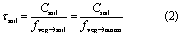
Our results show soil carbon losses in most regions where LUC has occurred in the last 150 years in the LCM simulations (figure 1). This is because in most regions pastures and croplands have increased at the expense of natural vegetation (figure S1 stacks.iop.org/ERL/12/084015/mmedia). This largely reduces the litter inputs to the soils due to less vegetation biomass in croplands and pastures compared to forests and also due biomass removal via crop harvesting (figure S2 and table 2). We find a global loss in soil carbon of 54.0 Pg C from the LCM simulations. The input-driven and turnover-driven changes contribute to a loss of 54.7 Pg C and 1.4 Pg C, respectively, while the synergy effects contribute a gain of 2.1 Pg C. A larger contribution to the spatial pattern of the total changes stems from the input-driven changes, as seen from the similarity of the patterns between the input-driven and total changes (figure 1). In some regions the input-driven and turnover-driven changes contribute in opposite directions to the total change. For most regions the synergy contribution is small.

Figure 1 Global separated soil carbon changes in kg C m−2 for the LCM simulations (including land management). The controls are obtained using equation (5) and taking the LCM_1860 equilibrium as the reference. (a) Total soil carbon changes, (b) contribution of the input-driven changes, (c) contribution of the turnover-driven changes and (d) the synergy effects.
Download figure:
Standard image High-resolution imageTable 2. Global carbon fluxes in absolute values and relative to the simulated net primary production (NPP) for the simulation including land management (LCM simulations in table 1).
| LCM_1860 | LCM_2005 | |||
|---|---|---|---|---|
| PgC yr−1 | % | PgC yr−1 | % | |
| NPP | 80.4 | 100 | 77.3 | 100 |
| Crop harvest | 1.6 | 2.0 | 3.6 | 4.7 |
| Wood harvest | 0.2 | 0.2 | 0.8 | 1.0 |
| Vegetation fire and herbivory losses | 6.6 | 8.2 | 6.1 | 7.9 |
| Litter | 72.0 | 89.6 | 66.8 | 86.4 |
| Soil respiration | 68.7 | 85.4 | 63.9 | 82.7 |
| Soil fire losses | 3.3 | 4.2 | 2.9 | 3.7 |
To understand the regional patterns of the input-driven and turnover-driven changes, we divide the globe into different regions based on where specific LUCs are dominant: afforestation, deforestation, and conversion of grasslands and pastures to croplands. Our results show a gain in soil carbon in most regions where afforestation has taken place, e.g. Central Europe and the East coast of USA, which stems from both the input-driven and turnover-driven contribution (figures 1 and 2). For some grid cells, despite the increase in forest cover (figure S1), the input-driven changes result in soil carbon loss. These are grid cells where the productivity of forests is lower than that of pastures, because the climatic conditions in these regions are not favorable for forest growth. Despite the differences in the climatic conditions, the turnover-driven changes always result in a gain in soil carbon that stems from the slower decomposition of woody litter compared to non-woody litter (figure 2).

Figure 2 Grid cell relationship between the input-driven changes and turnover-driven changes in kg C m−2 for the LCM simulations. To select the grid cells we calculated the difference in the cover fractions between the present-day and pre-industrial land cover and set a threshold of 10% for the specific dominant LUC.
Download figure:
Standard image High-resolution imageIn the deforested regions, where pastures and croplands have increased at the expense of forests, e.g. central USA and some parts of South America and Asia, we find both input-driven and turnover-driven soil carbon losses (figures 1 and 2). The input-driven losses are partly due to the decrease in productivity, which decreases litter inputs when forests are replaced with pastures or croplands, and in addition due to crop harvesting.
In regions where pasture or grasslands have been converted to croplands, e.g. some parts of Africa, the input-driven changes contribute to soil carbon loss, whereas the turnover-driven changes contribute to a gain (figures 1 and 2). The input-driven loss in these regions is mostly due to crop harvesting as the simulated productivity of grasslands and pastures generally does not differ much from that of crops in JSBACH (Nyawira et al 2016). The simulated turnover-driven gain in these regions mainly stems from the fire suppression on croplands (Andela and van der Werf 2014), which results in a global decline of the carbon losses due to fire (table 2). However, frequent fires may also lead to the conversion of burned biomass into organic matter that is richer in carbon and resistant to environmental degradation, which would lead to a slower turnover (Santín et al 2015).
The DGVM applied in our study has been shown to provide LUC emissions that are within the range of other model estimates (Le Quéré et al 2015). The global 54.0 Pg C soil carbon loss in our simulations lies in the middle of earlier estimates from a multitude of bookkeeping models and DGVMs, which span a large range from hardly any change to 105 Pg C (Houghton 2003, Reick et al 2010, Hansis et al 2015, Tian et al 2015). However, our results are not directly comparable to these estimates as we considered equilibrium states. The global present-day NPP of 77 Pg C in table 2 is larger than in other model estimates, which range between 53–72 Pg C (Rafique et al 2016). A comparison of the simulated NPP for the different PFTs reveals that JSBACH generally tends to be overproductive especially for forests (figure S3). While this may lead to biases in the simulated soil carbon for a given land-use distribution, biases in NPP often tend to cancel out when considering changes in soil carbon due to specific LUC (Nyawira et al 2016). Although there are no global data sets for the soil carbon turnover, the terrestrial carbon turnover obtained from different Earth system models in deforested regions show good agreement with observational-derived estimates, with model discrepancies occurring mainly outside the centers of LUC in the permafrost and dryland regions (Carvalhais et al 2014).
3.2. Spatial dependence of the controls on historical LUC
Vegetation productivity and decomposition rates vary depending on the climatic conditions; hence a key question arises: are the historically defined regions discussed above representative of the global response for the specific LUCs? To assess this we applied the separation approach to idealized LUC simulations. Here, the idealized simulations represent the response if all the grid cells in the globe were covered by one vegetation type that is then transformed to another vegetation type. We note that the idealized simulations do not include wood harvest for forests, because the harvest data is only available for realistic vegetation distribution.
The direction of the input-driven and turnover-driven changes for most regions in the idealized simulations matches our results for the dominant LUCs over the historical period. Afforestation on croplands and pastures results in a turnover-driven gain almost everywhere on the globe, while deforestation results in a loss (figures S4 and S5), which is in agreement with the results in figure 2. Exceptions occur in the dry and arid regions following a conversion of forest to cropland where fire suppression overcompensates for the effects of a shift from slowly decomposing woody to non-woody litter (figure S5). However, these regions have marginal forest cover in reality and have thus not been subject to substantial historical deforestation (figure S1).
Similar to the grid cells with historical afforestation, the direction of the input-driven changes following the conversion of pasture to forests varies depending on the region, whereas except for the marginal regions afforestation on croplands results in an input-driven gain (figure S4). The conversion of grasslands to croplands results in input-driven losses and turnover-driven gains in most regions where grasslands exist (figure S6). Overall, our results for the idealized simulations generally exhibit similar patterns as the regions considered in section 3.1; therefore, we can conclude that the simulated input-driven and turnover-driven changes for the dominant historical LUCs are qualitatively similar across different climate zones.
3.3. Contribution of land management
We apply the factor separation to the simulations excluding crop and wood harvesting for a comparison of the effects of land management on the controls with those of only the land cover change. Our results show a global loss of 22.4 Pg C in the LCC simulations (compared to 54.0 Pg C in LCM simulations). The differences in the total changes between the LCC and LCM simulations stem mainly from the input-driven changes (figure 3). Land management enhances the input-driven losses and decreases the gains almost everywhere in the globe, except for a few grid cells with afforestation where the input-driven gain is larger in the LCM simulations. The larger gain is due to the higher wood harvest intensity in 2005 compared to 1860, which amplifies the difference in the litter inputs in the LCM simulations, compared to the LCC simulations, as part of the harvest goes to litter (see section 2.2 and figure S8). Globally, we find an input-driven loss of 24.9 Pg C in the LCC simulations (compared to 54.7 Pg C in LCM simulations). The differences in the turnover-driven contribution between the LCM and LCC simulations are small. These differences are due to the different amount of woody litter through natural mortality when there is no harvest and due to the carbon losses through fire.
Figure 3 The difference in the (a) input-driven (b) and the turnover-driven changes in kg C m−2 between the LCM simulations and the LCC simulations. The differences are obtained by subtracting the input-driven and turnover-driven changes in figure 1 from those in figure S7. For the input-driven changes, negative values indicate that the carbon losses are larger without land management in regions where natural vegetation is converted to croplands or pastures, wheres the gains are smaller in afforested regions.
Download figure:
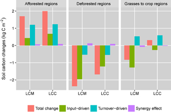
Standard image High-resolution imageOn average afforested regions exhibit larger soil carbon gain without wood harvest, while the deforested regions exhibit less losses due to larger litter fluxes in croplands (figure 4). In the regions with grasslands to croplands conversion, the turnover-driven gain associated with fire suppression outweighs the input-driven loss in the LCC simulations unlike in the LCM simulations. Hence in our model, crop harvesting overcompensates for the fire suppression effects in these regions.
Figure 4 Mean total changes in soil carbon in kg C m−2 and the contributing input-driven, turnover-driven and synergy changes. LCM represents the changes between the LCM_2005 and LCM_1860 simulations (including land management), while LCC represents the changes between the LCC_2005 and LCC_1860 simulations (excluding land management). The 'grasses to crop regions' also include regions where pastures have been converted to crop.
Download figure:
Standard image High-resolution image
The fraction of the NPP exported through harvest influences the relative contribution of the controls. Haberl et al (2007) estimate the NPP removed for food and timber, and forages consumed by livestock to be about 8.17 Pg C yr−1. In the LCM_2005 simulation, the biomass removed from the vegetation for crop and wood harvest is 4.4 Pg C yr−1 (table 2). Wood harvest contributes to about 0.97 Pg C yr−1 in the estimates by Haberl et al (2007), while in our simulations present-day wood harvest amounts to about 0.8 Pg C yr−1. Therefore, the larger difference between our simulated harvest and their estimate is likely due to the differences in the crop harvest or forages consumed by livestock that are not accounted for in the model. While the estimates by Haberl et al (2007) are based on harvest data, in the model one constant parameter is applied for all the grid cells in the globe for the fraction of crop biomass that is harvested versus left on site. This parameter is quite uncertain and may vary depending on the crop type (Nyawira et al 2016). Increasing the fraction of crop harvest would lead to larger global losses through the input-driven contribution.
Humans can manage soil carbon inputs through many ways, such as the choice of crop and tree species, fire management or residue management (see references in Erb et al 2016a). By contrast, except for tillage and ploughing on croplands, the effects of management on soil carbon turnover are more indirect, and occur through processes in the soils that control decomposition; the turnover-driven effects are thus less directly manageable than those related to input. Current projections show a higher land management intensity for present-day compared to pre-industrial land use. Global human population is projected to rise in the future, with the rise expected to cause a scarcity of productive land (Lambin & Meyfroidt 2011). As a result of this, land management on current ecosystems will most likely intensify to fulfill the increasing demand for food, shelter and livestock feeds. This will in turn decrease soil carbon inputs and enhance global soil carbon losses via the input-driven changes. With its substantial effects on the input-driven changes future LUC is likely to offset gains in soil carbon associated with climatic effects (Koven et al 2015).
3.4. Model limitations and the implications of missing processes
The YASSO sub-model captures the first-order dependence of soil carbon dynamics based on temperature and precipitation, as these are the measurable variables for the litter-bag experiments used in the parametrization of the decomposition rates. YASSO has been shown to provide estimates of litter decomposition and soil carbon storage without biases across the different climatic conditions (Tuomi et al 2009, Goll et al 2015). However, second-order effects associated with changes in soil moisture and soil temperature following LUC are not captured. Overall, it should be noted that the turnover-driven changes in our study are predominantly due to changes in the litter quality, but the PFT-dependent decomposition rates and fire effects additionally influence the simulated turnover.
In addition, land management practices other than crop and wood harvesting that influence the carbon turnover and the vegetation productivity are still missing in JSBACH. Tillage in croplands has been shown to increase historical carbon losses in other DGVMs due to the enhanced litter decomposition resulting from soil disturbances (Levis et al 2014, Pugh et al 2015). Although tillage amplifies the turnover-driven losses in these models, field observations still do not agree on its role in soil carbon cycling, with some studies showing that the adoption of no tillage does not significantly increase soil carbon stocks (e.g. Baker et al 2007).
Furthermore, our model does not represent the increase in crop productivity associated with fertilizer and manure application. However, increased crop productivity may not necessarily translate to higher litter inputs to the soils as most of the NPP is removed by crop harvesting. In addition, some studies show that in some regions the application of nitrogen fertilizers enhances decomposition and this effect counteracts the effect of added litter inputs associated with enhanced productivity (e.g. Russell et al 2009). As the relative share of the simulated input-driven and turnover-driven changes will be influenced by the inclusion of the missing processes, the results shown in our study may not represent the total LUC effects.
4. Conclusion
We have demonstrated how the factor separation approach can be used in assessing the relative contribution of the input-driven and turnover-driven controls on soil carbon changes after land-use change (LUC). On the global scale, we find that both the input-driven and turnover-driven changes have contributed to the changes in soil carbon associated with LUCs over the industrial era, with the input-driven contribution being larger than the turnover-driven contribution in our model. We find that crop and wood harvesting enhance historical soil carbon losses mainly through the input-driven changes. Thus, less management of current ecosystems is expected to reduce the committed soil carbon losses from past LUCs. Given that dynamic global vegetation models (DGVMs) differ widely in their representation of soil carbon dynamics, we encourage the application of this approach in other DGVMs and in model-intercomparison projects. This would facilitate a more robust quantification of the input-driven and turnover-driven changes and an assessment of the uncertainties associated with how different processes influence the controls.
Acknowledgments
We thank Gitta Lasslop for the valuable comments, which helped in improving the manuscript. We thank the two anonymous referees for the constructive comments, which have greatly improved the manuscript. We thank Martin Jung for providing us with the GPP data from which the NPP was derived. This work was supported by the German Research Foundation's Emmy Noether Program (PO 1751/1-1).