


Abstract
Identifying the drivers of global crop price fluctuations is essential for estimating the risks of unexpected weather-induced production shortfalls and for designing optimal response measures. Here we show that with a consistent representation of storage dynamics, a simple supply–demand model can explain most of the observed variations in wheat prices over the last 40 yr solely based on time series of annual production and long term demand trends. Even the most recent price peaks in 2007/08 and 2010/11 can be explained by additionally accounting for documented changes in countries' trade policies and storage strategies, without the need for external drivers such as oil prices or speculation across different commodity or stock markets. This underlines the critical sensitivity of global prices to fluctuations in production. The consistent inclusion of storage into a dynamic supply-demand model closes an important gap when it comes to exploring potential responses to future crop yield variability under climate and land-use change.
Export citation and abstract BibTeX RIS

Original content from this work may be used under the terms of the Creative Commons Attribution 3.0 licence.
Any further distribution of this work must maintain attribution to the author(s) and the title of the work, journal citation and DOI.
Corrections were made to this article on 4 May 2017. The style of the dashed line in Figure 3 was updated for clarity.
1. Introduction
The world market prices for food grains vary substantially on multi-annual and shorter timescales, with important implications for both importing and exporting countries. Although domestic markets are partially insulated from the world market [1], food prices particularly in developing countries can respond strongly to world grain prices [2]. Extreme increases in staple food prices, such as in 2007/08 and 2010/11 when world prices for wheat went up by more than 100% and more than 50%, respectively, in a matter of months, have been linked to far-reaching humanitarian crises and food riots in several developing and emerging countries around the world [3, and references therein]. For policies aimed at improving food security today, and in a future for which substantial changes in weather regimes and human land use patterns are expected, it is therefore important to understand the dynamics that drive short-term variations in world prices.
Weather fluctuations during plant growth render grain production inherently volatile from one growing season to the next. In particular, droughts and extreme heat spells have a large negative effect on cereal production around the globe [4], and severe droughts have also preceded the recent price spikes [5]. However, grain prices can also be affected by various other factors, and to which extent each of these factors contribute to price variability is a matter of ongoing research [e.g. 6]. Much of the recent debate about drivers of food price variability focuses on the price spikes of 2007/08 and 2010/11. Apart from direct effects of adverse weather events, several authors have ascribed a dominant role to export restrictions imposed by several important producer countries in response to yield shortfalls, further reducing world market supply and thus amplifying the price response to the yield shocks [5, 7, 8]. A similar argument has been made for the demand side, namely that importing countries, in response to an initial price rise, started to buy larger than usual quantities in an attempt to restock inventories and insure themselves against further price rises, thus collectively amplifying those very price rises [9–11].
On the other hand, increasing demand for biofuel production has been discussed as a major cause for rising prices particularly of maize and soybean, and partly of other crops due to substitution effects [12–14]. Finally, speculation by index funds driven out of the collapsing US housing and stock markets has been invoked as an external factor to explain the 'boom and bust' nature of the 2007/08 peak [15–17]. However, much of the existing analyses are descriptive (e.g. ref. [5] or rely on exemplary calculations (e.g. ref. [16] without attempting to reproduce the observed price time series in a quantitative way. A notable exception is a recent study that fits a supply-demand equilibrium model to 30 yr of grain price data, but explains the recent food price peaks based on cross-market speculation [17], without considering trade policies.
In this paper, we apply a global, annual supply-demand equilibrium model in order to quantify to what degree i) observed annual wheat price fluctuations over the last four decades can be explained by reported variations in production in the presence of dynamic storage; and ii) the remaining unexplained price variations in the last decade can be traced back to reported trade policy responses in the wheat market, as opposed to external drivers. We thereby offer a quantitative basis for assessing the vulnerability of the global food system to short-term production shocks, such as induced by weather.
A main characteristic of our model is that the supply function refers not only to current production, but includes supply from storage. Similarly, the demand function describes market demand by storage holders, not by end consumers. This integration of storage into the supply and demand functions permits a stock-flow consistent representation of short-term variability, in contrast to models that directly juxtapose production and final consumption (figure 1). We apply two different versions of the model: One in which final consumption is prescribed to match observed annual consumption (i.e. annual consumption is used as an input); it serves to quantify the price variability that is due to observed fluctuations in the physical quantities of supply and demand—that is, it includes any mechanisms that lead to changes in these physical quantities: weather or farm management affecting production; dietary shifts, substitution with other products, or changes in non-food uses affecting consumption (in particular, an increasing use of wheat due to rising maize prices related to biofuels would be included here); or even speculation, to the extent that it had any effect on actual production or consumption. In the other version, annual consumption is allowed to deviate from the observed long-term trend in response to simulated prices; it serves to quantify the amount of short-term price variability that can be explained solely by observed production changes.
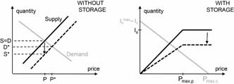
Figure 1 Schematic illustration of the supply and demand functions in an exemplary equilibrium model without storage (left), and in our model with storage (right; note that price is on the horizontal axis). In each case the implementation of a negative production shock is indicated by the arrow and the dashed supply curve. Assuming that supply and demand were in equilibrium before the shock (S = D), then shifting the supply curve by the amount that realized production S⁎ falls short of planned production S implies a new equilibrium price P⁎ at which demand D⁎ would exceed available supply S⁎ in the model without storage (left). In the model with storage (right), the supply curve represents total available goods including both new production and carryover stocks. Demand at the intersection can always be met, and the balance of goods is conserved through the producer-side and consumer-side inventories, Ip and Ic, respectively. Pmax,p is the price at which all producer-side stocks would be sold; Pmax,c the maximum price at which consumer-side storage is taken; and Imax,c the consumer-side 'target' storage level.
Download figure:
Standard image High-resolution imageThe effect of storage on the statistics of commodity prices has previously been investigated using the competitive storage approach (e.g. [18, 19]). In comparison, the model presented here is conceptually and computationally simpler, and explicitly designed to test the predictive capacity of the potential drivers of price variability discussed above. A more detailed comparison of our model and the competitive storage model can be found in the Appendix. We note that because of its simplicity, our model may be particularly suited for inclusion in an integrated assessment framework, where climate effects on short-term food price variations are considered alongside other economic and societal impacts of climate change and/or adaptation options. For example the sequencing of multiple climate-induced yield shortfalls, and the resulting depletion of stocks and rise of prices, would be overlooked on the 5-or 10-year time steps of conventional integrated assessment models, but can be accounted for with our model.
2. Methods
2.1. Data
We use world wheat (US hard red winter) production (supplementary figure S1 available at stacks.iop.org/ERL/12/054005/mmedia) and domestic consumption data (online supplementary figure S2) from the United States Department of Agriculture (USDA) Production, Supply and Distribution (PSD) online database2 as inputs to the model, and compare our simulated world ending stocks to data from the same source, and simulated prices to data reported by the World Bank3. Over the period 1975–2013, in the USDA PSD data, the cumulative difference between production and consumption exceeds the increase in stocks by approx. 100 mmt (million metric tons; see online supplementary figure S3). This inconsistency could be caused by missing or incorrect data in either or all of the production, consumption, and stocks time series. To obtain a self-consistent dataset for driving and evaluating our model, we eliminate the discrepancy by adding a constant amount of 2.7 mmt per year to the reported consumption data; assuming that consumption might be the most error-prone of the three datasets since its measurement is more indirect than that of production, and since systematic measurement errors in consumption may more easily go unnoticed than in stocks data which is cumulative. We note that this cross-the-board adjustment of the reported consumption data merely serves the purpose of this model study; we do not attempt an actual correction of the original data.
2.2. Model
The model presented here is designed to provide a simplified representation of year-to-year supply-demand dynamics, including stocks, on a global food grain market.
2.2.1. The short-term supply curve
Equilibrium prices on the agricultural commodity market are commonly modeled as the price at the intercept of a supply (subscript s) and a demand (subscript d) function of the type:


where Q is quantity, P is price, and e is price-elasticity4. The supply curve is generally considered to represent the marginal cost to producers of supplying an additional unit of e.g. grain; and the demand curve to represent the marginal price that consumers are willing to pay for an additional unit. This view corresponds to a long-term planning perspective where production can be adjusted along the supply curve to meet expected demand. Long-term changes in underlying conditions such as climate, consumer preferences, available production technologies, regulations, etc. can shift the supply and demand curves or change their shapes, leading to a new equilibrium price.
On annual or shorter timescales, however, producers have little capacity to adapt production: only to the extent that interhemispheric differences in growing seasons, or multiple growing seasons per timestep in a single region, allow them to change acreage or inputs in the second growing season in response to realized yields in the first growing season. A supply curve referring only to production therefore has very limited meaning at these timescales. Instead, the flexible part of supply comes from storage (grain inventories).
This has implications for how short-term production shocks can be accurately represented in a supply-demand equilibrium model. Previous studies have modelled such shocks by shifting the supply function by an amount corresponding to the production shortfall (or surplus) and thus obtaining a price shift [17, 20]. Except in the limit of extremely elastic demand, the quantity demanded at that new equilibrium price is, however, larger (smaller) than the quantity originally produced (figure 1, left); and because production cannot adapt, the difference would have to be supplied from (transferred to) storage. While this may be neglected when only looking at a single event, inconsistencies pile up from one shock to the next. Therefore, when an annual production time series is realized as a series of production shocks in an equilibrium supply-demand model, it is important to keep track of storage as an integral part of total supply.
We include storage directly into the supply curve. When the supply curve is reinterpreted to refer not to long-term production potential but to a given year's realized production plus carryover stocks, then it has a defined upper bound: At any given point in time, no more goods can be supplied than the sum of goods just harvested and those left in storage from previous harvests. We introduce a variable Ip representing total producer-side storage, or inventories, which may be thought of as the sum of grain held by storage firms, farmers, or in any other stores before being sold on the world market. Assuming that any new harvest is added to this aggregate storage term, the storage balance is:

where t is the present time step (year), Qx is the quantity sold to the consumer side, and H is production (harvest). We then define the short-term supply function as
where the index p denotes the producer side; P is world price; and Pmax,p is the (hypothetical) price at which all existing stocks would be sold (figure 1, right). The exponent α controls the shape of the supply curve, and can be interpreted as a short-term elasticity of supply; α = 1 corresponds to a linear supply curve, whereas larger (smaller) values of α correspond to a convex (concave) shape of the supply curve. δtrade is the fraction of total producer-side stocks that is available for trade. For the present application, we set δtrade = 1 except during export restrictions; see Results.
With this type of supply function it becomes possible to consistently model a series of production shocks, or more generally a variable production timeseries H(t). According to equation (3), any change in H leads to a change in Ip, shifting the upper bound and thus stretching or compressing the entire supply curve. Because the carryover stocks are also part of Ip, the balance of goods is conserved from one time step to the next.
2.2.2. The short-term demand curve
Similar arguments can be made on the demand side. End consumers of staple foods typically do not buy directly on the world market, but are at the end of a supply chain including wholesale, processing, and retail enterprises most of which keep some amount of their inputs and/or outputs in storage [21]. Governments also store food grains over longer periods of time as strategic reserves. On long timescales, variations in all these grain stocks may cancel out, and the demand curve can be seen as an expression of the end consumers' willingness to pay for a given product or its derivatives. On short timescales, however, the world market price forms on the basis of the demand actually registered by market participants, e.g. large grain vendors, governments, etc. Their demand is an expression of their willingness to store grain at a given moment, and then process and/or resell or distribute it later.
Analogous to the producer side, we assume that the consumer-side storage level Ic is given by

where Qx is the quantity purchased on the world market (equal to the quantity sold by the producer side), and Qout is final consumption. We further introduce a maximum storage level Imax,c that controls the upper end of the short-term demand curve, such that at very low prices, the consumer side will buy just enough grain to refill their storage Ic to the level Imax,c. The interpretation of Imax,c is not necessarily the maximum physical storage capacity, but rather a measure of the amount of storage that consumers consider optimal. The demand function is then in the simplest form given by
where Pmax,c is the maximum price consumers are ready to pay for a single unit (figure 1, right). The exponent β controls the shape of the demand curve, and can be interpreted as a short-term price elasticity of world market demand.
We investigate two different versions of the model: One (called FixCons, for fixed consumption) in which final consumption Qout is prescribed to match observed annual consumption; and one (called FlexCons, for flexible consumption) in which annual deviations from the observed long-term consumption trend are determined within the model based on simulated prices, according to

with  . That is, we assume that if the world price in year t is equal to the average price of the τ previous years, consumption lies on the long-term trend line (Qout,ref is the 11 yr running average of reported annual consumption, online supplementary figure S2). If the price is higher (lower), consumption is below (above) the long-term trend, with ed < 0 being the price elasticity of consumption (different from the elasticity of demand of the consumer-side storage holders, β). Equation (7) is a highly simplified representation of final consumption that assumes that consumers adapt to long-term (as defined by τ) price changes, but are sensitive to short-term fluctuations. Insulation of domestic markets is only taken into account through the constant elasticity ed, neglecting changes over time in the transmissivity between world and domestic markets (and neglecting differences between different national and regional markets, which are all lumped together in this global model). This simple approximation serves the purpose of the present study, but we note that it could very easily be replaced by different, more sophisticated representations of Qout.
Given these supply and demand functions, we assume market clearance in each time step, i.e. Qd(t) = Qs(t) = Qx(t) , and thus obtain the equilibrium price P(t) and the quantity traded Qx(t) from equations (4) and (6). Note that in the present application of the model we make the simplifying assumption that all international trade is conducted at a single world market place between one representative producer and one representative consumer, and that we do not take into account any specifics of futures versus spot markets. The model described here may be extended, e.g. by modelling the global supply curve as the sum of individual supply curves representing multiple independent market participants, but is here deliberately kept as simple as possible, in order to explore the effects of the most basic supply-demand and trade mechanisms.
We point out that our modeling approach does not explicitly account for any particular costs or profits incurred by storage holders on the producer or consumer side. Instead, the supply and demand functions represent the aggregate behavior of storage holders, which follows from their respective objectives (e.g. profit maximization), characteristics (e.g. risk aversion), and costs incurred (e.g. for production and storage). Our rationale is to avoid modeling each of these factors explicitly—both because of the resulting complexity and because objectives, characteristics, and costs may differ substantially between different types of private and public storage holders—and instead choose a simple but plausible set of aggregate supply and demand functions. In particular, a potential effect of storage costs is implicit in the concave form of the supply function (α < 1, i.e. producer-side storage holders sell relatively much grain even at low prices).
The model workflow within a given timestep is illustrated in online supplementary figure S4. The model is implemented in Python; the program code is available upon request.
2.3. Model parameters
Parameter values used in this study are given in table 1. The consumer-side maximum storage capacity Imax,c is set to 190 mmt (55% of 1975 consumption) above the long-term average annual consumption:
where  is the running average consumption (we use an 11 yr window centered on the year in question), and Imax,c,+ is set to 190 mmt. That is, consumers collectively desire to hold up to 190 mmt as excess stocks, in addition to basic working levels. The ratio of Imax,c,+ to average annual consumption (the 'target' consumer-side stocks-to–use ratio) thus declines from 55% in 1975 to about 30% in the 2000s. This range appears plausible because it is somewhat higher than the actual historical range of about 15%–40% for the global stocks-to–use ratio [22]. The total storage level is initialized with 80 mmt at the beginning of the simulation, to match reported ending stocks of 1974. The demand curve is assumed linear, β = 1, as the simplest choice for this parameter. The remaining parameters Pmax,c, Pmax,p, and α are chosen to obtain a good match of the simulated price time series with the observed one. Systematic variation of the parameters shows that they control the average price level as well as the overall amplitude of price variability, but have no major effect on the relative magnitude of individual price changes; i.e. the shape of the price time series is insensitive to changes in these parameters apart from scaling (online supplementary figure S5). Our parameter estimates are further corroborated by an ad-hoc application of the model to corn (maize), which yields a considerable agreement between simulated and observed price variations using the same set of parameter values as chosen for wheat; see the Appendix.
Table 1. Data and parameter values used in simulations with prescribed (FixCons) and endogenous (FlexCons) annual consumption.
| Symbol | Description | FixCons | FlexCons |
|---|---|---|---|
| Exogenous (data from USDA) and endogenous variables | |||
| H(t) | Annual production | exog. | exog. |
| Qout(t) | Annual final consumption | exog. | endog. |
| P(t) | Annual price | endog. | endog. |
| Ip(t) + Ic(t) | Annual total ending stocks | endog. | endog. |
| Producer side parameters | |||
| α | Exponent of supply curve | 0.1 | 0.1 |
| Pmax,p | Producers' maximum price ($) | 350 | 350 |
| Consumer side parameters | |||
| β | Exponent of demand curve | 1.0 | 1.0 |
| Pmax,c | Consumers' maximum price ($) | 850 | 850 |
| Imax,c,+ | Consumer storage capacity in excess of annual demand (% of year–1975 demand) | 55 | 55 |
| ed | Price elasticity of final demand | — | −0.1 |
| τ | Price adjustment timescale of consumption (number of previous years to compute reference price) | — | 3 |
aThe endogenous calculation of annual final consumption is based on the long-run consumption trend, which is determined exogenously from annual USDA data; cf equation (7).
The parameter values for the FlexCons model are the same as for the FixCons model, except that two additional parameters enter through the representation of final consumption, equation (7): the price elasticity of final consumption, ed, and the number of previous years τ over which prices are averaged to obtain the reference price Pave. The larger τ, the slower are consumers to adapt to changing price levels. Both parameters are used to fit the model to observed consumption anomalies. The result is consistent with observations on a multi-year scale, even though in individual years simulated anomalies can differ from reported ones in magnitude and sometimes in sign (online supplementary figure S6), as may be expected from this simplified representation which neglects e.g. further price effects with different lag times, spatial and temporal differences in price transmissivity, and confounding factors present in the reported data, such as substitution effects with other food commodities. The value of −0.1 for ed is similar to the domestic short-run elasticity of −0.11 estimated by [5] for the USA during the 2007/08 price spike.
The FlexCons model is first run with constant year–1975 input data for a number of time steps until a stationary price is reached, and then with varying input from 1975–20165. The sensitivity of the model to variations in the different parameters is shown in online supplementary figures S7 to S13. We note that the calibration of the model—adjusting the free parameters to find the best match with observed data, as described above—was performed (jointly for the FixCons and the FlexCons model) only on the period 1975–2013. The years 2014–2016 were only added to the analysis once the parameters had been fixed at the values reported in table 1. This extension thus serves as an out-of–sample test of the model calibration. Together with the application to corn in the appendix, we therefore offer two types of 'out-of-sample' tests (across time and across crop types) to lend support to the model formulation and parameter estimates.
3. Results
3.1. Supply-demand dynamics
We first run the FixCons model (consisting of equations (3) through (6)) time-forward with annual global wheat production and consumption from 1975 to 2016 taken from reported data. Results are shown in figure 2 (violet lines). Given that both annual production and consumption are prescribed, the FixCons model matches reported storage almost perfectly by design. Notably, the variations in price are also captured to a large extent by this production-consumption driven model (figure 2, bottom); the Pearson correlation coefficient is 0.81. The agreement of simulated with observed annual prices is similar to a previous model study for 1982–2010 [17], but the advantage of our model is its consistency: production, consumption and storage all match reported values, and the difference between production and consumption is precisely balanced by storage changes and thus carried forward through the simulation (stock-flow consistency).
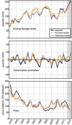
Figure 2 Model results for wheat. Global, annual stock levels (top), consumption anomalies with respect to the 11 yr running average (middle), and world market price (bottom). Annual consumption anomalies are prescribed from data in the FixCons model version (violet) and computed endogenously in the FlexCons model version (orange). Black lines show reported values. Annual price data (black line in bottom panel) are aggregated from reported monthly data as averages from July of the year indicated to June of the following year, to represent crop years rather than calendar years. The difference between the black and violet lines in the middle panel is due to the offset of 2.7 mmt per year added to reported consumption values to match reported stock variations (see main text and supplementary figure S1). The grey shading indicates the 'out-of-sample' validation period 2014–2016 which was added after the calibration of model parameters.
Download figure:
Standard image High-resolution imageA key parameter of this model is the 'target' inventory level of the consumer-side representative storage holder, Imax,c (see figure 1). That is, in the limit of very low prices, the storage holder would buy enough grain to fill their inventories up to this level, to safeguard against future price rises. We find that the overall downward trend in real prices since the 1970s can only be reproduced if this target level is assumed to decline, relative to average consumption (supplementary figure S5). This assumption is consistent with the observed decreasing trend in public stock-keeping, only partially being compensated by private stocks [21].
Our model also offers an opportunity to further decompose the different contributions to annual price variability. If annual-scale variability in consumption is eliminated by prescribing each year's final consumption to the 11–year running average of observed consumption, the simulated price and stocks series are somewhat shifted but most year-to–year variations in both stocks and prices are still reproduced (online supplementary figure S14). This indicates that the dominant portion of annual-scale variability in prices and stocks is due to variability in production; consistent with the greater amplitude of variability in production than in consumption (see online supplementary figures S1 and S2). On the other hand, the importance of dynamic storage in reproducing past price changes is illustrated in a scenario where storage is artificially kept fixed, i.e. no surplus or deficit is carried over into the next years storage (figure 3). Results are inferior to the model with dynamic storage both in terms of the overall price trend and in terms of the magnitude and direction of price change in many individual years or episodes. In particular, price peaks often begin too early, pointing to the missing buffer effect of storage.

Figure 3 Fixed-storage scenario. Solid lines are as in figure 2 (top and bottom panel). Dashed lines show results of a simulation with the FixCons model where stocks are, at the end of each agricultural year, reset to their starting value. Thus, while annual changes in production and consumption still get reflected in Ip and Ic, and thus, in the price, no surplus or deficit is carried over into the next year's storage.
Download figure:
Standard image High-resolution imageIn order to isolate the part of annual price variability that is driven by changes in annual production, and to exclude any other potential drivers, we now relax the observational constraint on consumption. Only the long-term trend (11 yr moving window) of consumption is prescribed, to ensure long-term balance of production and consumption; the drivers of this trend, such as population growth or long-term changes in diets, are assumed unrelated to short-term price fluctuations. Actual consumption in each year is computed internally through a simple iso-elastic relation with the simulated price anomaly (equation (7)).
The resulting 'FlexCons' model (orange lines in figure 2) matches reported prices similarly well as the FixCons model, with a Pearson correlation coefficient 0.88. In addition, variations in stock levels as well as consumption are also largely reproduced. Systematic variation of the different parameters shows that the basic shape of the model results is rather insensitive to the exact choice of parameters (supplementary information). Within the bounds of parameter uncertainty, this model thus provides a self-consistent estimate of the effect of production variability on grain prices, excluding any other short-term effects such as cross-market speculation, or rapid demand-side responses to biofuel policies or prices of other commodities.
We note that since annual production is taken from data, the model does not control for the feedback of previous prices on production through farmers adapting acreage and farm inputs. Here we only explore the effect of production on prices. We also point out the consistent prediction of price and stocks trends during 2014–2016 in both model versions, which lends support to the parameter values estimated for 1975–2013. Moreover, statistical properties (autocorrelation and skewness) of reported annual prices are closely reproduced by our model (table 2).
Table 2. Descriptive statistics for annual wheat price timeseries 1975–2013.
| Autocorrelation | ||||
|---|---|---|---|---|
| lag 1 | lag 2 | lag 3 | Skewness | |
| With trend | ||||
| Observed (World Bank) | 0.86 | 0.72 | 0.70 | 1.03 |
| FlexCons model |
0.85 | 0.74 | 0.68 | 1.17 |
| Detrended |
||||
| Observed (World Bank) | 0.32 | −0.31 | −0.36 | 0.42 |
| FlexCons model |
0.29 | −0.13 | −0.36 | 0.39 |
| FlexCons model, randomized production |
0.28 | −0.02 | −0.13 | 0.12 |
adriven by reported production and consumption values, as described in main text, and without trade policies bremoving 11 yr running mean from observed and simulated price series before calculating autocorrelation cdriven by a 5000 yr long random sample based on the observed production distribution. No trade policies
3.2. Trade policies
The model (in both the FixCons and FlexCons versions) overestimates wheat prices in the late 1990s and early 2000s—especially in 2003—while underestimating them from 2007 on, and especially after 2009. This is in agreement with previous studies that found that prices during these times are difficult to explain based solely on actual production and consumption. Because our model explicitly includes storage, we can represent, in a simplified fashion, two mechanisms that have been proposed as potential drivers of recent food price spikes, and in fact also of the missing spike in 2003: Export restrictions and import policies.
Table 3 shows a summary of major trade policy events that have been cited in relation to recent wheat price variability. These fall into two categories: Export restrictions by major wheat producing countries; and changes in stock-holding and import policy by large consumer countries. We first consider the latter, demand-side policies. A potential driver particularly of the price rise in 2010 and 2011 has been identified in 'aggressive' buying strategies of several importing countries, which attempted to restock their inventories in reaction to initial price rises and in expectation of continuing high price levels [9]. Conversely, the period between 2003 and 2007 was marked by low world wheat stocks, due largely to significant stock reductions in China, whose wheat exports began rising in the 1990s and spiked in 2003 and 2006/2007 (online supplementary figure S15).
Table 3. List of largest wheat producing and consuming countries (by volume in 2013; producing countries listed make up ca. 80% of world production; respective share of world exports/imports shown in brackets, with largest exporter/importer in bold; source: USDA) and major trade policy events since the year 2000.
| Countries | |
| Producer | EU (19%), China (0.5%), India (4%), USA (19%), Russia (11%), Canada (14%), Australia (11%), Pakistan (0.5%), Ukraine (6%) |
| Consumer | China (4%), EU (2.5%), India (0%), USA (3%), Russia (0.5%), Pakistan (0.3%), Egypt (6%), Turkey (2.5%), Iran (3%) |
| Trade policy events | |
| 2000–2007 | China: Historically large exports, peaking in 2003 and again in 2006-07; stocks reduce from 100 mmt in 2000 to 40 mmt in 2003 (USDA; supplementary figure S15) |
| 2007 | Export restrictions/bans India, Russia, Ukraine, Argentina, Kazakhstan [5] |
| 2010 | Export ban Russia [9] |
| 2011 | Unusual purchases by China, Indonesia, Egypt, and other North African and Middle East countries; EU, Russia, Turkey lift import levies [9] |
We represent these major changes in consumer-side buying/selling behaviour as changes in the consumer-side 'target' inventory level, Imax,c. As a simplified representation of China's major reduction in inventories, we gradually reduce Imax,c by up to 8% between 2000 and 2006 (see figure 4, inset in top panel)6. This figure should not be too large given the fact that China's share of the global wheat stock was about 40% in 2000, but had dropped to about 20% by 2004 [23].
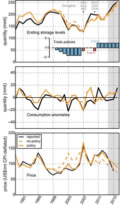
Figure 4 Results for the FlexCons model with trade policy changes starting in year 2000. Trade policy scenarios include reduced or enhanced demand by importing countries, or reduced exports by producing countries (inset in the top panel; blue and red bars show the fraction by which Imax,c and δtrade, respectively, are reduced or enhanced; see main text). Grey triangles and country acronyms mark major drought events which led to shortfalls in wheat production and likely triggered the ensuing trade policy responses [5, 9]. Results without trade policy changes are shown for comparison (dashed lines).
Download figure:
Standard image High-resolution image
Chinese exports then stopped rising in 2007 and sharply dropped in 2008. We assume that in the light of the emerging food price crisis, any efforts to reduce nationals stocks were presumably halted, and therefore reset Imax,c to its baseline value during 2007–2010. In the wake of the 2010/11 price spike, surging wheat purchases by many importing countries were reported, which were interpreted as attempts to restock inventories. As a simplified representation of these policy changes, we raise Imax,c to 5% above the baseline from 2011 onwards.
Restrictions placed on wheat exports by several important producer countries have been suggested as another possible driver contributing to the wheat price rises in 2007/08 and 2010/11. Just as consumer countries' precautionary imports, these restrictions are widely regarded as policy responses to concurrent or anticipated supply shortages, related to severe droughts in Australia, India, and Ukraine before and during 2007/08, and in Russia, China and the USA during 2010/11, that reduced wheat harvests [5, 9]. Specifically, export restrictions or bans were effective in Argentina, Russia, Ukraine, Kazakhstan, and India for part or all of the period between late 2006 and early 2008. Russia again banned wheat exports in 2010.
Seen from a world-market perspective, export restrictions effectively make a part of the total supply unavailable for international trade7. In our model, this can be represented by temporarily withholding part of the producer-side stocks from the world supply function. As a simplified representation of the reported export restrictions or bans described above, we reduce the fraction of producer-side stocks available for trade, δtrade, to 0.97 in 2007 and 2010 (with δtrade = 1 in all other years; cf equation (4). I.e. we assume that 3% of global producer-side stocks are unavailable to international trade in 2007 and again in 2010, whereas at other times all stocks can be traded. These numbers are likely no overestimation given that the countries which banned or restricted exports during the 2007/2008 price spike together made up about 25% of world exports [5].
Model results with these trade policy measures are shown in figure 4 for the relevant period. Compared to the case without trade policies, observed prices since 2000 are matched much more closely. In particular, the simulated peak in 2003 is greatly reduced, and substantial price rises are now simulated in 2007 and 2010. We also find an improvement in simulated storage and, in some years, consumption, during these periods. While without trade policies, ending stocks were overestimated during 2000–2006, they are now closely reproduced, and the underestimation after 2009 has also been reduced. The pronounced negative consumption anomalies in 2007 and 2010 are now reproduced as well (figure 4, middle). The fit is not perfect; notably, consumption is still too high, and therefore stocks too low, in 2008 and 2009, hinting at the limits of our simple representation of annual consumption in the FlexCons model. Nonetheless, these results demonstrate that a substantial portion of observed variability can be explained on the basis of production changes and idealized representations of trade policy changes, without accounting for any other potential drivers.
4. Discussion and conclusions
We have presented a simple model of global, annual grain supply and demand that incorporates storage into the supply and demand functions. We have applied the model to the recent four decades of wheat supply and demand, and demonstrated that a substantial part of the observed annual price variability can be explained solely by variations in production and resulting changes in storage and consumption. To our knowledge, this is the first attempt at reproducing such a long section of observed prices with a stock-flow consistent quantitative model.
The inclusion of dynamic storage not only ensures stock-flow consistency but also substantially improves the simulation of historic year-to–year price changes, especially when it comes to the timing of price peaks, as illustrated by a scenario with fixed storage. In addition, the representation of storage in the model makes it possible to account for mechanisms like export restrictions and import policies, and we have demonstrated that these mechanisms, together with the production shocks that likely triggered them, can explain a large part of the recent observed price variability including the major peaks in 2007/2008 and 2010/2011. Our study is thus the first to reproduce this period of enhanced price variability within a simple supply-demand model.
We note that both the model—in particular, the representation of final consumption—and the trade policy scenarios applied above may be refined, potentially improving the fit of the model to reported data. On the other hand, we do not expect a perfect fit. Mechanisms that were intentionally neglected here, such as interactions between the wheat market and other markets, likely did play a role in past wheat price variations, and can be expected to explain at least part of the remaining discrepancies between model and data. The present study merely shows that those factors may not have been of primary importance on the annual timescale. In particular, while speculation does not seem to play a major role for annual prices, it may be expected to have a larger effect on monthly or shorter timescales.
In our simulations we have assumed that all of the reported wheat production and consumption is available for trade on a global market (except when we applied export restrictions). In reality, at any given time many producers and consumers will be isolated from the world market, be it due to policy regulations, infrastructure, or other barriers or preferences. Of the four most important food grains wheat, maize, rice, and soybeans, the fraction traded internationally is greatest for wheat (about 18% during the 2000s), and smallest for rice (about 7%) [24]. However, the amount that is available for international trade cannot simply be inferred from realized trade (reported exports and imports), since the latter is a function of price; thus our simplifying assumption of 100% availability. Price in our model is in fact invariant with respect to proportional changes in quantity supplied and demanded, as long as Imax,c is also changed proportionally, and the changes are applied uniformly over the simulation period (see equations (4) and (6)). That means, for example, consistently considering only half of the reported production and consumption amounts would not change the simulation results. Conversely, changes over time in the fraction of total production and/or consumption available for international trade do affect results, as we have demonstrated for the trade policy scenarios.
We also note that in reality, there is not always a clear distinction between producer-side and consumer-side storage. In our model, stocks move from producer-side to consumer-side storage as soon as they are sold on the world market; applied to the real world, that would mean that depending on the ownership and on the owner's intended use, a particular quantity of grain in some storage facility may be considered either as producer-side or consumer-side stock, no matter where it is physically located. The distinction is however a useful modelling concept, because it allows storage to buffer price movements on both sides of the market. It is important to realize that the short-term price elasticity of world market demand is higher than just that of the—relatively inflexible—final demand (just as the short-term price elasticity of world market supply is higher than that of farm-level production); and that this price elasticity depends on storage. This fact is reflected in our model formulation.
Our results enable a quantitative review of previous, qualitative explanations of recent grain price variability. They suggest that cross-market mechanisms, such as speculative demand moving into the wheat market as other markets collapsed, may not be critically necessary for explaining the observed sharp rises in annual world prices, but may, when present, rather have further amplified the already substantial price excursions caused by supply-demand mechanisms. This would also imply that production shocks, together with protective responses of grain market participants, have a potential of sparking price spikes large enough to seriously threaten food security. This makes potential future increases in yield variability due to climate change [25, 26] a particular concern.
Beyond the present results, our model offers multiple opportunities for future research. For example, it may be particularly interesting to combine the model with crop growth and macroeconomic models to assess the food security and livelihoods implications of different climate change, agricultural management, and policy scenarios.
Acknowledgments
The authors wish to thank James Vercammen, Matthias Kalkuhl, and Yaneer Bar-Yam for helpful discussions. The work was supported within the framework of the Leibniz Competition (SAW-2013 PIK-5). The publication of this article was funded by the Open Access Fund of the Leibniz Association.
Appendix: comparison with competitive storage approach
The effect of storage on commodity prices has previously been modelled using the competitive storage approach [18, 27–29] or cobweb-type models [30, 31]. Both approaches have been applied to random supply shocks and are able to reproduce many statistical properties of observed price series. The competitive storage model was, in a refined version, also applied to actual historical wheat supply and demand data, and shown to reproduce the approximate shape of the historical price series, though not the magnitudes of the price changes [19]. The model presented here is conceptually and computationally simpler than the competitive storage model, and explicitly designed to enable a quantitative review of the potential drivers of price variability discussed above.
The competitive storage model is derived from the assumption of profit-maximizing speculative behavior by a risk-neutral storage holder (agent) [29]. The representative agent is assumed to be a 'price-maker', that is, their own storage decision in a given time step influences their expectation of the next time step's price. The agent takes storage only if the expected future price is higher than the current price (arbitrage condition). In comparison, in our model, the representative producer agent behaves like a 'price-taker', i.e. their future price expectation (expressed by the parameter Pmax, p) does not depend on their own storage decision (and, in the basic model version examined in this paper, is in fact constant). This also means that it does not strictly observe the arbitrage condition when compared with the actual price series8: storage is often or always taken even in years that are followed by decreasing prices.
Thus, the representative agent in our model does not behave like a single profit-maximizing speculator with rational expectations. However, observed global prices and stocks do not, either: substantial stocks are carried through even when prices are falling (e.g. compare the black lines in the top and bottom panels of figure 2). The rationale behind our model is that the representative agent should approximate the collective behaviour of the numerous actual storage holders, which in reality may not all follow the same objectives and have access to the same information. In particular, while some (e.g. large commercial storage firms) may come close to the theoretical, profit-maximizing, price-making speculator with rational expectations, others may be too small to have a discernible influence on world price [32], or may have non-commercial objectives (e.g. strategic reserves), or may require minimum working stocks (e.g. processing industry). Far from explicitly including all these cases, we show here that a simple and transparent global model with plausible assumptions about supply and demand functions can reproduce their collective behaviour rather closely. This is not only true for the annual values of price, storage, and consumption, as shown above, but also for statistical properties like autocorrelation of prices (table 2), which are reproduced by our model with a similar accuracy as by a recent application of the competitive storage model [19].
We note that our model can be extended: e.g. rather than keeping Pmax,p constant, it may be set to increase with decreasing stocks, thus reflecting the behavior of 'price-makers'. Moreover, the model could at little computational cost be extended to multiple agents, whose parameters could then be chosen to reflect different types of behavior. It is therefore a simple and transparent tool for exploring various supply- and demand-related effects on prices, complementing more sophisticated methods like the competitive storage model.
Illustrative application for corn (maize)
As a form of 'out-of–sample validation', we apply the FixCons model to corn (online supplementary figure S16), using the same set of parameter values as chosen for wheat (table 1). While simulated prices are generally too high, annual price variations (difference over preceding year) are already in considerable agreement with observations, and the Pearson correlation between simulated and reported prices is 0.71. In fact, one may expect the values of Pmax,p, Pmax,c, and Imax,c to be different for different crops, since there is no reason why average prices and target storage levels should be identical across different crops. Adjusting these crop-specific parameters would likely improve the model's fit to observed corn prices. We note here that the fact that much of the corn price variability is reproduced even without adjusting any parameters, lends support to the model structure and the values chosen for the more internal parameters, α and β (which are related to the behaviour of the storage holders and may depend less on the specific crop).
Footnotes
- 2
https://apps.fas.usda.gov/psdonline/, last accessed on 17 January 2017
- 3
http://data.worldbank.org/data-catalog/commodity-price-data, last accessed on 17 January 2017
- 4
Besides this iso-elastic form, other functional forms are sometimes used, e.g. a linear form, Q ∝ e P.
- 5
Since data refer to agricultural years, the ending storage level and consumption for year 2016 are in fact forecasts, as of 17 January 2017, by USDA for the agricultural year 2016/17. For the same reason, no observed price is available for 2016 (i.e. the agricultural year 2016/2017), and the correlation coefficients between simulated and observed prices reported below refer to the period 1975–2015
- 6
Note that exports are not a direct indicator of changes in stock-holding policy, since they depend also on prices. We only use major shifts in Chinese exports and stocks as a motivation for our simple policy scenario, assuming that they are too large to be just market responses to price signals, and seeing as exports peaked during times of stable and low world prices. A more realistic scenario may be designed based on analysis of reported policy changes in China and other countries, but in the present study we explore the effects of this simple and transparent approximation.
- 7
They also reduce demand on the world market as some or all of the demand in the restricting country is satisfied through domestic supply. However, for major exporting countries, the net effect of an export restriction will still be a reduction in world market supply relative to world market demand.
- 8
Note, however, that it does observe the arbitrage condition internally: No storage is taken if current price is above the expected future price, Pmax,p. The difference is in how the price expectation is formed.