
Abstract
The discrepancy between recent observed and simulated trends in global mean surface temperature has provoked a debate about possible causes and implications for future climate change projections. However, little has been said in this discussion about observed and simulated trends in global temperature extremes. Here we assess trend patterns in temperature extremes and evaluate the consistency between observed and simulated temperature extremes over the past four decades (1971–2010) in comparison to the recent 15 years (1996–2010). We consider the coldest night and warmest day in a year in the observational dataset HadEX2 and in the current generation of global climate models (CMIP5). In general, the observed trends fall within the simulated range of trends, with better consistency for the longer period. Spatial trend patterns differ for the warm and cold extremes, with the warm extremes showing continuous positive trends across the globe and the cold extremes exhibiting a coherent cooling pattern across the Northern Hemisphere mid-latitudes that has emerged in the recent 15 years and is not reproduced by the models. This regional inconsistency between models and observations might be a key to understanding the recent hiatus in global mean temperature warming.
Export citation and abstract BibTeX RIS

Content from this work may be used under the terms of the Creative Commons Attribution 3.0 licence. Any further distribution of this work must maintain attribution to the author(s) and the title of the work, journal citation and DOI.
1. Introduction
Despite increasing radiative forcing, the observed globally averaged annual mean surface temperature (Tmean) has only increased very slowly since the late 1990s (e.g., IPCC AR5 2013). This phenomenon has often been referred to as the global warming hiatus (Meehl et al 2011). Several studies (e.g., Fyfe et al 2013, Fyfe and Gillett 2014, England et al 2014) have shown that recently performed climate change simulations do not reproduce the global warming hiatus. Possible causes for this mismatch that have been discussed in the recent literature include decreases in stratospheric water vapor (Solomon et al 2010), increases in stratospheric and tropospheric aerosol concentration (Solomon et al 2011, Kaufmann et al 2011) and internal climate variability manifested via La-Niña-like decadal cooling in combination with a vertical re-distribution of heat in the ocean (Meehl et al 2011, 2013, Balmaseda et al 2013, Kosaka and Xie 2013, England et al 2014).
While discussion has focused primarily on globally averaged Tmean, climate change and its consequences are often associated with climate extremes occurring at regional scales (Seneviratne et al 2012). Recently, Seneviratne et al (2014) have shown that hot extremes have continued to warm despite the global warming hiatus. However, apart from this study, little has been said about temperature extremes in the global warming hiatus discussion. In this paper, we therefore consider observed and model-simulated changes in temperature extremes over recent decades at global and regional scales and investigate the extent to which observed features are reproduced in the model simulations that were contributed to the Coupled Model Intercomparison Project Phase 5 (CMIP5, Taylor et al 2012). We will focus on exploring the following two questions: (a) are the observed and simulated trends significantly different from zero and (b) are the observed trends consistent with the simulated range of trends for the past four decades (1971–2010) in comparison to the recent 15 years (1996–2010) representing the warming hiatus period.
2. Data and methods
We use the HadEX2 global gridded observational dataset of temperature and precipitation extremes, which is documented in detail in Donat et al (2013) and is available from the CLIMDEX project website (www.climdex.org/). This dataset is based on climate extremes indices as defined by the Expert Team on Climate Change Detection and Indices (ETCCDI) (Zhang et al 2011). The ETCCDI indices remain currently the only source of publicly available information about observed temperature and precipitation extremes in many parts of the world.
Here we focus on two widely used ETCCDI temperature indices, the temperatures (in °C) of the coldest night (TNn) and warmest day (TXx) of each year (e.g., Zhang et al 2011, Seneviratne et al 2012). We investigate the changes in these extreme temperature indices over the most recent 40 years (1971–2010) available from HadEX2. These indices have also been calculated for a large set of CMIP5 models (Sillmann et al 2013a) and are available from the ETCCDI extremes indices archive (www.cccma.ec.gc.ca/data/climdex/). We use 27 CMIP5 models (see online supplementary table S1 available at stacks.iop.org/ERL/9/064023/mmedia) and all available ensemble members for each model for which daily minimum and maximum near surface temperatures and daily precipitation accumulation were available for both the historical and scenario simulation. The historical simulations from 1971–2005 are concatenated with simulations using the RCP4.5 forcing scenario (Thomson et al 2011) to cover the analysis period. Indices from the models were interpolated to the 3.75° (longitude) × 2.5° (latitude) grid of the HadEX2 dataset to facilitate comparison. Furthermore, a mask was applied to all models and HadEX2 to exclude regions where HadEX2 data coverage is insufficient (i.e., where annual indices were available in fewer than 38 of the 40 years in the time period 1971–2010). Note that the spatial coverage in the HadEX2 dataset varies among the different indices (see Donat et al (2013) for details).
Decadal trends were calculated using the ordinary least squares (OLS) linear trend slope according to the modified procedure as described in Santer et al (2008), which reduces the number of degrees of freedom (to an 'effective sample size') when data residuals with respect to the OLS trend line are positively auto-correlated. We compare trends calculated for two different periods; 1971 to 2010 and 1996 to 2010 representing the long-term warming of recent decades and the so-called 'hiatus period'. The choice of the latter period avoids the cooling effect following the Pinatubo volcanic eruption in 1991 but includes the strong El Niño event in the 1997/98 boreal winter (see supplementary figure S1 for the HadEX2 time series of TXx and TNn). Global and regional trends were calculated from area-weighted averages of local TXx and TNn anomalies.
We address question (a), whether observed and simulated trends are individually significantly different from zero, with a standard error test of the null hypothesis H0: s = 0, with s being the slope of the trend estimates. For question (b), whether observed trends are significantly different from simulated trends, we follow the approach described in Fyfe et al (2013). In the latter, the null hypothesis that observed and simulated trends are equal is tested under two assumptions: (1) the models are exchangeable with each other, and (2) the models are exchangeable with each other and with the observations (for more details see Fyfe et al 2013).
3. Results
3.1. Spatial trend patterns
We start with an assessment of the recent trends in the HadEX2 temperature extremes. Here we are particularly interested in question (a), whether the trends are significantly different from zero, and in the spatial trend patterns. The warmest day in a year (TXx), usually occurring in summer, shows significant positive trends in the last 40 years, particularly in central Europe, eastern parts of Asia (figure 1(a)) and northeastern North America. The trends of the recent 15 years have greater amplitude in many regions, but also show greater spatial variability, reflecting their higher statistical uncertainty, which is due to the small sample size of 15 years. This also makes it difficult to evaluate whether the recent short term trends are significantly different from zero (see also Nicholls 2001). Coherent regions with cooling trends, while not statistically significant, emerge in the interior of Canada and in central parts of northern Asia during this period.
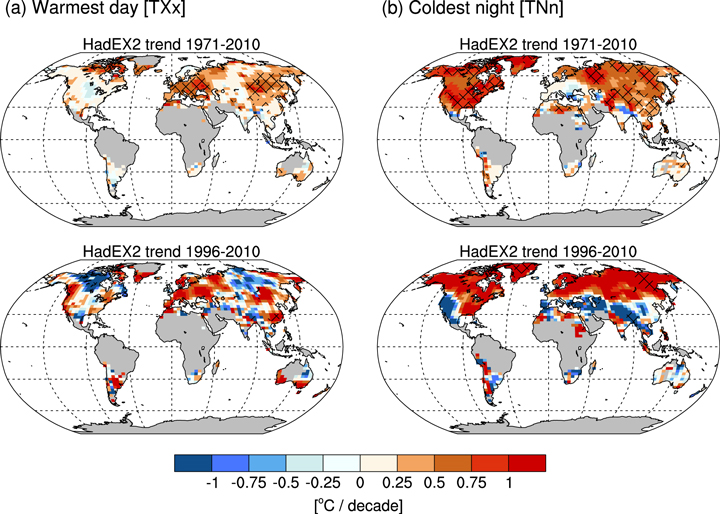
Figure 1. Trends in the (a) warmest day (TXx, annual maximum of Tmax) and (b) coldest night (TNn, annual minimum of Tmin) for the last 40 years (1971–2010) (upper panel) and for the recent 15 years (1996–2010) of the HadEX2 dataset. Hatching indicates where trends are significantly different from zero to the 95% confidence level (p < = 0.05) (see text for details). Grid boxes for which data was available for at least 38 years out of the 40 year period (1971–2010) are shown in color.
Download figure:
Standard image High-resolution imageThe coldest night in a year (TNn), usually occurring in winter, show stronger significant positive trends than TXx over the last 40 years in large parts of the Northern Hemisphere, except in Southern and Central Europe (figure 1(b)). In the recent 15 years, the northern latitudes show strong warming trends (∼1 °C per decade), but a coherent zonal band of cooling trends (although again not statistically significant) emerges in the mid-latitudes including western North America and Southern Europe stretching all the way to East Asia. Cooling trends are also prevalent in some areas with sufficient observational data in the Southern Hemisphere (i.e., Southern South America, South Africa and parts of Australia). Note that even if we see a cooling trend regionally (as in figure 1), globally averaged TNn and TXx in the recent 15 years remain on average warmer as observed in the preceding 25 years (i.e., 1971–1995) (see supplementary figure S1). Thus, short-term regional cooling trends do not undermine the global long-term warming trend.
Looking at the median of trends estimated from the ensemble of CMIP5 model simulations in figure 2, we see that significant positive trends in both TXx and TNn dominate across the globe during the past 40 years. In the recent 15 years, some small areas with no or slight cooling trend become apparent; however, these patterns are much less pronounced and not as coherent as in HadEX2. More notable is the similarity between trend patterns over the past 40 years compared to the past 15 years in the model simulations. The ensemble median pattern indicates the dominance of positive trends as found in the bulk of model simulations and masks cooling trends that are apparent in some individual ensemble members. For instance, globally averaged cooling trends in TNn during 1996–2010 occur in individual ensemble realizations of four CMIP5 models (see online supplementary table S1). The observed spatial TNn trend pattern is reasonably reproduced by two of these models (CMCC-CMS and CSIRO-Mk3-6-0, see supplementary figure S2). All models, except MRI-CGCM3, simulated a globally averaged warming trend in TXx in the recent 15 years.

Figure 2. Same as figure 1, but for the CMIP5 ensemble median of TXx and TNn time series based on 27 models with individual models having multiple ensemble members (see online supplementary table S1). Note, only grid boxes for which HadEX2 data was available for at least 38 years out of the 40 year period (1971–2010) are shown in color.
Download figure:
Standard image High-resolution imageFrom this analysis, regional and seasonal features in TNn and TXx become apparent that are not seen when studying globally averaged Tmean alone. Spatial and seasonal features in Tmean have been discussed in Kosaka and Xie et al (2013) and Cohen et al (2012), but those patterns cannot be directly compared to the TXx and TNn patterns shown here because different mechanisms are involved in generating extreme minimum night-time or maximum day-time temperature conditions compared to Tmean (Seneviratne et al 2014). We should therefore not expect that they could be inferred from a simple first-order shift in the temperature distribution.
3.2. Zonal trend patterns
An interesting feature in figure 1(b) is the zonal structure of the cooling trends in observed cold extremes in the last 15 years. We investigate this in more detail by looking at zonally averaged time series of 15-year running trends in HadEX2 and the models for the period 1971–2010. We distinguish between zonal bands including the high latitudes in the Northern Hemisphere (45 °N–90 °N) and the mid-latitudes in both Hemispheres (20 °S–45 °S and 20 °N–45 °N). We exclude the low latitudes (i.e., 20 °S–20 °N) due to sparse observational data coverage.
As we have seen, individual trend estimates based on short (i.e., 15-year) records are highly uncertain. A technique such as that of Fyfe et al (2013) can nevertheless be used to determine whether a collection of model simulated trends as obtained from an ensemble of climate simulations is consistent with an observed trend. Thus, our objective in this section is to investigate question (b) as to whether model simulated trends in temperature extremes are consistent with observed trends.
Running 15-year trends in globally averaged TXx and TNn from HadEX2 lie within the 90% range of model trends (i.e., 5–95% of the models in the following) for both TXx and TNn as can be seen in figure 3. For TXx, the ensemble median and range of the running 15-year model trends follows the evolution of observed 15-year running trends in HadEX2 particularly at the global scale, and also for the zonal averaged latitudinal bands, except in the higher northern latitudes (45 °N–90 °N). In the latter region, the observed trend falls outside the model range in the mid-1980's, where also the null hypothesis (i.e., observed and simulated trends are equal) is rejected for both assumptions discussed in Fyfe et al (2013). This single departure is, however, within the expected rejection rate of a statistical test that has a nominal significance level of 10%. It appears that rejections are actually very rare, suggesting that intermodel differences are probably larger than internal variability (i.e., evidence of a discrepancy between observed and simulated trends has to be strong to reject).

Figure 3. Time series of 15-year running trends for the coldest night (TNn, left panels) and warmest day (TXx, right panels) for the CMIP5 multi-model ensemble, where trends are derived from zonal averages of local TXx and TNn anomalies. The solid black line indicates the multi-model median and the shading the 5–95% model range (see online supplementary table S1 for a list of all models and their ensemble members). The red line indicates the 15-year running trend for the corresponding HadEX2 indices. Blue circles indicate where the null hypothesis is rejected (i.e., observed and simulated trends are equal) for both assumptions according to Fyfe et al 2013 (see text for details).
Download figure:
Standard image High-resolution imageFor TNn, the temporal evolution of the HadEX2 running 15-year trends is more variable than the corresponding evolution of TXx in HadEX2. Observed global features in TNn, such as the larger trends in the 1980s and comparably smaller trends in the recent 15 years, are neither found in the model ensemble median nor range. This feature manifests itself in the mid-latitudes, and particularly in the Northern Hemisphere mid-latitudes (20 °N–45 °N), where observed trends fall outside the model range in a sequence of years between the late 1990s and early 2000s. This again is supported by the rejection of the null hypothesis of the applied test statistic. Similar results can also be found when considering 20-year running trends (see supplementary figure S3). The steep increasing trend in observed TNn in the higher northern latitudes (45 °N–90 °N) is embedded in the comparably wide model range for this zonal band, but is not reproduced in its full extend by the ensemble median.
3.3. Regional trend patterns
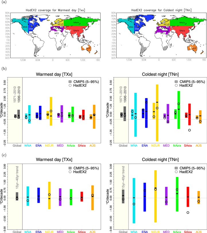
To pin down regional patterns of recent observed and simulated trends, we compare trends in globally and regional averaged TXx and TNn for the two time periods. We choose seven continental-scale regions (see figure 4(a)) according to the HadEX2 data coverage as well as climatological features of observed trend patterns, as discussed in section 3.1. Note, that the trends in globally averaged TXx and TNn do not represent the sum of the averages over the seven regions as grid-boxes in South America and South Africa (gray shading in figure 4(a)) are not included in any of the defined regions.
Figure 4. (a) Maps for all available grid boxes with sufficient HadEX2 coverage for the warmest day (TXx, left panel) and the coldest night (TNn, right panel) for the globe (i.e. GLOBAL, 60S-90N, including colored regions and gray areas) and for the seven regions indicated in color in the maps. (b) Trends for two periods (1971–2010 and 1996–2010) in spatially averaged TXx (left) and TNn (right) for the globe and seven regions for HadEX2 (black circle) and the CMIP5 model simulations (see online supplementary table S1), where the bars indicate the 5–95% ensemble range and the ensemble median is marked as black line. (c) Differences in trends over the recent 15 years (1971–2010) minus the longer 40 year period (1996–2010) for global and regional averages of TXx (left) and TNn (right).
Download figure:
Standard image High-resolution image
As can be seen in figure 4(b), the observed trends in globally averaged TNn and TXx fall within the 5–95% model range. Compared to the test results (i.e., using the method of Fyfe et al 2013) presented in the previous section 3.2., the model range represents a rather conservative estimate of whether the observed trends are consistent with the simulated trends. Thus, in the following, we consider only the model range as the basis for our comparison of regional trends from models and observations. Note that the global results shown in figure 4(b) for the 1996–2010 period are identical to the last time point shown in the panels of the upper row of figure 3. Note also that the model spread is substantially wider when a shorter period is considered (i.e., 1971–2010 versus 1996–2010), as is expected due to the greater uncertainty in trend estimates from the shorter records. In general, the observed trends of globally averaged TNn and TXx are comparable between the recent 15-year and the longer 40-year period with the differences between the trends of the two periods centering around zero (figure 4(c)).
Recent detection and attribution studies by Zwiers et al (2011) and Christidis et al (2011) as well as a detection study by Fischer and Knutti (2014) argue that models generally underestimate observed trends in globally averaged TNn and some models overestimate observed trends in globally averaged TXx. If we repeat our analyses using the set of CMIP5 models and ensemble members as in online supplementary table S1 for similar periods as considered in these studies (e.g., 1960–2000, 1971–2000, 1960–2010), we generally confirm these results (see supplementary figure S4). This comparison, however, reveals that there is some sensitivity to the time period chosen for the comparison of simulated and observed trends, particularly when limiting the model information to one number (i.e., the ensemble median or mean).
We look now at regional scales and as at the global scale we find again that the trends in simulated TXx are generally in agreement with the observed trends (figure 4(b), left), with particularly close agreement in Australia (AUS) and North Asia (NAsia) for both periods. Differences between the longer and shorter period generally center on zero (figure 4(c), left) for both observed and simulated trends in all regions, which indicates comparable trends between these two periods.
Larger regional discrepancies are found between simulated and observed trends in TNn (figure 4(b), right). The observations show moderate to pronounced negative trends in the recent 15 years in several regions (particularly in Southern Asia (SAsia)), whereas the majority of models simulate a positive trend. Only one model (i.e., CCSM4) simulated a negative trend as large as the observed in SAsia (see also supplementary figure S2(b), (c)). For this region, the observed difference in TNn trends between the shorter and longer period falls outside the 5–95% model range of differences (figure 4(c), right). This indicates a discrepancy between the observed and simulated trends for the recent 15 years as reflected also in the statistically significant departure of observed running trends from the range of simulated trends in the northern mid-latitudes as shown in figure 3.
For the other regions, observed trends in TNn fall within the range of simulated trends (figure 4(b)). Differences between the two periods deviate further from zero than for trends in TXx (figure 4(c)), indicated by the larger model spread, but still center around zero. Slight cooling trends in HadEX2 in the recent 15 years can be found in the Mediterranean region (MED) and AUS, which however fall within the model range. In the other regions, located primarily in the mid-to-high northern latitudes (i.e., Eastern North America (ENA), Northern Europe (NEUR) and Northern Asia (NAsia)), the observations show an increased warming trend for TNn in the recent 15 years compared to the longer period, which is also reflected in the ensemble median. In general, it becomes apparent that the warming trend in the recent 15 years is somewhat more pronounced in cold extremes (i.e., TNn) in high northern latitudes, and exceeds the warming observed in the hot extremes (i.e., TXx).
4. Summary and conclusion
The evaluation of differences between trends requires consideration of all sources of variability that affect the trend estimates. As has been demonstrated many times previously, uncertainty depends upon both the length of the period that is considered, and the domain that is used to spatially average climate quantities prior to trend estimation. Both record length and spatial domain affect sampling uncertainty that arises from internal variability in the climate system, with larger relative uncertainty being associated with shorter records and smaller regions, and internally generated natural variability dominating short-term simulations (Hawkins and Sutton 2009, Santer et al 2011). The methods used in this paper account for those effects to the extent that internal variability is well simulated in climate models, which constitutes a research question in itself.
We analyzed observed and model-simulated trends in annual temperature extremes for the past 40 years (1971–2010) in comparison to the recent 15 years (1996–2010) using climate extreme indices from the HadEX2 observational dataset and a large set of CMIP5 models. Simulated trends over the two periods are generally comparable to observed trends for absolute temperature extremes (i.e., coldest night (TNn) and warmest day (TXx) of the year) on a global scale. The observed trends in hot extremes (i.e., TXx) are well represented in climate simulations, showing warming trends similar to those seen in the observations in both periods. Observed warming trends in cold extremes (TNn) are less well represented in climate simulations, but simulated trends are nevertheless consistent with observed trends globally and in many regions. The largest discrepancy between observed and simulated trends in cold extremes is found in the Northern mid-latitudes (20 °N–45 °N), where observations indicate a coherent zonal band of decreasing trends over the recent 15 years. This might be connected to the recent hiatus in the warming of global Tmean, which has been characterized mainly as a winter phenomenon (e.g., Kosaka and Xie 2013, Cohen et al 2012). Only a few individual model realizations simulate a cooling trend in TNn.
Our findings are consistent with the suggestion that the recent 15-year period largely represents a highly unusual (extreme) realization of climate as part of internal variability (e.g., Meehl et al 2013, Kosaka and Xie 2013, England et al 2014). Other recent studies (Fyfe et al 2013, Fyfe and Gillett 2014) argue that internal climate variability is unlikely to be the only explanation for the discrepancy seen between model and observed trends and that some external forcing components not fully represented in current climate models could have contributed to the local cooling trends in cold extremes. While precisely identifying the mechanisms behind the observed regional cooling patterns in extreme cold temperatures lies beyond the scope of this paper, the results presented here provide relevant details to complete the overall picture of recent temperature changes beyond globally averaged Tmean.
We conclude that while there appears to be a discrepancy in global Tmean trends between observations and simulations over the hiatus period (e.g., Fyfe et al 2013), that discrepancy does not generally extend to temperature extremes, with the exception of a recent cooling in Northern mid-latitude TNn that is particularly apparent regionally in South Asia. In general, temperature extremes continue to increase in most regions of the world consistent with the long-term projections under global warming scenarios (e.g., Seneviratne et al 2012, Sillmann et al 2013b).
Acknowledgements
We acknowledge the World Climate Research Programme's Working Group on Coupled Modelling, which is responsible for CMIP, and we thank the climate modeling groups for producing and making available their model output. For CMIP the US Department of Energy's Program for Climate Model Diagnosis and Intercomparison provides coordinating support and led development of software infrastructure in partnership with the Global Organization for Earth System Science Portals. J S was supported by the German Research Foundation (grant Si 1659/1-1) as well as through the AERO-CLO-WV and NAPEX project, both funded by the Norwegian Research Council. M G D received funding through the Australian Research Council grants LP100200690 and CE110001028.