
Abstract
Very large-fires (VLFs) have widespread impacts on ecosystems, air quality, fire suppression resources, and in many regions account for a majority of total area burned. Empirical generalized linear models of the largest fires (>5000 ha) across the contiguous United States (US) were developed at ∼60 km spatial and weekly temporal resolutions using solely atmospheric predictors. Climate−fire relationships on interannual timescales were evident, with wetter conditions than normal in the previous growing season enhancing VLFs probability in rangeland systems and with concurrent long-term drought enhancing VLFs probability in forested systems. Information at sub-seasonal timescales further refined these relationships, with short-term fire weather being a significant predictor in rangelands and fire danger indices linked to dead fuel moisture being a significant predictor in forested lands. Models demonstrated agreement in capturing the observed spatial and temporal variability including the interannual variability of VLF occurrences within most ecoregions. Furthermore the model captured the observed increase in VLF occurrences across parts of the southwestern and southeastern US from 1984 to 2010 suggesting that, irrespective of changes in fuels and land management, climatic factors have become more favorable for VLF occurrence over the past three decades in some regions. Our modeling framework provides a basis for simulations of future VLF occurrences from climate projections.
Export citation and abstract BibTeX RIS

Content from this work may be used under the terms of the Creative Commons Attribution 3.0 licence. Any further distribution of this work must maintain attribution to the author(s) and the title of the work, journal citation and DOI.
Corrections were made to this article on 9 December 2014. The affiliations were corrected, adding the fourth author.
1. Introduction
Large wildfires that compose a small percent of total fires but often a majority of burned area (Strauss et al 1989, Tedim et al 2013) have shown a marked increase across parts of the globe including the western United States (US) in recent decades (Dennison et al 2014). These large wildfires have direct societal and ecological impacts (Gill and Allan 2008, Keane et al 2008), widespread impacts to regional air quality and human health (e.g., Clinton et al 2006) and global climate feedbacks (e.g., Liu et al 2010). The spatial extent and resistance to control often make such large wildfires among the most dangerous and costly wildfires (Williams 2012).
In the US, large wildfires are inherent to certain fire regimes and may have been more pervasive in some regions prior to human settlement (e.g., Stephens et al 2007). Fundamental to the development of large-fires (LFs) are widespread and contiguous fuels, ignitions, and environmental conditions that promote fuel availability and spread (Swetnam and Betancourt 1990, Hawbaker et al 2013). The accumulation of fuel loads due to land management practices (e.g., Miller et al 2009) and invasive annual grasses across the semi-arid western US (e.g., Abatzoglou and Kolden 2011b, Balch et al 2013) are hypothesized to have created a more favorable environment for LFs in recent decades. However, the receptiveness of fuel to fire and fire spread are strongly driven by both weather and climate variability. In particular, they respond to antecedent climatic factors that enable landscape-level fuel availability (Dennison et al 2014), as well as to concurrent dead and live fuel moistures (Dennison and Moritz 2009) and favorable meteorological conditions that promote fire spread and impede suppression efforts (e.g., Abatzoglou and Kolden 2011a). It is not presently resolved to what degree observed changes in climate have contributed to the increase in LFs relative to other human activities (e.g., Westerling et al 2006, Marlon et al 2012, Pausas and Keeley 2014). As fire potential is projected to increase for parts of the US under climate change scenarios (Spracklen et al 2009, Liu et al 2012, Luo et al 2013), efforts to better understand empirical and processed-based links between climate and fire have received increasing interest.
Most climate−fire studies have analyzed interannual relationships using temporal and geographic aggregations of burned area and climate variables (e.g., Skinner et al 1999, Westerling and Swetnam 2003, Littell et al 2009, Abatzoglou and Kolden 2013) and have extended these to empirical modeling efforts (e.g., Yue et al 2013, Migliavacca et al 2013). Although some statistical models have been designed to forecast daily fire potential using fire danger indices and ignitions (Preisler et al 2009), the complex empirical relationships linking atmospheric variability and the development of LFs is not fully resolved across different geographic regions or fire regimes. Recent work by Stavros et al (2014a) and Barbero et al (2014) demonstrate significant differences between climatic conditions associated with the very largest fires and other large fires, in the western and eastern US, respectively. However, these studies were based on regional-scale fire aggregations (∼500 km) and did not account for regional heterogeneity that are needed for operational or research purposes.
This study extends previous work by developing Generalized Linear Models (GLM) to simulate probabilities of very large-fire (VLF) (>5000 ha) occurrences across the US at a 60 km spatial and weekly temporal resolution using strictly atmospheric variables. Specifically, we identify the most important weather and climate predictors of VLF occurrences across ecoregions. Estimates from GLM were evaluated by comparing model predictions to observed VLFs across both space and time. Finally, we compare observed and modeled linear trends from 1984 to 2010 to better resolve the degree to which atmospheric conditions alone have potentially enabled changes in VLFs. This modeling framework aims to provide seasonal-to-short term outlooks for operational fire management as well as guidance on how climatic conditions may alter the occurrence of VLFs under future climates.
2. Datasets and methods
2.1. Fire and climate data
The myriad of fire regimes across the contiguous US (Morton et al 2013) is problematic for generalizing climate−fire relationships. Most prior analysis and modeling has been conducted using aggregated fire and climate data over broad geographic and temporal scales. Modeling efforts at finer spatial scales have been conducted to better link environmental factors such as vegetation, topography, climate and anthropogenic factors (Parisien et al 2012, Hawbaker et al 2013); however, such models are often time invariant or may not be designed to model rare events such as VLFs.
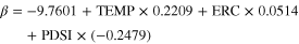
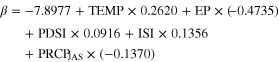
We provide a compromise of spatiotemporal scales in this study by examining relationships between VLFs and climate factors at a 60 km spatial and weekly temporal resolution for Omernik level II ecoregions (Omernik 1987). Ecoregions broadly reflect climate and vegetation zones with similar climate−fire responses (e.g., Littell et al 2009, Malamud et al 2005) while providing a suitable number of VLFs required to build stable and meaningful models. However, heterogeneity in climate and fire regimes exists at sub-ecoregion scales thus prompting the need to refine the spatial scale of modeling. We model intra-ecoregion variability at tractable scales that reflect the spatial extent of the variability of top-down controls of fires, by spatially aggregating ecoregion to ∼60 km resolution using the most common ecoregion within each voxel (figure 1(a)). We excluded ecoregions that experienced fewer than five VLFs from 1984 to 2010 as well as all ∼60 km pixels where a majority of land cover from a 1 km fuel model map (Burgan et al 1998) was non-burnable defined by the presence of agriculture and barren land cover types.
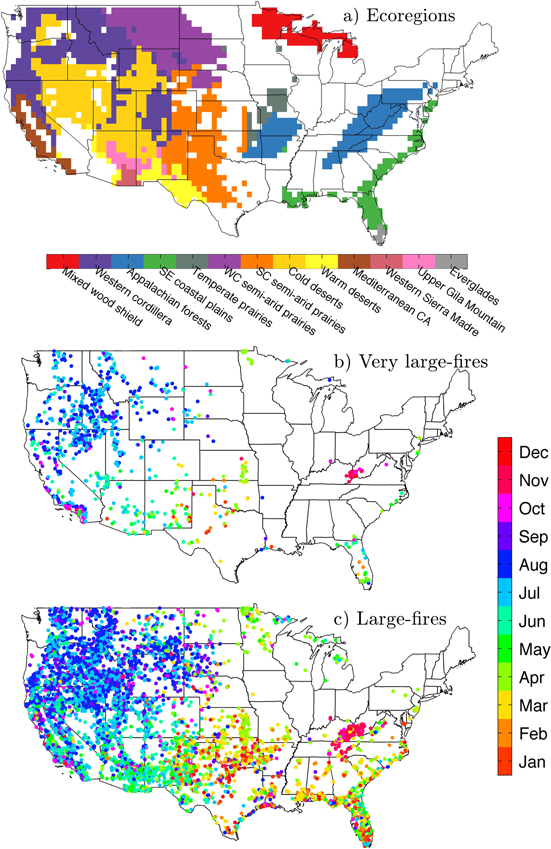
Figure 1. (a) Aggregated ecoregions at ∼60 km. We excluded all pixels where a majority of land cover from 1 km fuel model map (Burgan et al 1998) was non-burnable defined by the presence of agriculture and barren land cover types. Spatiotemporal occurrences of (b) VLF (fire whose size >90th) and (c) LF (fire whose size <90th) (1984–2010). Models are built from VLF occurrences and evaluated from LF occurrences.
Download figure:
Standard image High-resolution imageThe Monitoring Trends in Burn Severity (MTBS) database was used to acquire fire location, fire discovery date and burned area for LFs over the contiguous US from 1984 to 2010. We excluded fires smaller than 404 ha and further eliminated 'unburned to low' burned area for each fire as classified by MTBS to more accurately portray the true area burned (Kolden et al 2012). While the definition of VLFs is subjective and likely geographically dependent, we define VLFs as fires whose size exceeds the 90th percentile (5073 ha) of MTBS fires greater than 404 ha (n = 927) (figure 1(b)) and LF as fires whose size was below the 90th percentile but greater than 404 ha (n = 8343)(figure 1(c)). Both VLF and LF were aggregated to ∼60 km grid and six-day time increment (hereafter we will use the term 'week' for simplicity) yielding a time series of 1647 weeks from 1984 to 2010 coded as 1 if at least one VLF was discovered within that week, and 0 otherwise, for each voxel. Modeling at the weekly timescale has the advantage of capturing intra-seasonal variability otherwise masked in longer timescales and important for VLF (Barbero et al 2014). However, we acknowledge that this temporal aggregation may mask intra-weekly spread events, when weather conditions are conducive to fire spread (Podur and Wotton 2011, Wang et al 2014).
We considered a set of predictor variables intended to capture different timescales of variability through which the atmosphere can influence VLF occurrences from synoptic to sub-seasonal to interannual scales (table (S1)). We selected potential predictors used in prior climate−fire studies to limit model complexity, although this list is by no means exhaustive. Daily surface meteorological variables at a ∼4 km spatial resolution were obtained from Abatzoglou (2013). We first considered several concurrent variables averaged at the weekly scale coinciding with the VLF database. These included mean temperature and relative humidity (average of daily maximum and minimum), as well as four fire danger indices: Energy Release Component (ERC) and Burning Index (BI) from the National Fire Danger Rating System (Deeming et al 1977), using fuel model G, Initial Spread Index (ISI) from the Canadian Forest Fire Danger Rating System (Van Wagner 1987) and Fosberg Fire Weather Index (FFWI, Fosberg 1978). Two concurrent drought indices were used: (i) the 30-day Effective Precipitation (EP) index (Byun and Wilhite 1999) that sums rainfall over the previous 30-days with a daily weight decreasing in a non-linear fashion that has been shown to be a proxy for surface soil moisture, and landscape flammability (Barbero et al 2011), and (ii) the Palmer Drought Severity Index (PDSI) given its widespread usage in climate−fire studies (e.g., Westerling and Swetnam 2003). We also considered PDSI from the year prior averaged over the growing season May−September (hereafter  ), as it has been linked to changes in biomass availability in fuel-limited fire regimes.
In addition to temporally varying predictors, we considered a set of time invariant variables to potentially account for heterogeneity in vegetation at sub-ecoregion scales as they pertain to wildfire potential. Rather than using bottom-up controls (e.g., actual distribution of vegetation), we considered climatological normals of actual evapotranspiration and Climatic Water Deficit (CWD) following Dobrowski et al (2013) as proxies of potential productivity and moisture stress (Parks et al 2014). Balch et al (2013) showed that fire activity throughout much of the Cold Deserts ecoregion was facilitated by the presence of an invasive annual grass (Bromus tectorum). We thus considered the fraction of total annual precipitation in July−September ( ) as a potential predictor given that Bradley (2009) found that it constrained the geographic distribution of Bromus tectorum. Note that these predictors are reasoned to model conditions conducive to VLF and not the exact location of VLF, since we did not include ignition sources.
2.2. Modeling approach
Models describing rare binary events are, by definition, designed from small samples, are often imbalanced and over-fitted and consequently may not be robust. Therefore, additional procedures are required in the modeling of rare events to ensure stable and reproducible models (Austin and Tu 2004, Keating and Cherry 2004). We employed resampling methods in model development and cross-validation to assess model robustness.
We used GLM with a stepwise regression given their ability to model binary data (Andrews et al 2003, Stavros et al 2014a). Models were developed for each ecoregion acknowledging regional differences in the biophysical drivers manifest through vegetation and climate, as well as human factors (e.g., ignitions and suppression). We applied a case-control design (Keating and Cherry 2004) that uses all VLF weeks and resampling with replacement of non-VLF weeks drawn from the distribution of all voxels across time for each ecoregion (see supplementary materials for further details, available at stacks.iop.org/ERL/9/124009/mmedia).
The continuous probabilities given by GLM were used to analyze VLF probability as they have the advantage of being able to quantify the uncertainty associated with the simulation in a given voxel. We compared modeled VLF probabilities (P) with observed VLF weeks at the voxel level to assess model credibility in both space and time. The latter was examined using composite analysis of P both ten weeks prior to and ten weeks following observed VLF weeks. The analysis was repeated using LF weeks, as an additional cross-validation analysis. Seasonal and interannual variability was assessed by aggregating data to ecoregions and using Spearman rank correlations between P and observed VLF (note that p aggregated over timescales and/or ecoregions refers to the number of VLF weeks). Linear least-squares trends in the total number of VLF-weeks in observations and simulated P were analyzed from 1984 to 2010 for each ecoregion and are referred to as statistically significant when the 95% confidence interval excludes no change in the sign of the trend. Linear trends in mean annual P were analyzed as well. We emphasize the use of continuous P in our analyses given the challenges in converting these values to binaries. However, we acknowledge that the use of continuous P for rare events tends to minimize variance thereby underestimating the probability of highly likely events and vice-versa, resulting in reduced interannual variability and trends. We complement continuous P by converting P into binaries ( ) by using a threshold that equals the ratio of number of VLF weeks to total weeks for all voxels within each ecoregion.
3. Results
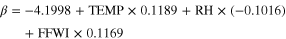
Except in the Cold Deserts, three or fewer predictors were selected in GLM models for each ecoregion, with most ecoregions relying on two or fewer variables (table 1). Short-term variability represented though ISI, BI, FFWI, temperature or relative humidity was a significant predictor of VLF occurrences in ten ecoregions while sub-seasonal variability realized through ERC or EP was a significant predictor in six ecoregions. Concomitant longer-term drought represented by PDSI was an important contributor of VLF in flammability-limited ecoregions such as Western Cordillera and Appalachian forests, while anomalous wet conditions realized through PDSI in the year prior to or concurrent with was a significant predictor in a couple fuel-limited ecoregions. Annual mean CWD and  were selected as predictors in Mixed Wood Shield and Cold Deserts, respectively, largely reflecting spatial variations in VLF within these ecoregions. Our results suggest that these models are robust given the large commonality across bootstrapped samples and exhibited high skill across ecoregions (table 1), although other combinations of predictors are possible.
Table 1. Equations describing weekly VLF probabilities at 60 km for each ecoregion.
| Ecoregions | #VLF weeks |

|

|
RF (%) |
|---|---|---|---|---|
| Mixed Wood Shield | 8 |

|
0.95 | 49 |
| Western Cordillera | 208 |
|
0.95 | 20 |
| Appalachian forests | 20 |

|
0.91 | 96 |
| Southeast Coastal Plain | 27 |

|
0.89 | 99 |
| Temperate Prairies | 5 |

|
0.95 | 85 |
| WC Semi-arid Prairies | 34 |

|
0.96 | 96 |
| SC Semi-arid Prairies | 58 |

|
0.84 | 21 |
| Cold Deserts | 276 |
|
0.95 | 82 |
| Warm Deserts | 23 |

|
0.90 | 79 |
| Mediterranean California | 70 |
|
0.90 | 23 |
| W. Sierra Madre Piedmont | 18 |

|
0.95 | 86 |
| Upper Gila mountain | 25 |

|
0.87 | 92 |
| Everglades | 8 |

|
0.84 | 85 |
Note: Predictors were selected with stepwise regression from 1000 Monte-Carlo samples including all VLF weeks and 50 000 random non-VLF weeks. We used the most frequent equation among the 50 000 simulations. The second column gives the number of VLF weeks observed in each ecoregion. The third column gives  parameters (intercept and coefficients) averaged over the 50 000 cross-validated Monte-Carlo simulations.
  is the is the fraction of non-VLF weeks randomly sampled compared to the number of non-VLF weeks in the population. The fourth column indicates the mean area under the curve between simulated very large-fire probabilities and observations according to the cross-validated model (see supplementary materials for further information). The fifth column gives the relative frequency (RF) of the equation, i.e. the percent of simulations in which there was agreement.
The mean number of VLF weeks expected was highest across the western US between May and September, consistent with the observed distribution of VLF and their timing (figure 2). The seasonality of P aggregated to the ecoregion scale showed strong agreement with observations (table 2), except for the Appalachian forests. Additional heterogeneity in seasonal variability was simulated within each ecoregion with the seasonal timing of peak VLF probability (figure 2), mainly agreeing with the timing of observed VLF (figure 1(b)). For example, P for the Mediterranean California ecoregion peaks in late summer in the northern and interior portions of the region, while peaking in autumn in the coastal mountains and plains of southwestern California coincident with Santa Ana driven wildfires.
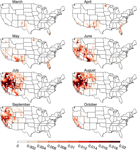
Figure 2. (a) Mean monthly number of VLF expected averaged over the 1984–2010 period from climate−fire model outputs.
Download figure:
Standard image High-resolution imageTable 2.
Spearman rank correlations between VLF observed  and the number of VLFs expected from continuous probabilities (
 ) and binary probabilities
  summed over each month (1st and 2nd columns) and over each year (3rd and 4th columns).
| Ecoregions | Monthly scale 
|
Monthly scale 
|
Interannual 
|
Interannual 
|
Trend in 
|
Trend in 
|
Trend in 
|
|---|---|---|---|---|---|---|---|
| Mixed Wood Shield | 0.57+ | 0.77+ | 0.52+ | 0.67+ | −0.2 | 0.0 | −0.3 |
| Western Cordillera | 0.96+ | 0.87+ | 0.73+ | 0.62+ | 4.1* | 1.9 | 4.6 |
| Appalachian forests | 0.27 | 0.23 | 0.30 | 0.34 | −0.6 | 0.0 | −0.7 |
| Southeast Coastal Plain | 0.87+ | 0.33 | 0.55+ | 0.49+ | 0.3 | 0.4* | 0.3 |
| Temperate Prairies | 0.60+ | 0.74+ | 0.44+ | 0.76+ | 0.1 | 0.0 | 0.0 |
| WC Semi-Arid Prairies | 0.85+ | 0.80+ | 0.68+ | 0.71+ | 0.5 | 0.0 | −0.2 |
| SC Semi-Arid Prairies | 0.86+ | 0.90+ | 0.73+ | 0.77+ | 2.0* | 0.6* | 2.5 |
| Cold Deserts | 0.87+ | 0.94+ | 0.57+ | 0.43+ | 2.4 | 1.2 | 7.2* |
| Warm Deserts | 0.91+ | 0.75+ | 0.57+ | 0.64+ | 1.2* | 0.3* | 0.4 |
| Mediterranean California | 0.90+ | 0.85+ | 0.49+ | 0.58+ | 1.0* | 1.1* | 3.5* |
| Sierra Madre Piedmont | 0.87+ | 0.92+ | 0.55+ | 0.67+ | 0.3 | −0.1 | 0.3 |
| Upper Gila Mountain | 0.85+ | 0.82+ | 0.44+ | 0.50+ | 0.5* | 0.3* | 0.9 |
| Everglades | 0.47 | 0.55+ | 0.61+ | 0.78+ | 0.5* | 0.1* | 0.5* |
Note: The symbol + indicates significant correlation at the 95% confidence level. Linear trends in  (expressed as number of VLF per decade),
  and
and  are shown in columns 5, 6 and 7 respectively. The symbol * indicates that the 95% confidence interval excludes no change in the sign of the trend.
We provide examples of modeled VLF probabilities during the discovery week of four notable VLF fires (figure (S2)): Zaca fire in California during July 2007, the Bugaboo fire on the Georgia/Florida border during April 2007, the Rodeo-Chediski fire in Arizona during June 2002 and the Day fire in California during September 2006. For all cases, regional VLF probabilities were elevated and locally almost 300% above normal compared to the mean seasonal cycle. As our models do not include ignition sources, or other bottom-up variables (e.g., topography, population) and incorporate predictors with strong spatial autocorrelation, they should not be expected to capture the exact location of the fire, but rather local-to-regional enhancements in P. Figure 3 shows the composite of P anomalies georeferenced relative to centroids of observed VLF. The strong signal decaying radially from the fire centroid suggests the model captured local-to-regional enhancement in P, with signal attenuation consistent with the spatial autocorrelation of most predictor variables. A temporal composite analysis for voxels reporting VLF-weeks shows peak P during the week of fire discovery (200% above climatology) with enhanced probability in the weeks prior to and following as expected with the serial correlation of many of the predictors used (figure 3(b)). Composite analysis for observed LF weeks showed above normal P, albeit weaker than for VLF weeks (figure 3(b)).
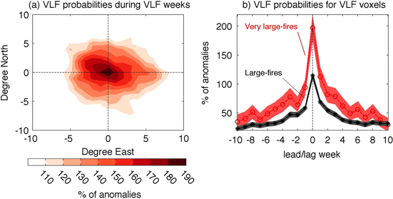
Figure 3. (a) Mean VLF probabilities (expressed in percent of anomalies compared to the mean local seasonal cycle) at the US scale from climate−fire models during VLF weeks. The probabilities have been relocated relative to VLF locations (coordinates: 0, 0) such that the center of the map corresponds to the location of each VLF. (b) Composites of probabilities in VLF voxel relative to the discovery week of VLF. The red (black) curve indicates the mean probabilities simulated before and after VLF (LF) weeks. The 95% confidence intervals of the composite means are computed using 1000 bootstrapped datasets. The envelope of confidence indicates the 2.5 and 97.5 percentile of the composite means obtained from the bootstrapped datasets.
Download figure:
Standard image High-resolution imageInterannual variability in P aggregated to ecoregions showed reasonable agreement with observations, with correlations r > 0.5 in most ecoregions (table 2). While aggregating such statistics within an ecoregion may enhance low frequency variations in climate anomalies typically present in longer-term and seasonal predictors (e.g., PDSI, ERC), the same may not hold for all regions. For instance, weaker correlation in the Cold Deserts, albeit significant, is likely a product of the extensive longitudinal and latitudinal extent of the ecoregion that straddles a latitudinal dipole in interannual precipitation variability across the western US that dilutes low-frequency variability across the aggregated ecoregion.
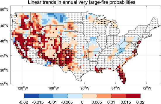
A positive trend in mean annual P was found for 1984–2010 across much of the western half of the US, but also across some regions in the east, including the Southeast coastline and Florida (figure 4). Likewise, an increase in VLF occurrence has been documented in most southern ecoregions (table 2). Some ecoregions such as the Cold Deserts and Western Cordillera spanned a significant latitudinal extent that may mask trends apparent on a regional basis. Simulated trends from continuous probabilities were weaker but statistically more robust than trends from binary probabilities.
Figure 4. Trends in annual number of VLFs expected from simulated probabilities for the 27-year period from 1984 to 2010. Dots indicate trends for which 95% confidence interval excludes no change in the sign of the trends. Gray dots indicate pixels defined as unburnable or pixels associated with ecoregions that did not record more than five VLF over the historical period.
Download figure:
Standard image High-resolution image
4. Discussion
Measures to develop statistical models through resampling techniques improve model stability and overcome some limitations of modeling relatively rare events (i.e., large imbalance between events and non-events). Although the form of the equations relies on the choice of inputs variables used in stepwise regression (e.g., table 1), resampling schemes helps select robust predictors. The resultant models make intuitive sense and concur with established interannual climate−fire relationships (e.g., Littell et al 2009) while also accounting for sub-seasonal timescales that have been documented to be favorable for LFs growth (e.g., Abatzoglou and Kolden 2011a). However, further efforts may better account for intra-weekly spread events driven by shorter-term weather variability (Wang et al 2014).
Our models show that VLF are often enabled by a combination of atmospheric conditions operating on synoptic to interannual timescales. Synoptic variability has been shown to be a significant driver of VLF occurrences, especially in non-forested ecoregions where rapid fire spread is favored by extreme fire-weather, as for example during Santa Ana wind driven fires in Southern California (Keeley et al 2004, Moritz et al 2010). However, short timescales of synoptic variability may be insufficient to carry VLF in forested ecoregions such as Western Cordillera where fires typically grow over a longer time period. Instead, sub-seasonal drought viewed through ERC was a key predictor of VLF in these flammability-limited ecoregions in agreement with previous findings (Riley et al 2013, Barbero et al 2014, Stavros et al 2014a). Concurrent long-term drought described by PDSI was a complimentary predictor in the Appalachian forests and Western Cordillera. These results concur with previous climate−fire linkages (Westerling and Swetnam 2003, Littell et al 2009) and the longer time period under moisture stress required to increase landscape flammability in ecosystems dominated by large-diameter trees. Antecedent moisture availabilities ( ) was a significant predictor in two fuel-limited ecoregions reinforcing heighten fire activity that corresponds to increased fuel biomass and connectivity a year following pluvial conditions (e.g., Westerling and Swetnam 2003, Littell et al 2009). By contrast, VLF probabilities increased with concurrent positive PDSI in Warm and Cold Deserts corresponding to the rapid growth and desiccation of fine fuels in arid regions (Crimmins and Comrie 2004). Two time-invariant predictors were also selected and improved the spatial accuracy of the model. Increased CWD increased probabilities in Mixed Wood Shield ecoregion, consistent with the findings of Parks et al (2014) that drier regions are more susceptible to moisture stress. Finally, the fraction of summer precipitation in July−September provides a good proxy for the bioclimatic range of Bromus tectorum in the Cold Deserts (one of the largest ecoregion of the US) as seen in Bradley (2009).
Our models reproduced observed VLF seasonality in all but one ecoregion (Appalachian forest). In general, VLF probabilities reach their highest amplitude during the spring in the eastern half of the country, the southwestern US during May and June, and much of the interior and northwestern US in mid to late summer. The model also captures the bimodal seasonality of fire activity in southern California of which previous macroscale modeling efforts were unable to (Preisler and Westerling 2007, Yue et al 2013). While previous studies noted a time lag between the maxima in fire danger indices (such as the Keetch and Byram Drought Index) and fire occurrences in the eastern US (e.g. Liu et al 2012), our model outputs suggest that ERC, BI or ISI may be better situated to track them. The only exception is the Appalachian region where fire danger indices peak in the spring, hence maximizing probabilities at that time, while actual VLF happened in the fall and are probably driven by human activity and an accumulation of fine fuels (Lafon et al 2005) that are not included in our model.
Strong agreement between interannual variability in observed and modeled VLF were realized despite the fact that models were built using weekly data thereby suggesting the importance of low-frequency variability in enabling VLF. Overall, the selected predictors correspond with many of the factors used in modeling interannual variability in burned area (e.g., Littell et al 2009). This is somewhat expected given the large proportion of burned area comprised by VLF and strong interannual correlations between the number of VLF and area burned (Stavros et al 2014a, Barbero et al 2014).
Increased VLF probabilities from 1984 to 2010 are consistent with observed increases in burned area and the number of large fires in recent decades, particularly across the western US (Westerling et al 2006, Dennison et al 2014). Most notable was the widespread increase in probabilities across the southern two-thirds of the western US where our models estimated a 132% linear increase in probabilities over the 27-year period. This region has observed a pronounced increase in warm-season ERC (Abatzoglou and Kolden 2013) and vapor pressure deficit (Williams 2012) over the last three decades in addition to reduced precipitation in the southwest (Dai 2013) that collectively promote chronic moisture stress and increased fire potential particularly in forested systems. A significant increase in probabilities was also found across the southeast US, supporting the increase in VLF in Florida over the period of record. Whereas fuel buildup and fire management have been attributed to widespread changes in fire activity and the number of LFs (Lin et al 2014), our results suggest that atmospheric conditions alone have also favored VLFs in recent years.
5. Conclusion
The ability to predict fire activity including VLF has become increasingly important with increased vulnerability due to a growing wildland−urban interface, ecosystem stressors such as insect outbreaks and drought induced mortality (e.g., Anderegg et al 2013), increased expenditures on fire suppression in recent years and observed changes in climate. The increase in VLF occurrence may also be a consequence of the fire deficit due to the legacy of aggressive fire suppression policies (e.g., Marlon et al 2012), and in certain ecosystems the return of large fires to the landscape may offer some ecosystem services. Regardless of the impact of VLF, our models provide an empirical basis of the mechanisms driving VLF at spatiotemporal scales relevant to regional fire and air quality management across the US. For example, heightened regional VLF probabilities may be used to reconfigure national fire suppression resources for improving initial attack success, while reduced regional VLF probabilities may permit for other fire management activities such as prescribed burning or allowing wildfires to burn naturally.
Our models incorporate predictors with strong spatial and temporal autocorrelation inherent in atmospheric factors but ignore ignition sources. Hence, models should not be expected to predict the exact location and timing of VLF, but rather local-to-regional variations in probabilities. Model development at finer spatial scales suffers from limited sample sizes of VLF and lack of ignition sources. However, finer-scale analysis that includes both top−down variables, as considered here, and bottom-up variables including fuel types, human factors (e.g., population density, road networks) and land management units (Hawbaker et al 2013) may help elucidate additional spatial detail. Furthermore, fire growth and the development of VLF may also be a function of widespread fire activity that curtails suppression resources. While widespread fire activity may be attributable to lightning outbreaks that are not explicitly modeled here, the receptiveness of a landscape to ignition is typically predicated on sub-seasonal moisture stress of the variety represented here.
Projected changes in wildfire in response to climate change have been examined in terms of burned area (e.g.Flannigan et al 2009, Spracklen et al 2009, Yue et al 2013) and fire potential (e.g., Liu et al 2012). In these models, climate−fire relationships are mediated through vegetation. Applications of models developed using contemporary climate−fire relationships assume stationarity in vegetation and their receptiveness to wildfire under future climates (e.g., McKenzie et al 2014). Although empirical models such as the ones presented here are subject to such uncertainties, they may be able to provide insight on geographic regions particularly susceptible to changes in VLF for future climate projections and the cascading fire related hazards for ecosystems and communities directly and indirectly impacted by VLF (e.g., Stavros et al 2014b).
Acknowledgments
We acknowledge the helpful feedback from two anonymous reviewers. This research was supported by the Joint Fire Science Program award number 11-1-7-4.