
Abstract
Recent literature has shown that surface air temperature (SAT) in many high elevation regions, including the Tibetan Plateau (TP) has been increasing at a faster rate than at their lower elevation counterparts. We investigate projected future changes in SAT in the TP and the surrounding high elevation regions (between 25°–45°N and 50°–120°E) and the potential role snow-albedo feedback may have on amplified warming there. We use the Community Climate System Model version 4 (CCSM4) and Geophysical Fluid Dynamics Laboratory (GFDL) model which have different spatial resolutions as well as different climate sensitivities. We find that surface albedo (SA) decreases more at higher elevations than at lower elevations owing to the retreat of the 0 °C isotherm and the associated retreat of the snow line. Both models clearly show amplified warming over Central Asian mountains, the Himalayas, the Karakoram and Pamir during spring. Our results suggest that the decrease of SA and the associated increase in absorbed solar radiation (ASR) owing to the loss of snowpack play a significant role in triggering the warming over the same regions. Decreasing cloud cover in spring also contributes to an increase in ASR over some of these regions in CCSM4. Although the increase in SAT and the decrease in SA are greater in GFDL than CCSM4, the sensitivity of SAT to changes in SA is the same at the highest elevations for both models during spring; this suggests that the climate sensitivity between models may differ, in part, owing to their corresponding treatments of snow cover, snow melt and the associated snow/albedo feedback.
Export citation and abstract BibTeX RIS

Content from this work may be used under the terms of the Creative Commons Attribution 3.0 licence. Any further distribution of this work must maintain attribution to the author(s) and the title of the work, journal citation and DOI.
Introduction
The loss of spring Eurasian snow cover (SNC) at a rate of ∼0.8 million km2 per decade during the last 40 years has received attention, and an accelerated retreat has been noticed in recent years (Brown and Robinson 2011). The highest part of Asia consisting of the Himalayas, Tibetan Plateau and Central Asian mountainous regions, referred to as the 'water tower' by Xu et al (2009), has exhibited cryospheric changes in recent years. Glaciated areas in the Himalayas have decreased from 6332 km2 to 5329 km2 between 1962 and 2004 (Kulkarni 2010). Land-surface SNC is no exception; spring SNC derived from the Indian National Satellite (INSAT) shows a decline over the Western Himalayan region (Kripalani et al 2003), and winter SNC has decreased over the upper Indus basin (Immerzeel et al 2009). Another remote sensing based study showed a decrease in snow area from 90% to 55% in the middle of winter in the Ravi river basin in the Himalayas (Kulkarni et al 2010). This mountainous part of the world is extremely important for the sustenance of numerous rivers which are fed by glaciers and snow melt runoff, and it is also important for the livelihood of several billion people in multiple countries. Hence, the focus of this study is on the mountainous region of the Himalayas, Tibetan Plateau and Central Asian mountains.
Ground-based observations of snow are scarce mainly owing to the rugged terrain, and this presents a challenge in studying the regional variability in SNC and snow depth. Furthermore, since these high elevation regions extend across a vast geographic area, they are affected by different circulation and precipitation regimes which lead to higher spatial variability in SNC. For example, the snow accumulation and ablation patterns in Sikkim (situated in the Eastern Himalayas) are different from those in the Western Himalayas as Sikkim receives higher snow precipitation than the Western Himalayas during summer months (Basnett and Kulkarni 2012). The moderate resolution imaging spectroradiometer shows more persistent SNC over the Southern and Western Tibetan Plateau and over the Western part of Yarlung Zangbo valley (Southeastern part of Tibetan Plateau) (Pu et al 2007).
In addition to the cryospheric changes in the Tibetan Plateau region, there have been changes in other climate variables. Many studies indicate that surface air temperature (SAT) there has been increasing at a faster rate than in the surrounding lower elevation regions based on both observations and model simulations (Liu et al 2009, Rangwala et al 2010, 2013). The scientific literature suggests that many high elevation regions show similar trends (e.g. Diaz and Bradley 1997, Beniston et al 1997, Rangwala et al 2009, Liu et al 2009, Qin et al 2009, Pederson et al 2010, Rangwala and Miller 2012). However, other studies have found reduced warming in some high-elevation regions or no differences with elevation (Vuille and Bradley 2000, Pepin and Losleben 2002, Pepin and Lundquist 2008, Lu et al 2010). It is important to understand the reasons for such spatial contrasts, and our focus here is on the potential role of the snow/albedo feedback mechanism.
The presence of snow pack in high elevation regions and its interaction with the atmosphere can affect SAT. The loss of snowpack decreases surface albedo (SA), and leads to an increase in surface absorption of solar radiation, which in turn leads to amplified warming. On the other hand, snow pack may itself decline as a response to large-scale warming. It is difficult to isolate the individual components of the associated feedback loops related to changes in snow pack and surface temperature, but we do expect the warming rates to be enhanced in areas where SNC is decreasing.
Our study domain bounded by 25°–45°N and 50°–120°E (figures 1(a) and (b)) includes both low-lying areas like Indo-Gangetic plains, river basins of China and Central Asia and high-elevation regions of Asia, including the Himalayas, Karakoram, Tibetan Plateau and Central Asian mountains and plateaus. Using multi-model simulations available from the Coupled Model Intercomparison Project—Phase 5 (CMIP5), Rangwala et al (2013) find amplified warming over the mountainous areas of our study domain relative to the non-mountain regions for three different greenhouse gas emission scenarios. They suggest that the amplification is, in part, owing to an increase in downward longwave radiation in response to increased atmospheric water vapor. But the question of what the driving factors and consequences of enhanced warming rates over high elevation regions are still remains. Here, we investigate the interactions between land-surface snow and atmospheric temperature using two of the CMIP5 global climate models (GCMs) to determine whether the snow/atmosphere/radiation interactions have an impact on differential warming over the high-elevation regions relative to low-elevation regions.
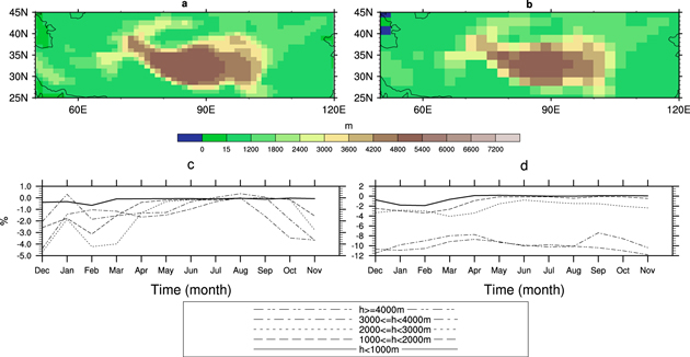
Figure 1. Topography of the study domain (25°–45°N and 50°–120°E) in (a) CCSM4 and (b) GFDL models. Change in monthly surface albedo (%) between late 21st century (2079–2100) and early 21st century (2009–30) averaged over the study area for different elevation bands for (c) CCSM4 and for (d) GFDL models.
Download figure:
Standard image High-resolution imageWe use the Community Climate System Model version 4 (CCSM4) and Geophysical Fluid Dynamics Laboratory (GFDL) coupled general circulation model (CM3) as they have different spatial resolutions and different global sensitivities to climate change. Since the resolutions of the GFDL (2° × 2.5°) and CCSM4 (0.94° × 1.25°) models are different, CCSM4 has more pixels than GFDL for different elevation bands (table 1). GCMs cannot represent the detailed topography which varies between sea level and approximately 9000 m in our domain (see figures 1(a) and (b)). Since the highest elevations in CCSM4 and GFDL are only 5280 m and 5116 m, respectively, the models are limited in their ability to examine feedbacks at the very highest elevations. In the latitudinal band within which our study region is located, all but one of the CMIP5 models find minimum winter temperatures increasing faster at higher elevations, and the GFDL model is at the higher end of the response and CCSM4 at the moderately low end (Rangwala et al 2014). Therefore, we choose these two models to investigate the consistency of their future temperature projections and the role of the snow-albedo feedback in these diverse and complex topographic regions. It would be useful to extend this analysis to other models in the future.
Table 1. Number of pixels under different elevation bands for two models CCSM4 and GFDL.
| CCSM4 | GFDL | |
|---|---|---|
| <1000 m | 497 | 127 |
| 1000–2000 | 366 | 101 |
| 2000–3000 | 100 | 26 |
| 3000–4000 | 69 | 21 |
| 4000–5000 | 124 | 25 |
| >5000 | 41 | 8 |
| Total | 1197 | 308 |
Su et al (2013) compared the simulations of temperature and precipitation over the Tibetan Plateau from 24 of the CMIP5 climate models with meteorological station observations for 1961–2005. The models' climatological annual means as well as their seasonal and spatial variations of temperature, are consistent with observations (Su et al 2013), although there was a cold and wet bias in the multi-model mean in both IPCC AR4 and CMIP5 simulations. This suggests that the models still have some common deficiencies (Su et al 2013), possibly related to their coarse horizontal resolution that limits their ability to resolve the regional topographic variability. Since the maximum cold bias was found in winter, Su et al (2013) suggested that deficiencies in the models' snow-albedo feedback process could also be a factor.
Model description and methodology
CCSM4 has been improved over the previous version (CCSM3) (Gent et al 2011). The hydrologic scheme now includes a new determination of SNC fraction, snow burial of vegetation, and snow compaction parameterizations. An improved treatment of SA and radiation physics of the snowpack has been incorporated, particularly through the inclusion of the snow, ice, and aerosol radiative model (Gent et al 2011). Ghatak et al (2012) (figure 1 in their paper) showed that the fractional SNC simulated by the Community Atmospheric Model version 3 (CAM3) coupled to the community land model (atmospheric and terrestrial components of CCSM4) matches well with the climatology of NOAA-NESDIS visible band snow extent observations. The spatial pattern of the SNC climatology simulated by CCSM4 is consistent with the observed snow extent climatology (result not shown here). GFDL CM3 has also been improved from its previous version as a new land-surface model (LM3) coupled to the atmospheric model (AM3) has been used for terrestrial water, energy and carbon balances (Donner et al 2011). A multi-layer model for snowpack has been used over the soil, and snow and ice albedo are treated more realistically than before (Donner et al 2011). Furthermore, we compared the patterns of each model's monthly surface snow amount (result not shown here) with the SNC climatology (http://climate.rutgers.edu/snowcover/) and found that they are similar to climatology in winter and spring with most of the snow to the west, Southwest, and Southeast of the Tibetan Plateau and generally less snow in the Central Plateau. Both CCSM4 and observations have a pronounced seasonal cycle with little snow in summer, while GFDL still retains much of the snow in summer.
We analyze monthly SNC (%), SA (%), SAT (°C), surface absorbed solar radiation (ASR, W m−2) and cloud cover (CLT, %) between 2006 and 2100. SNC is not available in the archives for the GFDL model and is not shown. We use model simulations from greenhouse gas emission scenario—Representative Concentration Pathways (RCPs) 6.0 which means a radiative forcing of 6 W m−2 by the end of the 21st century (van Vuuren et al 2011). RCP 6.0 is considered to be a medium baseline greenhouse gas emission scenario among the four RCPs. We show results for spring (March–April–May) based on the ensemble means of CCSM4 and GFDL which have six and one ensemble runs respectively.
In order to determine changes in SA and SAT between the late and early 21st century, we use 2079–2100 climatology as the late 21st century and 2009–30 climatology as the early 21st century. Scatter plots are used to examine the correlation between variables. Furthermore, we employ linear trend analysis and assess the statistical significance of the regression coefficients at the 5% level of confidence, using student's t test (Helsel and Hirsch 1992). We employ an empirical orthogonal function (EOF) analysis which is a widely used multivariate statistical technique used for data compression of large space–time fields. The data compression creates new variables that are linear combinations of the original variables (Wilks 2006). The advantage of this method is that the spatial and temporal variability of the variables are described through the statistical 'modes' (Emery and Thompson 2001). We employ this method through the decomposition of the covariance matrix to create pairs of spatial maps and principal component timeseries that explain the fraction of the total variance in the field, with the first mode explaining the highest variance of the field. Here, we present the regression maps of each field instead of showing mode maps and principal component timeseries, similar to Deser et al (2000). The regression maps are obtained by calculating the linear regression coefficients between the timeseries of the original field at each grid point and the leading principal component timeseries of the corresponding field. Then we multiply the value at each grid cell with the linear trend of the leading principal component timeseries. These regression maps provide more meaningful units than EOF modes, and they explain the change in each original field with respect to the linear trend in the leading EOF mode of the corresponding field.
Results
Figures 1(c) and (d) show that there are significant elevational differences in the changes in monthly SA during the 21st century (years 2079–2100 minus years 2009–30). For CCSM4, the changes in albedo are correlated with changes in SNC so that decreases in albedo imply decreases in SNC. Since GFDL does not provide SNC as an output variable, we can't do the same correlation. For GFDL, SA decreases more at the highest elevations in all months. For CCSM4, SA decreases more at the highest elevations in spring and autumn and more at the lowest elevations in winter. In fact, the rate of decrease for CCSM4 in spring is reduced somewhat because there are some grid cells in the higher elevation Western Tibetan Plateau where SNC actually increases. For the lowest elevations in both models, SA decreases in winter by approximately 3% and is unchanged from April through October, primarily because there is no SNC there except in winter. At the highest elevation, the maximum decrease of albedo occurs in December for CCSM4 (∼4–5%) and in November/December for GFDL (∼11–12%). In some of the highest elevation regions, there may not be a reduction in albedo during winter as these regions will remain too cold for the snow pack to melt.
Spring is the transitional season when SNC is most vulnerable to changes in radiation and SAT because of its effect on snowmelt; thus, it is the season when the snow-albedo feedback is likely to be most effective. The incoming solar radiation in spring increases as the solar elevation angle becomes higher, unlike autumn when the angle becomes lower. We therefore focus on spring in the remainder of this paper. The temporal evolution of spring SA, SNC and SAT during the 21st century over high and low elevation regions is shown in figure 2. Temperature is increasing at both high and low elevations for both models, but the increase is greater for the GFDL model which is consistent with its higher global sensitivity. The range of changes in SAT and SA is significantly higher for GFDL than for CCSM4, particularly at high elevations. Table 2 shows that there is little difference between the warming rates at high and low elevations for the CCSM4 model, but that the warming rates are enhanced at higher elevations in the GFDL model. There is a general decrease in SNC and SA in high elevation regions in CCSM4 and in SA in GFDL simulations (figure 2). Both models show little change in SA at low elevations, primarily because many of the grid cells there have little or no snow initially. Figure 2 and table 2 show that SA is correlated with SAT at high elevations in both models, but not correlated at low elevations where there is little snow. We next examine the correlation between SAT and SA at each grid cell.

Figure 2. Timeseries of spring (MAM) snow cover (blue), surface albedo (red) and surface air temperature (black) for the 21st century averaged over the study region for different elevation bands for CCSM4 (left). Same for GFDL (right) except snow cover is not available. Thin lines are seasonal timeseries and thick lines are five year running means.
Download figure:
Standard image High-resolution imageTable 2. Top two rows show linear regression coefficients for spring surface air temperature (°C/decade) and surface albedo (%/decade) over the study region between 2006 and 2100 for different elevation bands. Bottom two rows show Pearson correlation coefficients (R) for spring surface albedo versus surface air temperature and for snow cover versus surface air temperature during 2006 and 2100 time period for different elevation bands. Slopes and correlation coefficients significant at 95% confidence level are shown in bold. Regression coefficients in bold font have p-value less than 0.001. Standard error of regression coefficients has been provided in parentheses.
| MAM | |||||||||||
|---|---|---|---|---|---|---|---|---|---|---|---|
| Elevation | h < 1000 | 1000< = h < 2000 | 2000< = h < 3000 | 3000< = h < 4000 | h> = 4000 | ||||||
| Model | CCSM4 | GFDL | CCSM4 | GFDL | CCSM4 | GFDL | CCSM4 | GFDL | CCSM4 | GFDL | |
| m | SAT | 0.23 | 0.37 | 0.24 | 0.38 | 0.24 | 0.42 | 0.22 | 0.42 | 0.23 | 0.47 |
| (0.010) | (0.027) | (0.012) | (0.032) | (0.014) | (0.033) | (0.012) | (0.029) | (0.014) | (0.036) | ||
| SA | −0.01 | −0.01 | −0.05 | −0.17 | −0.16 | −0.46 | −0.18 | −1.22 | −0.27 | −1.27 | |
| (0.002) | (0.010) | (0.008) | (0.034) | (0.021) | (0.079) | (0.027) | (0.096) | (0.044) | (0.153) | ||
| r | SA versus SAT | −0.214 | −0.376 | −0.613 | −0.765 | −0.809 | −0.809 | −0.809 | −0.888 | −0.823 | −0.865 |
| SNC versus SAT | −0.418 | — | −0.640 | — | −0.856 | — | −0.900 | — | −0.903 | — | |
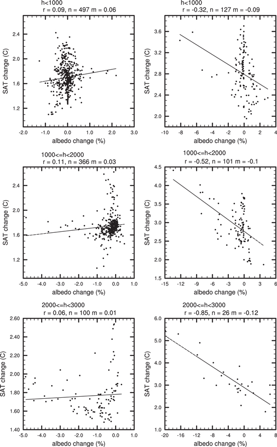
The relationship between changes in SA and changes in SAT in spring for the two models is shown in figure 3. Changes in each of these variables during the 21st century (2079–2100 minus 2009–30) are calculated for different elevation bands. Each point on the scatterplots represents the value at a specific grid cell. There are more grid cells for CCSM4 than GFDL because of its higher resolution. The correlation between these two variables is apparent in CCSM4 at and above 3000 m and for GFDL at 2000 m and above. The slope of the linear regression fit as well as the correlation coefficients is higher for GFDL in most elevation bands. However, at and above 4000 m, CCSM4 exhibits the highest correlation and slope between these two variables. Although the change in SAT and SA is much greater for the GFDL model than CCSM4, the slope of the linear regression fit is the same for both models at 4000 m and above (−0.1 °C/%). For CCSM4, figure 3 also shows that changes in SA for individual grid cells above 4000 m can be positive, negative, or unchanged. Furthermore, a spatial plot (not shown) of the changes in SA, SAT and SNC during the 21st century indicates that there are grid cells in the Western Tibetan Plateau where snow increases in spring, which in turn leads to an increase in SA and reduction of the warming rate relative to the surrounding regions.
Download figure:
Standard image High-resolution image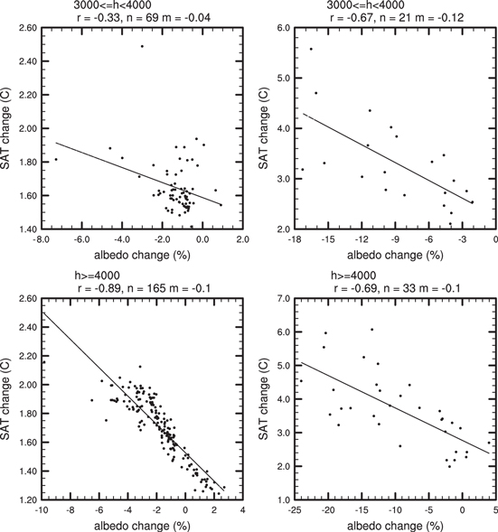
Figure 3. Relationship between changes in spring (MAM) surface albedo (%) and surface air temperature (°C) between the late 21st century (2079–2100) and early 21st century (2009–30) for CCSM4 (left) and GFDL (right) models for different elevation bands.
Download figure:
Standard image High-resolution imageIn summary, figure 3 confirms that the increase in SAT at high elevations is highly correlated with decreasing SA. We have also examined how the snowline and the elevation of the 0 °C isotherm vary with time (figure 4). The average elevation of the spring 0 °C isotherm (defined here as any pixel with average spring SAT between −1 °C to 1 °C) is approximately 3200 m and 2500 m for CCSM4 and GFDL respectively in 2006; although there is local variability. The models indicate that this elevation increases for CCSM4 and GFDL by the end of the century as the snowline retreats. Note that the number of pixels where average spring SAT is between −1 °C and +1 °C is low for GFDL due to its coarse resolution. The linear slope of the timeseries showing the average elevation of the 0 °C isotherm as a function of time is greater for GFDL than CCSM4 (∼12 m/year in GFDL versus ∼7 m/year in CCSM4). Thus, the loss of SNC (also shown in figure 2) causes a reduction of SA, an increase in the surface ASR, and contributes to the high correlation between changes in SA and SAT, as well as the enhancement of warming rates at higher elevations. We cannot easily quantify the magnitude of the snow-albedo feedback mechanism because we would expect a high correlation between changes in SAT and SA since increasing temperatures cause snow to melt thus decreasing SA. However, a prominent role for the snow-albedo feedback mechanism is suggested in regions where the warming rate is greater than in the surrounding areas. To investigate this spatial variability, we next perform an EOF analysis.
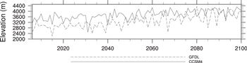
Figure 4. Timeseries of the average elevation (m) of the 0 °C isotherm in spring defined as the average elevation of grid cells with average spring SAT between −1 °C and 1 °C between 2006 and 2100 for CCSM4 and GFDL.
Download figure:
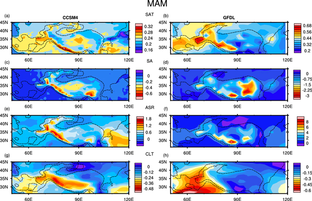
Standard image High-resolution imageFigure 5 shows the results associated with the leading mode of EOFs of SAT, SA, ASR and CLT which are driven primarily by the temporal trends in most of these fields since the data have not been detrended. The correlation of the leading EOF modes of SAT, SA, ASR and CLT between CCSM4 and GFDL are 0.77, 0.54, 0.42 and −0.06 respectively. The dominant EOF mode of spring SAT explains ∼78% and ∼56% of the total variance in CCSM4 and GFDL respectively. Positive regression coefficients associated with the linear trend in the first mode of the principal component time series of spring SAT in both models show an overall positive trend for the 21st century (figures 5(a) and (b)). The large and positive regression coefficients over the Himalayas, Karakoram, Pamir, and Central Asian mountain ranges suggest amplified warming in the higher elevation regions. Thus, the leading EOF mode explaining the highest variance of the SAT field clearly shows amplified warming over high elevation regions, particularly in the high mountains to the Southwest and West of the Tibetan Plateau where the topography gradient is maximum.
Figure 5. (a) and (b) Maps show the linear regression coefficient at each grid cell calculated by regressing the spring (MAM) surface air temperature field onto the first principal component time series of surface air temperature and then multiplying by the linear trend in the corresponding principal component timeseries for CCSM4 (left) and GFDL (right) models. Other panels are the same as (a) and (b), except for (c) and (d) surface albedo, (e) and (f) absorbed solar radiation, and (g) and (h) cloud cover. 1000 m and 2000 m elevation contours are superimposed on each regression map. Units are (a) and (b) °C/decade, (c) and (d) %/decade, (e) and (f) W m−2/decade and (g) and (h) %/decade.
Download figure:
Standard image High-resolution image
The dominant mode of SA explains about 35% of the total variance in both models; whereas, the leading mode of ASR explains 27% and ∼23% of the total variance in CCSM4 and GFDL, respectively. Negative regression coefficients in figures 5(c) and (d) associated with the linear trends in the first mode principal component timeseries are interpreted as decreasing SA in the high elevation regions. Although the spatial pattern of amplified warming collocates with the spatial pattern of decreasing SA as appeared in the leading EOFs in both models, the former extends more to the South over the Himalayas and over the Karakoram in CCSM4. Additionally, SA decreases over part of the Eastern Tibetan Plateau where an increase in SAT is not apparent in the leading EOF pattern.
Figures 5(e) and (f) show that the ASR is increasing in the same regions where the SA is decreasing in the two models. The leading principal component timeseries of SA and ASR are highly correlated with each other as well as with the first principal component SAT timeseries in both models (table 3). The EOF analysis of SAT, SA and ASR indicates that albedo decreased owing to the loss of SNC which in turn leads to an increase in ASR, which is centered over the Central Asian mountains, the Himalayas, the Karakoram and Pamir where amplified warming is also visible. However, there are some areas, such as the Eastern Tibetan Plateau and a very high elevation band (greater than 4000 m) over the Karakoram and the Himalayas, where amplified warming is not apparent in spite of a significant decrease of SA. To investigate this further, we next perform the same EOF analysis on CLT.
Table 3. Correlation coefficients between leading PC timeseries of different variables from CCSM4 and GFDL. Correlation coefficients significant at 95% confidence level are shown in bold.
| CCSM4 | GFDL | |
|---|---|---|
| SAT versus SA | −0.78 | −0.79 |
| SAT versus ASR | 0.71 | 0.80 |
| ASR versus SA | −0.85 | −0.92 |
| CLT versus SA | 0.82 | −0.26 |
Figure 5(g) shows that the negative regression coefficients associated with the linear trend in the dominant mode of spring CLT in the CCSM4 model indicates decreasing CLT over the same region where ASR is increasing, which suggests that the increasing ASR there is occurring in response to the combined effects of decreasing SA and decreasing CLT. For the GFDL model, there is no trend in the first EOF mode of CLT, which is consistent with the low correlation coefficient between the dominant EOF mode of CLT versus SA in GFDL shown in table 3.
Conclusions and discussion
We have investigated projected changes in SAT in the Himalayas, Karakoram, Tibetan Plateau, Central Asian mountains and surrounding regions (25°–45°N; 50°–120°E) during the 21st century using two different GCMs from the CMIP5 archive (CCSM4 and GFDL). This region includes a wide variety of topography with elevations ranging from near sea level to about 9000 m. The principal focus is on the role of the snow-albedo feedback on the amplified warming at higher elevations relative to lower elevations, primarily during spring. We use two models with different spatial resolutions and somewhat different global sensitivities to climate change to investigate whether the projected changes and relationships between variables are similar in our study region.
As expected owing to their different sensitivities to climate change for the mid-latitude band that includes our study region, the rate of temperature change in our study region is greater for the GFDL model than for CCSM4 (0.23 °C/decade in CCSM4 versus 0.45 °C/decade in GFDL at and above 4000 m elevations in spring). During the 21st century, both models show that there is an overall decrease in SA that is significantly amplified at the higher elevations. The decrease of SA owing to the loss of SNC is consistent with the retreat of the 0 °C isotherm in both models. The decrease in albedo is much smaller for CCSM4 than for GFDL in all seasons (e.g., −0.27%/decade in CCSM4 versus −1.27%/decade in GFDL in spring at and above 4000 m elevations), and this might be expected from its correspondingly smaller increase in temperature. However, when we examine the response of SAT to changes in SA, we find that they are same (−0.1 °C/%) in GFDL and CCSM4 at 4000 m and above in spite of the models' temperature changes being quite different during the 21st century. One of the implications of these results could be that the differences in global sensitivities to the climate change of the two models could be related to how they treat snowpack, snow melt and the associated snow/albedo feedback in their 21st century simulations. One of the limitations of this analysis is that the mean topography in both models is well below 9000 m which is the approximate level of the highest peaks, so we cannot resolve enough elevation bands above 4000 m to confirm our results at the very highest elevations for this region.
An EOF analysis is used to compare the spatial and temporal patterns of variability for the two models. The dominant EOF modes from both models clearly show amplified warming over high elevation regions, such as the Central Asian mountains, the Himalayas, the Karakoram and Pamir during spring. The leading spatial and temporal patterns of the EOF analysis of SAT, SA and ASR are consistent for the two models, although CLT is not. Much of the enhanced warming tends to occur in regions where the elevation gradients are greatest. The decrease in SA and the associated increase in ASR are apparent over the above-mentioned regions where there are enhanced rates of temperature increase. In these same regions, the increase in ASR is a result of both loss of CLT and snow pack during spring; but the impact of CLT is only found in CCSM4. There are, however, some areas in the leading EOF mode such as the Eastern Tibetan Plateau and a very high elevation band (greater than 4000 m) over the Karakoram and the Himalayas where enhanced warming does not occur even though SA is decreasing and ASR is increasing.
These results are consistent with the modeling study of Rangwala et al (2013) which showed how amplified warming over high elevation regions including the Tibetan Plateau and surrounding region relative to low elevations is apparent in current GCM simulations under all RCP scenarios. Furthermore, we show that snow-albedo feedback is a contributing factor in this amplified warming, as suggested by Pepin and Lundquist (2008) and Liu et al (2009). Other processes that have been suggested for amplified warming at high elevations include increases in DLR caused by increasing atmospheric water vapor (Rangwala et al 2010), changes in CLT (Duan and Wu 2006), and changes in atmospheric circulation (Liu et al 2009 and Li et al 2012). Our study indicates that the snow-albedo feedback is a contributing factor to elevation dependent warming, however questions remain about its relative importance among these other processes which may vary seasonally. In most cases there will not be a single process responsible for elevation dependent warming, but rather an interplay among multiple factors that lead to either amplification or reduction of the rate of increase in SAT and create complex spatial signatures of the response.
Acknowledgements
This project has been supported by NSF grants 1064281 and 1064326. Debjani Ghatak is grateful to the Rutgers Institute of Marine and Coastal Sciences for post doctoral support, as well as to NASA MEaSUREs award NNX08AP34A and the above NSF grants. This project also received support from the New Jersey Agricultural Experiment Station and the USDA-National Institute for Food and Agriculture, Hatch project number NJ32103. We thank Catherine Naud, Imtiaz Rangwala and Yonghua Chen for helpful discussions and comments. We sincerely thank two anonymous reviewers whose comments led to significant improvements in the original manuscript.