
Abstract
The North Atlantic Oscillation (NAO), the East Atlantic (EA) and the Scandinavian (SCAND) modes are the three main large-scale circulation patterns driving the climate variability of the Iberian Peninsula. This study assesses their influence in terms of solar (photovoltaic) and wind power generation potential (SP and WP) and evaluates their skill as predictors. For that we use a hindcast regional climate simulation to retrieve the primary meteorological variables involved, surface solar radiation and wind speed. First we identify that the maximum influence of the various modes occurs on the interannual variations of the monthly mean SP and WP series, being generally more relevant in winter. Second we find that in this time-scale and season, SP (WP) varies up to 30% (40%) with respect to the mean climatology between years with opposite phases of the modes, although the strength and the spatial distribution of the signals differ from one month to another. Last, the skill of a multi-linear regression model (MLRM), built using the NAO, EA and SCAND indices, to reconstruct the original wintertime monthly series of SP and WP was investigated. The reconstructed series (when the MLRM is calibrated for each month individually) correlate with the original ones up to 0.8 at the interannual time-scale. Besides, when the modeled series for each individual month are merged to construct an October-to-March monthly series, and after removing the annual cycle in order to account for monthly anomalies, these correlate 0.65 (0.55) with the original SP (WP) series in average. These values remain fairly stable when the calibration and reconstruction periods differ, thus supporting up to a point the predictive potential of the method at the time-scale assessed here.
Export citation and abstract BibTeX RIS

Content from this work may be used under the terms of the Creative Commons Attribution 3.0 licence. Any further distribution of this work must maintain attribution to the author(s) and the title of the work, journal citation and DOI.
1. Introduction
Renewable energies constitute a major stake within the mitigation strategies aimed at facing climate change (IPCC WG III 2007). This latter affects particularly southwestern Europe (Giorgi 2006), with the Iberian Peninsula having experienced a recent increase in climatic extremes such as heatwaves and droughts (Della-Marta et al 2007, Vicente-Serrano and Cuadrats-Prats 2007, García-Herrera et al 2010).
Both Iberian countries (Portugal and Spain) have emerged in the forefront of renewable energy production, investing considerably in new renewable energies installations during the last decade, with a prominence of wind farms (Río González 2008) but more recently also solar plants (Ridao et al 2007), mainly using photovoltaic systems while concentrating solar power systems are still in a nonmature stage with weak penetration (Lilliestam et al 2012). This commitment does not result solely from an environmental motivation, as exposed above, but it has also an economical dimension (Apergis and Payne 2010). Iberia is still very dependent on imports of energy from abroad to supply its energy demand (Bhattacharyya 2009, Bilgin 2009), which has associated very high costs. The exploitation of the indigenous renewable potential helps to alleviate this, promoting, furthermore, the local employment (Moreno and López 2008, San Cristóbal 2011).
The success of the investments in the renewable energy sector requires thorough evaluations of the weather and climate-dependent resources, including their variability and potential predictability at various time-scales, from meteorological to climatic (Brayshaw et al 2011, García-Bustamante et al 2013). The main difficulty for such evaluations is related to the inadequacy of lengthy, good quality and spatially dense observational databases. Fortunately, nowadays the availability of sufficiently accurate high-resolution climate simulations can help to overcome this limitation, at least partially (Tapiador 2009, Heide et al 2010, Jerez et al 2013b).
It has been highlighted that a large part of the European climate variability is controlled by just a few large-scale circulation patterns (Trigo et al 2008). The North Atlantic Oscillation (NAO) has been the focus of many works unveiling its role on the precipitation, cloudiness or wind fields among others (Hurrell 1995, Trigo et al 2002, 2004, Pozo-Vázquez et al 2004, López-Moreno and Vicente-Serrano 2008, Martín et al 2010, Brayshaw et al 2011, Jerez et al 2013b). Other modes may have received less attention, although their impacts have been also reported. In particular, the East Atlantic (EA) and the Scandinavian (SCAND) modes have demonstrated influence on the Iberian climate (Paredes et al 2006, Trigo et al 2008, Martín et al 2010, Ramos et al 2010). However, none of these studies pays special attention to the renewable potential of Iberia and its variations according to the phase of those large-scale circulation modes, and most of them are based on either coarse or sparse databases, with the exception of Jerez et al (2013b) that also includes an analysis based on measured power generation data, although focuses only on the NAO.
Hence, taking advantage from a 49-years long hindcast climate simulation with a homogeneous resolution of 10 km over the target region, the aim of this work is to deepen the understanding of the extent at which NAO, EA and SCAND determine the solar (photovoltaic) and wind power generation potential (SP and WP respectively) in the Iberian Peninsula, including the assessment of their suitability to be used as predictors.
2. Data
2.1. Solar and wind potential
The SP and WP series analyzed here were derived from primary data of surface short-wave downward radiation (SWD) and wind speed (WS) obtained from a hindcast regional climate simulation performed with the mesoscale model MM5 (Grell et al 1994) driven by the ECMWF ERA40 reanalysis (Uppala et al 2005) and analysis data. This simulation covers the whole Iberian Peninsula with a 10-km resolution homogeneous grid and spans the period 1959–2007 with hourly resolution, and has demonstrated skill for reproducing accurately the spatial and temporal variability of meteorological variables such as wind speed and direction, precipitation and maximum and minimum daily temperature, at least at the monthly time-scale (Jerez et al 2013b). Unfortunately, we could not validate similarly the accuracy of the simulated surface solar radiation due to the lack of observations at our disposal.
Following the set of rules proposed by Ruiz-Arias et al (2012), the series of SWD and WS were transformed into series of SP (considering only the photovoltaic technology as it is the most widely used) and WP respectively (equations (1) and (2)). In equation (1), GSTC refers to the incoming surface short-wave radiation at standard test conditions (which is 1000 W m−2) and PR is the performance ratio accounting for system losses (typically 0.75). For the transformation of WS into WP (equation (2)), we considered the cut-in, cut-off and rated speeds (SI,SO and SR respectively) specified for the GAMESA (www.gamesa.es) wind turbine model G87 (i.e. SI = 4 m s−1,SO = 25 m s−1 and SR = 12 m s−1), one of the most used in Iberia. The vertical layer of the simulation being closest to its tower height (87 m) corresponds to an altitude of about 100 m. Given that the relationship between WS and WP expressed in equation (2) is not linear, it is particularly valuable the hourly resolution of the WS data used here (at coarser time-scales, e.g. monthly, equation (2) may not be valid).
Note that SP and WP, as they are considered here, are normalized (dimensionless) values representing the power generation potential (sometimes simply referred to as potential). The power generation would be the product of these values of SP or WP and the installed capacity power that we have for each resource. Hence, SP and WP range between 0 (no generation potential) and 1 (the power generation would equal the installed power capacity).
2.2. Large-scale climatic indices
The values of the NAO, EA and SCAND indices for the whole simulated period were retrieved from the Climate Prediction Center (CPC) of the NOAA (www.cpc.ncep.noaa.gov) at the finest temporal resolution available for each: daily for the NAO index and monthly for EA and SCAND.
3. Methodology
3.1. Temporal correlation
Temporal correlation (r), computed through the Pearson coefficient, is used to measure the strength and linearity of the relationship between the large-scale circulation indices and the renewable power generation potential series.
3.2. Composites
The impact of the various modes on SP and WP is quantified through composites showing the difference (Δ) in their mean values between the positive (>0.5) and negative (< − 0.5) phases of the NAO, EA and SCAND indices (as in Jerez et al 2013b). These differences are given as percentage with respect to the climatology of the assessed magnitude (e.g. equation (3)). Note that the value of Δ would increase with higher thresholds in the definition of the positive and negative phases of the indices (since we would be considering more extreme cases). However, this would reduce the number of events averaged in each case and thus higher values of Δ would be required for achieving statistical significance. The subjective threshold of 0.5 was chosen by pondering both issues.

3.3. Multi-linear regression model
In order to investigate the extent at which NAO plus EA plus SCAND are able to explain the temporal evolution of the SP and WP series, we use a multi-linear regression model (MLRM) including the three large-scale circulation indices as predictors (equation (4)), hence taking into account their joint influence. First, in order to obtain the values of the coefficients C0,CN,CE and CS, we calibrate the MLRM by fitting the original SP and WP time-series to equation (4) using the minimum mean square error method. Second, we use these values to reproduce, with equation (4), the SP and WP series according to the variations of NAO, EA and SCAND. The accuracy of these modeled series is then evaluated by comparison with the original ones. To this end, we use two scores: the temporal correlation (r) between the original and the modeled series, and the standard deviation ratio (stdr) defined as the ratio between the standard deviation of the modeled series and the standard deviation of the original series.

4. Results
4.1. Time-scale varying correlations
The availability of daily records of NAO makes it possible to assess its influence on SP and WP at a wide range of time-scales. We have computed the temporal correlation between the NAO index and SP/WP using daily, weekly, monthly, seasonally and yearly averaged series (figures 1(a) and (b)). Similarly, the correlation between EA/SCAND and the resources was computed at time-scales ranging from monthly to yearly (figures 1(c)–(f)). In this analysis we have considered either all the records in the series or only those corresponding to the different seasons or months. This approach allows to identify both the time-scale and season of the year with maximum influence of each mode on the resources. This analysis was done for each grid-point of the domain, but we opted to present here spatially averaged series of SP and WP for simplicity. These series were obtained by averaging spatially over those land grid points showing significant correlation values between the resources and the climatic indices. We have indicated in figure 1 if the fraction of grid points averaged in each case exceeds 30% or 50% of the total number of land grid points of the Iberian Peninsula.
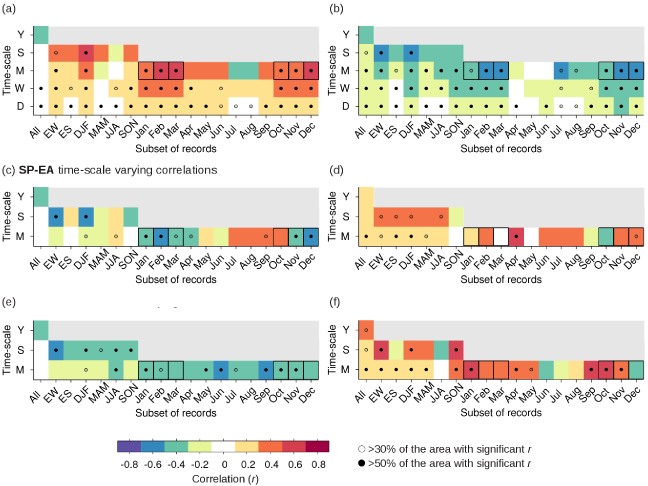
Figure 1. Temporal correlation (r) between modes (NAO ((a), (b)), EA ((c), (d)) and SCAND ((e), (f)) indices) and resources (SP ((a), (c), (e)) and WP ((b), (d), (f))) at various time-scales and considering various subsets of records of the whole series. Daily (D), weekly (W), monthly (M), seasonally (S) and yearly (Y) averaged series are considered (y-axis), when possible (EA and SCAND indices are only available at the monthly and longer time-scales). In each case we have considered all the records in the series (All), but also, when it makes sense (when not colored in gray), only those records corresponding to each one of the four seasons (winter, i.e. DJF; spring, i.e. MAM; summer, i.e. JJA; and autumn, i.e. SON), and only those corresponding to each one of the twelve months (from January to December). This is indicated in the x-axis. The series of SP and WP considered are spatially averaged series involving those land grid points within the IP where the correlation between the indices and the resources is significant (p < 0.05). An empty (solid) circle denotes that the size of this area represents more than a 30% (50%) of the whole land area of the IP. Black squares indicate the case studies that were further investigated.
Download figure:
Standard image High-resolution imageSignificant correlations are obtained at every time-scale for both SP and WP series and NAO, often over more than 50% of the Iberian Peninsula area. Worth mentioning, Jerez et al (2013b) showed indeed significant correlation between the NAO index and measured series of solar and wind power generation in Spain at the yearly time-scale (these public data are not available at finer time-scales with sufficient length). However, according to figure 1, the strength of the correlations is maximum at the monthly time-scale for the months of the winter half of the year (within the range 0.5–0.7, with positive values for SP while negative for WP) in comparison to larger (seasonal, yearly) and smaller (daily or weekly) time-scales. The greatest influence of NAO in winter may reflect the fact that local processes, such as land–atmosphere interactions, gain relevance in summer (Jerez et al 2012) and can mask to some extent the influence of the large-scale circulation. However, both EA and SCAND not only show similarly high and widespread correlations with the monthly series of SP and WP in the winter months (although with opposite sign than the correlations with NAO in each case), but also in some months of the summer half of the year (figures 1(c)–(f)). For example, SP and SCAND show maximum correlation in June and WP and EA in April.
Noteworthy, the strength and even the sign of the correlation between modes and resources differ from one season to another. This explains that, although high correlations still appear at the seasonal time-scale for some seasons (mainly winter, i.e. for the DJF-averaged series), they are less appreciable at the annual time-scale.
Therefore, the optimum approach to characterize the impact of these large-scale circulation modes on SP and WP consists on analyzing it at the monthly time-scale and, given the differences among the various months along the year, for each month separately. In other words, these modes appear to play a major role on the interannual variations of the monthly mean values of SP and WP, particularly during the winter half of the year, thus representing a major low-frequency (within the context of this analysis) driving factor for both of them.
Following such approach, we have focused on the October-to-March months in the following sections. The choice of these winter months responds to three reasons: (1) brevity, (2) they showed the highest signals in many cases (see squares in figure 1), and (3) although, contrary to the wind resource, the solar resource is maximum in summer (the wind maxima peaks in winter), both resources present the highest interannual variability in winter (not shown), when thus a better understanding of the underlying causes becomes more relevant.
4.2. Monthly impact patterns
The correlation patterns between the various indices and SP (WP) at the monthly time-scale for each winter month individually are depicted in figure 2 (3) (first-to-third columns, in colors). This analysis further shows noticeable differences both in the magnitude and the spatial distribution of the correlations from one month to another, highlighting that in some places/months these correlations are up to 0.8.
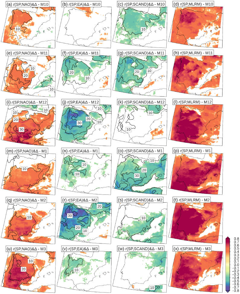
Figure 2. Shaded colors depict the temporal correlation (r) between the SP series and (from left to right) NAO, EA, SCAND and the MLRM-modeled SP series. Correlations are computed at the monthly time-scale for each winter month separately (from top to bottom: October to March). Shown correlations are statistically significant (p < 0.05). Contours depict the difference (Δ) in the mean SP between positive and negative phases of the various indices (in % respect to the mean SP climatology) in the first three columns. Contour interval is 10, starting in 10.
Download figure:
Standard image High-resolution imageIn order to quantify the variations in SP and WP associated to phase changes of the various modes, we computed the difference in the mean values of SP and WP between their positive and negative phases in each month (the number of events averaged in each case is specified in table 1). This difference is provided in percentage with respect to the mean climatology of each resource by contours in the first three columns of figures 2 and 3.
Table 1. Number of positive (+) and negative (−) phases of NAO, EA and SCAND in the October-to-March monthly mean series of their indices in the period 1959–2007.
| October | November | December | January | February | March | |
|---|---|---|---|---|---|---|
| NAO (+/ − ) | 22/14 | 10/17 | 13/16 | 12/21 | 12/22 | 13/20 |
| EA (+/ − ) | 13/20 | 15/18 | 15/22 | 12/20 | 15/16 | 15/19 |
| SCAND (+/ − ) | 22/13 | 16/13 | 17/13 | 14/14 | 17/11 | 18/16 |
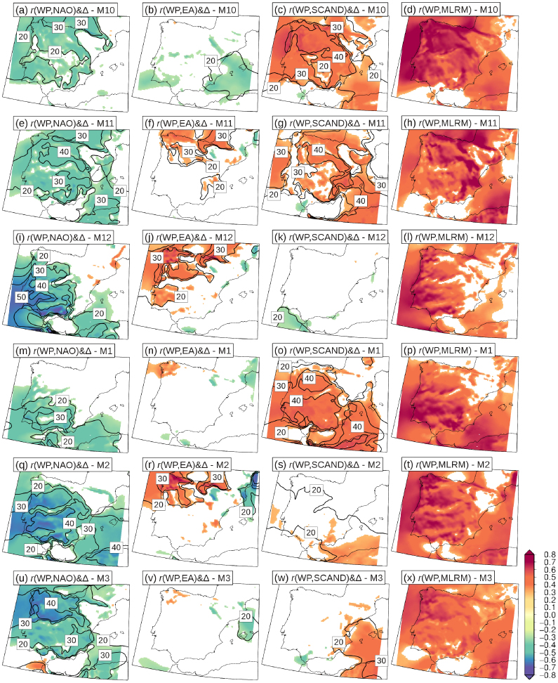
Figure 3. As figure 2 for WP. Contour interval is 10, starting in 20.
Download figure:
Standard image High-resolution imageRegarding SP (figure 2), the signature of NAO is appreciable and statistically significant in every month, although the most significant signals appear in December, February and March. The role of the EA pattern is also very relevant throughout the considered winter months (particularly in November, December and February) although being irrelevant in October. Likewise, the impact of the SCAND mode is quite noticeable in all months with the exceptions of December and March. In general, the strongest signals appear concentrated in western and central sectors, prevailing in the southwestern those associated to NAO and in the northwestern those associated to EA. The impact of SCAND evolves spatially from the northwest in the last months of the year to the southeast in January and February. Variations in mean SP associated to changes in the phase of the indices range from 10% of its climatology to over 30%, although these later are restricted to small areas and observed only for a few months. These signals are attributed to changes in cloudiness, in turn associated to changes in the synoptic flow. Westerly and northwesterly flows advect humid air from the ocean into the Iberian Peninsula, thus promoting the formation of clouds, enhancing precipitation and diminishing the solar radiation that reaches the surface. On the contrary, land-to-ocean flows and the more anticyclonic conditions during some phases of the considered modes have associated clearer skies in terms of clouds and thus enhanced surface downward short-wave solar radiation (Trigo et al 2002, Trigo 2006, Jerez et al 2013b).
Variations in WP (figure 3) reach frequently 30%, mounting up to values higher than 40% in several months associated to phase changes of both NAO and SCAND. As in the case of the solar resource, there are months with feeble signatures from EA and SCAND, while significant signals associated to the NAO phase appear in every month. In this sense, these patterns are similar to those obtained for the solar resource, although depicting different spatial distributions. In particular, the composites for the WP suggest an important role of the orographic factor, with lower values often associated with high mountain ranges and strengthened signals appearing in general within the river valleys. This has been attributed to the fact that in the high lands the wind does not blow through well-defined preferred directions, in contrast to the anisotropy derived from the orographic channeling within the valleys. Hence, as the primary impact of the large-scale circulation patterns on the wind field is on the wind direction, it translates into different wind speeds mainly where changes in the wind direction affect it, i.e. inside the orographic channels (Jerez et al 2013b).
Worth mentioning, the sign of the impact of the various circulation modes on either SP or WP is opposite. While positive NAO phases and negative EA and SCAND phases generally promote SP, the opposite phases of each index enhance WP. This suggests that months expected to be poor (good) in solar production would compensate with increased (decreased) wind production, at least to the extent at which these resources are determined by the aforementioned large-scale patterns.
4.3. Modeling solar and wind potential with NAO, EA and SCAND
The MLRM (equation (4)) was calibrated using the monthly mean series of SP and WP for each winter month individually. The patterns of temporal correlation between the MLRM-modeled series and the original series for both renewable resources are provided in the last column of figures 2 and 3. The results show high correlations (often above 0.8) over most of the Iberian Peninsula for all considered months. The improvement achieved with the MLRM approach in comparison with considering each index individually is noticeable: the strong signals covering almost the entire Iberian Peninsula for most subplots in the last column of figures 2 and 3 stand above those related to each individual mode depicted in the first-to-third columns. Hence, these results prove that the three predictors/indices considered (NAO, EA and SCAND) are not redundant and that, when considered jointly, they are capable of explaining a large fraction of the variability of both renewable resources at this time-scale.
This last result further suggests that NAO, EA and SCAND could be considered for improving the medium-range forecasts of monthly means (i.e. months ahead, given our climatological framework) of the solar and wind potential, as it was similarly stated regarding the usefulness of the NAO for the wind resource in the UK by Brayshaw et al (2011). However, for this purpose it would be desirable that the October-to-March series obtained from merging the individual month series modeled so far, capture well the month-to-month variations of the resources.
We assessed this latter obtaining that the agreement between the original and the modeled October-to-March monthly series of SP and WP (constructed by merging the series modeled for the individual months) is such that r achieves an extremely high value for the SP series (0.96) and a smaller but still significant value in the case of the WP series (0.64) (figures 4(a) and (b)). However, these values are inflated by the inclusion of the seasonal cycle of the series (not removed so far), which is particularly appreciable in the case of the solar resource (figure 4(a)). Thus, we compared the series after removing the annual cycle (figures 4(c) and (d)) obtaining correlation values of 0.67 (0.55) and standard deviation ratios of roughly 0.6 (0.5) for the SP (WP) series. These lower r and stdr values still support the potential of the MLRM for reproducing the temporal variability of the monthly anomalies of the October-to-March series of both SP and WP up to a point.

Figure 4. (a) and (b) depict monthly series (including the months from October to March of each year within the period 1959–2007) of SP (left) and WP (right) averaged for the whole IP. The original series, as they are obtained from the regional simulation, are depicted in black. The series modeled by the MLRM calibrated for each month individually are in colors. The correlation (r) and the standard deviation ratio (stdr) between them is provided. (c) and (d) depict the former series after removing the monthly climatology from each monthly value. (e) and (f) provide Taylor diagrams summarizing the skill of various models to reproduce the original series of either monthly values (the results are represented by solid symbols) or monthly anomalies (the results are represented by empty symbols) of SP and WP. The various models tested (see legend) are described in the text. In particular, the colored symbols correspond to the modeled series depicted with the same color in panels (a)–(d). The cross indicates the position for a perfect model.
Download figure:
Standard image High-resolution image4.3.1. Comparison with simpler approaches.
In order to contextualize the above results, we have compared them with the results obtained with simpler models. Any statistical model should be able to improve the performance obtained with simpler benchmark models such as climatological, persistence or randomness, otherwise it can be considered useless (Wilks 2006). For that, the original monthly series of SP and WP (those shown in figures 4(a) and (b)) were also modeled using: (1) a similar but simpler MLRM calibrated only once using the October-to-March monthly series without considering each month individually (MLRMS), and (2) a reference climatological model assigning to each month the value of its mean climatology (CLIM). As well, the original series of monthly anomalies (shown in figures 4(c) and (d)) were also modeled using: (1) the aforementioned MLRMS (i.e. we remove the climatology from the series obtained with the MLRMS as described above), (2) a MLRM calibrated directly using the series of monthly anomalies, instead of the monthly series, without splitting by months as opposite to the original MLRM approach (MLRMSA), and (3) a reference persistence model that assigns to each time step the value of the original series in the previous time step (PERS). Just to clarify further the procedure, the difference between the MLRMS and the MLRMSA approaches applied to the series of monthly anomalies is that the former is calibrated using the monthly series of absolute SP/WP values (and then we remove the climatology from the modeled series) while the latter is directly calibrated with the monthly series of SP/WP anomalies. In any case the calibration is performed for each month separately but considering the whole October-to-March series; otherwise both models would converge on the original MLRM approach. The results from the various approaches are summarized in the Taylor diagrams (Taylor 2001) of figures 4(e) and (f).
Regarding the modeling of the SP series (figure 4(e)), note that the reference CLIM model (solid black triangle) is pretty close to the MLRM calibrated for each month individually (solid red square). However, this latter still adds some value beyond the climatology as it also reproduces reasonably well the series of monthly anomalies (empty orange square), as commented before. On the other hand, given that the marked annual cycle of the solar resource has nothing to do with the large-scale circulation (being primarily governed by the number of sunshine hours in each month), the MLRMS approach is hardly able to reproduce the October-to-March monthly series of solar potential (solid black circle). It only shows some skill after removing the annual cycle, i.e. in reproducing the series of monthly anomalies (empty black circle). However, for that, it is also worse than the MLRM calibrated for each month individually (empty orange square), which stands always as the best approach, and also than the MLRMSA (empty black diamond). As expected, all models underestimate the variance of the series but for the PERS model (the PERS model consists of the original series with a lag of one time step), which is however not correlated at all with the original series (empty black triangle). This proves that there is not autocorrelation in the original monthly anomalies series.
Similarly, the October-to-March WP series are worse reproduced when the multi-linear regression model is not calibrated for each month separately than when it is; and both reference models (CLIM and PERS) show very poor skill in this case (figure 4(f)). In the case of the absolute monthly series, the CLIM model shows worse skill than for the SP case, hence the improvement of the MLRM in comparison to it is larger in the WP than in the SP case (although its accuracy is more moderate for WP than for SP, figures 4(a) and (b)). On the contrary, the MLRMS approach is not as bad for modeling the WP series as it was for SP, although still less accurate than the MLRM. Actually, since the WP series does not show a marked climatological seasonality within the October-to-March period, it was to be expected the poor reliability of the CLIM model and also the fact that the MLRMS performs better for reproducing the WP series than the SP series. On the other hand, all the tested approaches for modeling the series of WP anomalies show similar results, with r in the range 0.5–0.6 and stdr around 0.5 in all cases. Nonetheless, the added value of the MLRM is also appreciable in this case.
Therefore, the MLRM calibrated for each month individually outperforms both reference models and simpler approaches. This latter further emphasizes the distinct response of the resources to the large-scale climatic variability characterized through NAO, EA and SCAND in each month, and reinforces the advisability of evaluating it for each month individually even if we are interested on reproducing afterward the month-to-month variations of the resources.
4.3.2. Predictive potential.
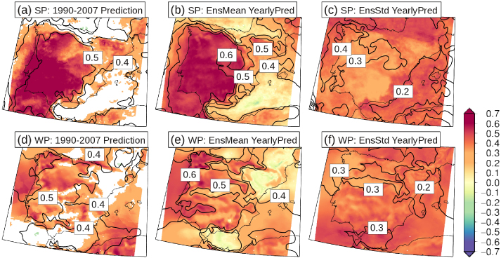
Finally, in order to deepen on the predictive/reproductive potential of the optimum MLRM-based method identified above, we have validated the model using more stringent conditions: different periods for calibration and validation (Wilks 2006). First, we simply used the MLRM calibrated for the period 1959–1989 (for each month separately) to reproduce the SP and WP October-to-March monthly anomaly series of the remaining period 1990–2007. The validation of these modeled series through comparison with the original ones is summarized in figures 5(a) and (d). Second, we adopted the more elaborated leave-one-out approach. For each year within our study period, we reconstructed the October-to-March series of monthly anomalies with the MLRM calibrated using the whole period but excluding that specific year (after removing the records of the corresponding year, the MLRM was calibrated for each month separately as well). Figures 5(b) and (e) provides the means of the values of r and stdr obtained for each single year in this manner, and figures 5(c) and (f) depicts the standard deviation of these sets of r and stdr values. For SP, in both panels (a) (that illustrates the predictive potential of the MLRM with an example) and (b) (that characterizes it statistically) of figure 5, r ranges between 0.6 and 0.7 over wide areas of the western half of the Iberian Peninsula, where the stdr is also well sustained above 0.5 (0.6 in panel (b)). For WP, the results are generally more modest than those for SP, with the highest values of both r and stdr more constrained to western river basins areas, although still reaching values around 0.5–0.6 for r and 0.5 for stdr there (figures 5(d) and (e)). These values agree with those showed in figures 4(c) and (d) and therefore prove that NAO, EA and SCAND can be considered as a set of useful predictors in the time-scale and season assessed here. On the other hand, these patterns (whose spatial distributions resemble to a large extent those obtained in figures 2 and 3) allow to identify the areas with the highest SP and WP predictability based on the large-scale modes. Moreover, figure 5(c) and (f) highlights that the predictability in these areas remains more constant along the study period than in the areas showing lower averaged values of both r and stdr in figures 5(b), (e). This results from the fact that the spread in r and stdr throughout the entire period analyzed is lowest where indeed r and stdr reach the highest values.
Figure 5. (a), (b) r (in all panels by shaded colors, here with p < 0.05) and stdr (in all panels by contours, interval 0.1) values obtained for the SP (upper panels) and WP (bottom panels) October-to-March monthly anomaly series of the period 1990–2007 modeled with the MLRM calibrated (for each month separately) for the period 1959–1989. (b), (e) means of the r and stdr values obtained for the October-to-March monthly anomaly series of each year modeled with the MLRM calibrated (for each month separately) for the whole period but excluding the year to be modeled in each realization. (c), (f) Standard deviation of these latter sets of r and stdr values.
Download figure:
Standard image High-resolution image
5. Conclusions
This work evaluates the extent at which the three major large-scale circulation patterns in the Euro-Atlantic region (NAO, EA and SCAND) determine the solar (photovoltaic) and wind power generation potential over the Iberian Peninsula, considering also their skill as predictors when used in conjunction.
First, we investigated the time-scale in which the influence of these modes on the renewable potential is most noticeable. The largest signals were identified for the interannual variations of the monthly series of the resources (although other time-scales, namely weekly and seasonal, could be also interestingly investigated), depicting different intensity and spatial distribution in each month in both their strength and their spatial distribution. We focused on the winter half of the year (October-to-March months), when the influence of the large-scale circulation on the Iberian climate is generally more relevant (Trigo et al 2008). Besides, both renewable resources present the highest variability in this season, while their maximum values peak either in winter for the wind or summer for the solar resource. Nevertheless, EA (SCAND) also showed strong influence in some spring (summer) months. Hence, although historically (e.g. Trigo et al 2002; Pozo-Vázquez et al 2004), and also in the present study, the attention has been paid to the winter half of the year, future efforts could be worthy devoted to assess summer signals associated to the large-scale dynamics (Cattiaux et al 2013).
Monthly means of SP (WP) vary up to 30% (40%) with respect to its climatology between years with positive and negative phases of the various indices. Worth mentioning, the phases of the various modes promoting the solar resource are the opposite phases enhancing the wind potential, which indicates a plausible temporal complementarity at the time-scale assessed here between both renewable energies (this complementarity is further investigated in Jerez et al 2013a). We should acknowledge that similar findings have been already reported or pointed for the NAO mode alone, although often with much less detail (Trigo et al 2002, Pozo-Vázquez et al 2004, Jerez et al 2013b). On the contrary, to the best of our knowledge, this type of analysis remained largely unveiled regarding the EA and SCAND patterns.
The inclusion of the NAO, EA and SCAND indices in a multi-linear regression model applied to the monthly series of solar and wind potential provided modeled series of these latter that correlates with the original ones up to 0.8 over most of Iberia at the interannual time-scale for every single winter month. This proves that a large fraction of the interannual evolution of the monthly SP and WP series respond, in winter, to the combined influence of these three indices.
Furthermore, not only the interannual variations, but also the month-to-month variations of the resources are acceptably captured by these modeled series, even after removing the climatology (i.e. the month-to-month variations of the monthly anomalies). Objectively, the modeled October-to-March series of monthly anomalies of SP (WP) correlate with the originals 0.65 (0.55) and captures a 60% (50%) of their variability in average. These values remain unaffected when the reconstructed period is excluded from the MLRM calibration period, which proves the predictive potential of the method, especially in western areas.
This last result is particularly valuable in view of some promising works and initiatives aimed at improving the predictability of large-scale climatic indices (Brands et al 2012, Maidens et al 2013) NAO, EA and SCAND, as far as their usefulness to reconstruct SP and WP at the monthly time-scale for the recent past was proved, could constitute a valuable set of predictors to easily anticipate the solar and wind potential in Iberia months ahead in monthly mean terms, as previous works, not for these renewable resources but for other variables, already suggested (e.g. Bierkens and van Beek 2009). This would help to overcome the absence or improve the performance of direct local medium-range climate prediction systems.
Acknowledgments
This study was supported by the Portuguese Science Foundation (FCT) through the project PEST-OE/CTE/LA0019/2013-FCT. The data from the climate simulation, performed under the project Minieólica (PSE.120000.2007.14) funded by the Spanish MEC and FEDER, were nicely provided by the MAR research group from the University of Murcia (Spain). In particular, we want to acknowledge the assistance of Dr Juan Pedro Montávez and Raquel Lorente-Plazas. Last, we would like to acknowledge the feedback provided by three anonymous reviewers, which helped us to improve the quality of this letter.