
Abstract
Wind power introduces variability into electric power systems. Due to the physical characteristics of wind, most of this variability occurs at inter-hour time-scales and coal units are therefore technically capable of balancing wind. Operators of coal-fired units have raised concerns that additional cycling will be prohibitively costly. Using PJM bid-data, we observe that coal operators are likely systematically under-bidding their startup costs. We then consider the effects of a 20% wind penetration scenario in the coal-heavy PJM West area, both when coal units bid business as usual startup costs, and when they bid costs accounting for the elevated wear and tear that occurs during cycling. We conclude that while 20% wind leads to increased coal cycling and reduced coal capacity factors under business as usual startup costs, including full startup costs shifts the burden of balancing wind onto more flexible units. This shift has benefits for CO2, NOX, and SO2 emissions as well as for the profitability of coal plants, as calculated by our dispatch model.
Export citation and abstract BibTeX RIS

Content from this work may be used under the terms of the Creative Commons Attribution 3.0 licence. Any further distribution of this work must maintain attribution to the author(s) and the title of the work, journal citation and DOI.
1. Introduction
Operation of an electric grid depends on dispatchable generating capacity, such as coal and natural gas power plants, which can be cycled in response to variability. Traditionally, variability was largely limited to the demand side. However, an ever-increasing penetration of variable renewable energy technologies, such as wind, promises to increase the amount of cycling performed by dispatchable generators.
APTECH (2009) defined cycling as 'The process of bringing plants on and offline or increasing and decreasing unit output to meet load demand'. Denny (2007) and Valentino et al (2012) used similar definitions. Here we adopted the definition suggested by APTECH and considered cycling operations to include both shutdown–startup cycles, where we differentiated between hot, warm, and cold cycles by the time spent offline; and load cycling, in which output is increased or decreased without shutting down. For reasons discussed later, we focused on shutdown–startup cycles.
As described by Katzenstein and Apt (2009) and Fertig et al (2012), the spectrum of variation introduced by wind generators is not flat across all frequencies. Wind power varies much more at multi-hour than it does at sub-hourly time-scales. Units with small ramp rate limits, such as coal, might therefore be expected to balance much of wind's variability. However, coal plants were by and large designed to provide baseload power Denny (2007), and increased cycling of these plants in response to high wind penetrations could have unforeseen consequences.
Previous work has suggested that using thermal plants to balance wind may result in emissions penalties. Katzenstein and Apt (2009) considered the implications of using a gas + wind + solar combination to produce baseload power. Their findings indicated that ramping a simple or combined cycle gas turbine over its full operating range to balance wind and solar variability resulted in significant emissions penalties for NOX and SO2. The emissions model used by the authors allowed emissions rates to vary with both power output and ramp rate.
Valentino et al (2012) examined the relative contribution of startups to fleet-wide emissions at a range of wind penetration levels. Focusing on the state of Indiana, their results suggested that while cycling increased the emissions rates of individual units, the effect was small compared to the overall emissions reductions that resulted from the displacement of fossil-fueled power by wind power.
Increased cycling of thermal power plants is also likely to result in increased operating costs. Intertek APTECH assessed the cost implications of cycling coal-fired thermal units (APTECH 2009, Shibli et al 2001), while Lefton (2004) and Shibli et al (2001) studied steam units generally. The large and time-varying thermal loads imposed by cycling were found to increase the risk of creep and fatigue damage, with implications for operations and maintenance (O&M) costs, capital maintenance costs, and several other cost categories. Using data from two coal-fired power plants, APTECH (2009) reported that these costs were highest for shutdown–startup cycles and could be on the order of $100 000/cycle. Bentek (2010) suggested that most modeling efforts do not account for the full costs of cycling coal power plants, an omission that might underestimate the costs of integrating wind.
We examined the distribution of startup costs bid into PJM and found that these are far lower than the costs calculated by APTECH, suggesting that actual markets may not fully account for the costs of cycling. The comparison is shown in figure 1. There are several possible reasons for this cycling cost gap. First, it is possible that operators are unable to attribute individual component failures and forced outages to cycling operations. Second, it is possible that while operators are aware of the costs incurred during cycling, market rules do not allow them to include these costs in their bids. While PJM's market rules appear to provide a mechanism to account for startup-related wear and tear in the form of a Start Maintenance Adder (PJM 2012b), it is unclear whether costs of the magnitude suggested by APTECH would gain approval by PJM. Finally, it is possible that operators have concluded that bidding actual startup costs would result in a reduction in their capacity factors and energy market revenues, and are bidding strategically in order to avoid this outcome.
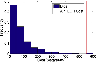
Figure 1. Distribution of cold start costs bid in PJM in 2007 (PJM 2012a) and average APTECH startup cost figures (APTECH 2009, Agan et al 2008), normalized by capacity. The vertical line attributed to APTECH here is the capacity-weighted average of figures for the Harrington and Pawnee plants. The vast majority of startup cost bids far fall below the APTECH figure.
Download figure:
Standard image High-resolution imageThis under-bidding may lead to problems as wind penetration increases. Under current market conditions coal operators may be able to generate sufficient revenues in the energy market to offset the cycling cost gap. However, as wind penetration increases and coal plants are required to cycle more often, profit margins may narrow to the point where cycling costs cannot be recovered. As pointed out by Cullen and Shcherbakov (2010), the operation of an energy market is often sensitive to unit startup costs. Here we determined the increase in coal cycling that could be expected in a high wind penetration scenario in the PJM West area under business as usual startup cost bidding, along with associated emissions and system cost penalties. We then considered low- and high wind scenarios where operators of coal plants bid startup costs at the elevated levels suggested by APTECH.
We constructed a unit commitment and economic dispatch (UCED) model with an hourly time step for the PJM West area, as it existed in 2006. This included the PJM sub-regions of AEP, AP, Dayton, Dominion, and Duquesne. Using simulated wind data generated by the National Renewable Energy Lab (EnerNex Corporation 2011), we considered a scenario with 20% wind energy penetration that approximated compliance with renewable portfolio standards in the region (PJM 2011). To account for the effects of cycling on emissions of CO2, NOX, and SO2, we employed energy penalty curves derived from the EPA's Clean Air Markets data (EPA 2006) and input emissions rates from the National Electric Energy Data System (EPA 2010).
We found that a high level of wind penetration led to a large increase in the cycling of coal units and to an increase in cycling-induced cost and emissions penalties, but that these penalties were small compared to the system-wide savings associated with wind. This finding is consistent with the results of Valentino et al (2012). Furthermore, we found that coal cycling, along with its emissions penalties, was reduced if the full costs of cycling such units were taken into account in operator bids. The high wind with elevated coal start cost scenario was associated with higher normal operations costs, compared to the high wind scenario with low coal start costs, due to fuel switching from coal to gas. Total costs were still lower, however, than in the no-wind case. While incorporating elevated coal startup costs reduced coal unit capacity factors, the combination of reduced startup costs and increased energy prices led to increased aggregate coal unit profitability under the elevated coal start cost scenarios.
2. Methods
2.1. Unit commitment and economic dispatch model
We used a unit commitment and economic dispatch (UCED) model to determine the operating schedule for the PJM West area. The UCED schedules generators so as to meet demand at the lowest possible production cost, subject to unit operating constraints and system security constraints. The operation of the generators in PJM West was modeled day by day over the course of a year. The solution for each day was generated by optimizing over a 48 h period, then stepping forward 24 h. The state of all generators at the end of each day was fed into the next day's optimization in order to enforce ramp rate and minimum up- and down-time constraints across days. The model was formulated as a mixed-integer programming problem and solved using CPLEX.
The UCED model uses generating unit and load data from the PJM West area in 2006. Similar to several other authors, the model does not include transmission constraints (Denny 2007, Valentino et al 2012, Nyamdash et al 2010). This limitation may result in inaccuracies in the amount of cycling performed by particular units, but is unlikely to affect the implications of the aggregate results, as variation in net load determines the amount of cycling that must be performed at the system level. For the high wind case, the UCED attempts to meet net load (load minus available wind plus curtailment) at least cost.
Note that the model was built with the assumption of perfect load and wind forecasts over each 48 h period of model execution. In real power systems, forecast errors lead to the occurrence of short time-scale corrections, mostly performed by fast-ramping units procured through the ancillary service markets, which we did not model. Since this work focused on slow-ramping coal units, we expect this limitation had a minor impact on results as they relate to the operations of coal power plants. A detailed description of the model formulation is included in the supporting information (available at stacks.iop.org/ERL/8/024022/mmedia).
Production costs used in the model include fuel, variable O&M, and startup costs. Fuel costs were calculated at the unit level as the product of power output, heat rate, and utility-delivered fuel price. Fuel prices used in this study varied state by state, and month by month (see supplementary information available at stacks.iop.org/ERL/8/024022/mmedia), as reported by EIA's Electric Power Monthly (EIA 2012b). Nuclear fuel was assumed to have a fuel price of $0.25/MMBTU, placing it lower on the dispatch stack than all fossil fuel plants. Startup costs in the base case were estimated based on observed hot-, inter-, and cold start bids in PJM in 2007 (PJM 2012a).
For the scenario in which bids included the elevated costs of coal cycling, we used an average of the per MW startup values determined by APTECH for the Harrington and Pawnee coal plants (APTECH 2009, Agan et al 2008). Note that steam units are expected to incur the most damage during cycling and the cycling damage studies performed by many authors focus on these units (Shibli et al 2001, Lefton 2004, APTECH 2009, Agan et al 2008). Due to this fact and the availability of cost data, we have focused on coal steam units in this work. Note that we expect units other than coal to incur damage during cycling as well. For a sensitivity analysis using a different set of cost data, see the supplementary information (available at stacks.iop.org/ERL/8/024022/mmedia).
Capacity-weighted average fuel prices and startup costs used in the model are reported in table 1. Variable O&M costs were based on estimates in the Ventyx Velocity Suite (Ventyx 2011). While natural gas prices are currently at record low levels, the values used for this analysis are consistent with the forecasted delivery price to the power generation sector reported by the Energy Information Administration up to 2025 (EIA 2012a).
Table 1. Average fuel prices and start costs used in the model. Fuel prices are based on 2010 prices (EIA 2012b), with the exception of nuclear. Coal unit start costs are based on PJM data (PJM 2012a) in the low case, and APTECH figures (APTECH 2009, Agan et al 2008) in the elevated case.
| Fuel price ($/MMBTU) | Cold start cost ($1000/start) | Warm start cost ($1000/start) | Hot start cost ($1000/start) | ||||
|---|---|---|---|---|---|---|---|
| Low | Elevated | Low | Elevated | Low | Elevated | ||
| Nuclear | 0.25 | 74 | 74 | 56 | 56 | 44 | 44 |
| Coal | 2.6 | 52 | 350 | 40 | 210 | 31 | 170 |
| NGCC | 4.8 | 25 | 25 | 19 | 19 | 15 | 15 |
| NGCT | 4.8 | 10 | 10 | 7.6 | 7.6 | 6 | 6 |
| NG steam | 5.02 | 14 | 14 | 11 | 11 | 8.8 | 8.8 |
| Oil CT | 20.4 | 2.2 | 2.2 | 1.7 | 1.7 | 1.3 | 1.3 |
| Oil steam | 19.2 | 62 | 62 | 48 | 48 | 38 | 38 |
| Other | 20.9 | 3.9 | 3.9 | 3 | 3 | 2.4 | 2.4 |
Generator operating constraints included minimum and maximum generation levels, up and down ramp rate limits, minimum run times, and minimum down times. Following NERC guidelines (NERC 2011), the UCED imposed a spinning reserve requirement of 3% of the maximum daily load, and a 3% non-spinning reserve requirement. The spinning reserve requirement increased with wind penetration, following a heuristic proposed by NREL (Lew 2010), requiring additional 10 min responsive spinning reserves equal to 5% of the wind energy generated in each period.
2.2. Outages
Planned and un-planned unit outages reduce available generating capacity in the PJM West area. In order to incorporate this effect in the model, equivalent forced outage rate data from PJM were used to simulate outages at the unit level (details in supplementary information available at stacks.iop.org/ERL/8/024022/mmedia). The number of outages in a year for each unit was taken to be a Poisson process with a mean equal to the value from NERC, and the start times of the outages were distributed across the year by sampling from a uniform distribution. Outage durations were also taken to be Poisson distributed with mean equal to the NERC values.
2.3. Wind power
In order to simulate high penetrations of wind energy, sites were selected from the Eastern Wind Interconnection and Transmission Study's database. The National Renewable Energy Laboratory (NREL) generated spatially and temporally correlated wind speed time series for these sites for the years 2004–2006. Data from 2006 were used in this work. Sites were selected in order of decreasing capacity factor and then aggregated to produce a wind power time series for 20% wind. This method was designed to properly account for geographic smoothing and the correlation between wind and load.
2.4. Emissions
Having obtained an operating schedule from our UCED1, we used it and an emissions model to calculate emissions. Our emissions model consists of two parts. During normal operation of the unit, we used unit-level input emissions factors and heat rates from the National Electric Energy Data System and the EIA to calculate emissions of CO2, NOX, and SO2 as a function of power output. Emissions factors are summarized in table 2. Note that with an hourly time step, observable ramp rates are too small to have an impact on emissions and are therefore not accounted for in the emissions model (see supplementary information, available at stacks.iop.org/ERL/8/024022/mmedia, for a detailed discussion on this issue).
Table 2. Average steady-state emissions factors by unit type in PJM West from (CO2 from EIA (2011), others from EPA (2010)). Uncontrolled NOX rates were used during startup and shutdown.
| CO2 rate (ton/MMBTU) | SO2 permit rate (lb/MMBTU) | Uncontrolled NOX rate (lb/MMBTU) | Controlled NOX rate (lb/MMBTU) | |
|---|---|---|---|---|
| Coal | 0.10 | 2.2 | 0.50 | 0.19 |
| NGCC | 0.058 | 0.062 | 0.10 | 0.077 |
| NG steam | 0.058 | 1.3 | 0.097 | 0.097 |
| NGCT | 0.058 | 2.0 | 0.093 | 0.09 |
| Oil steam | 0.087 | 1.7 | 0.26 | 0.26 |
| Oil CT | 0.081 | 1.6 | 0.82 | 0.82 |
| Other | 0.069 | 0.68 | 1.7 | 1.6 |
To capture emissions during startup, we constructed heat rate penalty curves as a function of load for each unit type. As suggested by Klein (1998), the heat-input versus power-output curve of a unit can be modeled as a cubic function. Average heat rate curves can then be developed in the form of equation (1), where x represents power output in MW and HR represents the average heat rate in MMBTU MWh−1. We extended this notion and calculated heat rate penalties P as the per cent difference between the heat rate and the steady-state heat rate, as in equation (2). We then generated heat rate penalty curves in the form of equation (3), where X represents the per cent load. Heat rate curves were averaged across all units of a particular type. The resulting heat rate penalty curves, shown in figure 2, were used to capture emissions penalties associated with startup and shutdown. The heat rate penalty curves were generated using a selection of units from CAMD (EPA 2006) in 2006 that were located in PJM and whose data was usable. Startup emissions calculated using heat rate penalties found in Valentino et al (2012) differed from those reported here by a maximum of 10%.


Figure 2. Heat rate penalty curves as a function of power output by unit type based on data from the EPA's Clean Air Markets Database (EPA 2006).
Download figure:
Standard image High-resolution imageNOX emissions result from oxidation of atmospheric nitrogen and emissions rates are a complex function of control technology and the thermodynamic state of the boiler (Mulkey 2003). It is unlikely that NOX emissions control technologies would operate properly during startup or shut down. To calculate startup emissions, we therefore used uncontrolled emissions factors from NEEDS, as listed in table 2.
3. Results
The low coal start cost/20% wind scenario was associated with increased startups of all types of units, increased startup-related costs, and increased startup-related emissions compared to the no-wind case. Figures 3(A) and (B) show annual startups across the three scenarios for coal units and flexible units (simple- and combined cycle gas units), respectively. Coal startups of all types increased by 14%–640% in the high wind scenarios compared to the no-wind scenarios at each startup cost. The percentage increase was greater with elevated coal startup costs, though the absolute values were greater with low start costs. Flexible-unit startups increased by 40%–90% in the high wind scenarios. Despite the increase in startups, system-wide costs and emissions were lower in the high wind scenarios due to displacement of fossil fuels by wind.
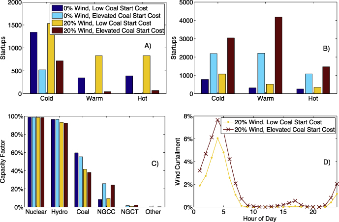
Figure 3. (A) Annual coal startups across the four scenarios. (B) Annual flexible-unit startups. (C) Average capacity factor by unit type. NGCC and NGCT indicate natural gas combined and simple cycle units, respectively. (D) Hourly average wind curtailment versus hour of day, as a percentage of average available wind in that hour, for 20% wind scenario with low and elevated coal start costs. Total wind curtailment in the low start cost and elevated start cost scenarios were 1.1% and 1.8%, respectively.
Download figure:
Standard image High-resolution imageThe scenarios in which elevated coal startup costs were incorporated showed dramatic reductions in coal startups over the low coal start cost scenarios. As expected, flexible units appear to have compensated and startups for these units increased dramatically over the low coal startup cost scenarios. As shown in figure 3(C), coal capacity factors were reduced under the high wind and elevated coal startup cost scenarios. Capacity factors for natural gas simple and combined cycle units increased slightly with wind penetration and more substantially with elevated coal startup costs. Figure 3(D) shows that incorporating elevated coal startup costs had the effect of increasing curtailment of wind up to nearly 2% of available wind energy, most of it occurring in the early morning hours.
Table 3 shows emissions from normal operations, as well as startup-related emissions of CO2, SO2, and NOX, which increased by approximately a factor of 2 under the 20% wind scenario. However, startups represented a small portion of overall emissions: a maximum of 2% across all scenarios. Incorporating elevated coal startup costs had the effect of substantially reducing startup-induced emissions, but, more significantly, also reduced emissions during normal operations. This is due to increased utilization of gas units as opposed to coal units.
Table 3. Annual emissions of CO2, NOX, and SO2 across the three scenarios.
| 0% wind, low coal start cost | 0% wind, elevated coal start cost | 20% wind, low coal start cost | 20% wind, elevated coal start cost | ||
|---|---|---|---|---|---|
| Normal operations | CO2 (Mton) | 210 | 200 | 150 | 140 |
| NOX (Mlb) | 740 | 690 | 470 | 420 | |
| SO2 (Mlb) | 4500 | 4200 | 3100 | 2800 | |
| Startups | CO2 (Mton) | 1.0 | 0.63 | 2.0 | 0.99 |
| NOX (Mlb) | 4.3 | 2.1 | 9.5 | 3.5 | |
| SO2 (Mlb) | 18 | 9.1 | 42 | 15 |
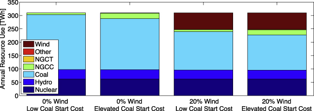
Resource use varied substantially across the three scenarios considered and is shown in figure 4. Comparing the first and third columns shows that the addition of 20% wind largely had the effect of displacing energy production by coal units, leaving nuclear and hydro production virtually unchanged. The scenario incorporating elevated startup costs for coal units had the effect of further displacing coal and replacing it by combined cycle gas.
Figure 4. Annual resource use in PJM West across the three scenarios. NGCT and NGCC indicate simple and combined cycle natural gas, respectively.
Download figure:
Standard image High-resolution image
Table 4 shows a range of economic indicators across the four scenarios, for suppliers as a whole, and for coal units in particular. Producer surpluses, and changes in consumer surplus over the 0% wind/low coal start cost scenario, were calculated. Producer surplus here includes the difference between annual revenues and total production costs, and consumer surplus is the area between the demand curve and the market-clearing price in each period, summed over the year. Note that since we have modeled demand as inelastic, we set a price cap and report only differences in consumer surplus. Revenue and surplus figures were calculated using prices generated endogenously in the UCED model. These prices do not account for congestion or transmission costs and we include them simply to illustrate that startup costs can make an important contribution to energy prices.
Table 4. Normal operations and start costs, revenues and profits for all unit types (including coal) and coal in three scenarios. Normal operations costs include fuel and variable O&M. Total production costs are the sum of normal operations and startup costs.
| 0% wind, low coal start cost | 0% wind, elevated coal start cost | 20% wind, low coal start cost | 20% wind, elevated coal start cost | |||||
|---|---|---|---|---|---|---|---|---|
| All | Coal | All | Coal | All | Coal | All | Coal | |
| Normal operations cost ($B) | 5.7 | 5.2 | 5.9 | 4.8 | 4.2 | 3.6 | 4.3 | 3.2 |
| Total startup costs | 0.29 | 0.27 | 0.18 | 0.12 | 0.53 | 0.50 | 0.27 | 0.19 |
| PJM start cost ($B) | 0.060 | 0.042 | 0.071 | 0.018 | 0.11 | 0.082 | 0.11 | 0.029 |
| Startup costs not included in PJM bids ($B) | 0.23 | 0.23 | 0.11 | 0.10 | 0.42 | 0.42 | 0.16 | 0.16 |
| Total production costs ($B) | 5.99 | 5.47 | 6.08 | 4.92 | 4.73 | 4.1 | 4.57 | 3.39 |
| Producer revenues ($B) | 8.8 | 5.9 | 9.8 | 6.1 | 6.4 | 3.8 | 7.3 | 4.0 |
| Producer surplus ($B) | 2.8 | 0.43 | 3.7 | 1.2 | 1.7 | −0.30 | 2.7 | 0.61 |
| Consumer surplus change over 0% wind, low coal start cost scenario ($B) | — | — | −1.0 | −1.0 | 1.1 | 1.1 | 0.12 | 0.12 |
Under business as usual coal startup costs, the wind-induced increase in startups was associated with an 80% increase in total startup costs. The majority of this increase was borne by coal units. Incorporating elevated coal startup costs reduced coal cycling costs dramatically and though it is clear from figure 3(C) that coal capacity factors were reduced in this scenario, the impact on coal unit surpluses was less clear. Table 4 shows that, on the aggregate, producer surpluses were −$300M for coal plants in the high wind/low start cost scenario. However, when elevated coal startup costs were incorporated, aggregate coal unit producer surpluses increased to $610M due partially to a reduction in cycling and partially to a 12% increase in average energy prices over the high wind/low start cost scenario. We again emphasize the limited ability of our modeling framework to forecast prices.
4. Conclusions
A study was conducted for the PJM West area to determine the effect of wind on the cycling of coal-fired power plants, emissions of CO2, NOX, and SO2, and production costs. High wind penetration scenarios were examined both under business as usual coal startup cost bidding, and under elevated coal startup cost bidding. When only the business as usual coal startup costs were used in the optimization, results indicated that wind penetration increased cycling of slow-ramping coal units and that this cycling led to emissions and cost penalties for these plants. On a system level, the magnitude of the penalties was found to be small compared to the overall savings associated with wind. By incorporating the full costs of coal cycling in the dispatch model, emissions and cost penalties associated with cycling were reduced. This scenario is representative of the decision of coal operators to change their bidding strategies to reflect full startup costs. Including full startup costs reduced coal capacity factors due to switching from coal to gas. However, the increase in energy prices associated with this switching led to increased surplus for coal plants compared to the high wind/business as usual startup cost scenario.
Our result that coal producer surpluses increased when elevated coal startup costs were incorporated deserves further discussion. Predictions of energy prices are inherently uncertain. This means that the result should be viewed with some caution. Also, while we have argued that bidding elevated startup costs would increase producer surpluses for coal operators in the high wind scenario, it is not certain that such bidding would occur. Since operators are trying to maximize overall profits, it may be more optimal to under-bid startup costs so as to earn higher revenues in the energy market. Under the increased startup requirements of a high wind scenario, we consider it likely, but not certain, that such a strategy would be less viable. Our high wind, high coal startup cost scenario should therefore be considered as a bounding case, and interpreted with the uncertainty in bidding strategies in mind.
Our modeling framework made a number of assumptions and approximations. While we do not expect the lack of transmission constraints to affect the implications of the aggregate results, it could affect the individual generators called on to perform cycling. Though we have focused on shutdown–startup cycles because of their larger per unit costs, it remains unclear whether changes in load cycling, in which output is increased or decreased without shutting down, could be a major cost driver. Also, while we have focused here on the current fleet of plants, several policy and economic factors may lead to a change in the composition of the fleet in the coming years. Finally, our analysis was based on the PJM West region. While we expect many of our qualitative results to hold for systems with different fuel mixes, care must be taken in generalizing our results to these other systems. In future work, we expect to examine some of these issues in more detail.
Despite the aforementioned limitations, we expect our qualitative conclusions regarding coal cycling are robust. Incorporating full cycling costs in bids transfers the burden of balancing wind to units that can perform this service at lower cost, has environmental benefits and could improve the profitability of coal plants in a high wind scenario. Incorporating full startup costs into unit commitment may be a good strategy for reducing the burden of coal cycling in a high wind future.
Acknowledgments
This work was conducted with the support of CMU's RenewElec Project and as part of the National Energy Technology Laboratory's Regional University Alliance (NETL-RUA), a collaborative initiative of the NETL, under the RES contract DE-FE0004000. The results and conclusion of this paper are the sole responsibility of the authors and do not the represent the views of the funding sources. We would like to thank Bri Matthias Hodge, Jay Apt, Roger Lueken, Allison Weis, and Todd Ryan for helpful comments and discussions.
Footnotes
- 1
In keeping with current operations of electric power systems, emissions are not included in the objective function constrained in the UCED.